Model-consistent estimation of the basic reproduction number from the incidence of an emerging infection

Abstract

We investigate the merit of deriving an estimate of the basic reproduction number early in an outbreak of an (emerging) infection from estimates of the incidence and generation interval only. We compare such estimates of with estimates incorporating additional model assumptions, and determine the circumstances under which the different estimates are consistent. We show that one has to be careful when using observed exponential growth rates to derive an estimate of , and we quantify the discrepancies that arise.

1 Introduction

The basic reproduction number R ₀ of an infectious agent is defined as the expected number of secondary cases caused by one typical infected individual in a population consisting of susceptibles only [3,6,7]. When an outbreak has started and the approximation that the population is fully susceptible no longer holds, one generally refers to the effective reproduction number R. The value of R ₀ is, as a rule, different for different infectious agents and depends among other things on the characteristics of the population that the agent invades. Given this, it is not immediate that one can adopt previously determined values or size ranges for a new outbreak, unless many of the complicated characteristics of, for example, population composition and contact structure are comparable. For various reasons one can be interested in the value of R ₀ or R early in an outbreak and during the outbreak. Notably, under a homogeneous mixing assumption, the values give insight into the extent of the control problem and a means of calculating how much control effort is needed.

In recent years several new methods for estimating R ₀ from outbreak data have been published, either as a general tool or for specific applications [4,9,11,17,21,24]. Some, like Wallinga and Teunis [24] do not need much data, but require knowledge of the generation time distribution. Most of these methods, however, are data-hungry: they either need contact information, use the whole outbreak time series (so are effectively retrospective measures), or increase in accuracy as the time series becomes longer. While several methods are promising many problems remain, and for various reasons. For example, we do not observe infections we observe detections, i.e. individuals (people, animals, farms, plants) exhibiting symptoms. There is then a possibly unknown incubation period distribution that convolutes the infection process into the observed process. Detections are not necessarily in the order of infection. Moreover, R ₀ is a generation-based concept [12], but generations are not observed—a daily number of new detections is observed from possibly mixed generations. Early in the outbreak stochastic influences play a large role. Also, heterogeneity between individual infectivity and susceptibility and in contact pattern may cause the distribution of which R ₀ is the mean to be highly skewed (e.g. [16]). To make matters worse, we almost never have data from an uncontrolled situation — some control measures, effective or not, often operate from the moment of detection of the index case.

Despite advances, but in light of the problems encountered, many publications in which R ₀ is estimated from outbreak data still depend on cumulative incidence and generation interval only (see for example [5,8,14,18,26]). As a rule, the cumulative incidence in outbreaks of an infectious disease is observed to initially grow approximately exponentially with time (and hence the incidence grows exponentially too). A frequently used approach is to fit an exponential function to the (cumulative) incidence and to use the approximate relationship to estimate R ₀, where r is the exponential growth rate and T _G is the observed mean generation interval of the epidemic. For rT _G small the further approximation is sometimes used. Many of the problems mentioned above apply to these estimates. For example, the ‘real’ value of r is not observed, not only because of control measures in operation but also due to the stochasticity in the early phase. In addition, the definition of the generation interval is not always consistently used and the method presupposes that the population is homogeneously mixing. Still, the method is easy and intuitive and one can wonder in which circumstances it would be a ‘good’ approximation, and how large discrepancies can be when these circumstances are not met. In this paper we investigate these questions.

2 Model-consistent estimation of R₀

We now derive estimates of R ₀ based on specific models and compare these with the previously mentioned approximations, which we denote and . We need to emphasise that R ₀ is independent of timescale, whereas T _G has dimension time and r has dimension time⁻¹. We also need to emphasise that we do not know r or T _G, we assume that they have been estimated from data in some way, for example by estimating the doubling time of the incidence, D, and writing r = log(2)/D. We do not write ^r or ^T _G for these estimates, as this would result in far too many hats in one paper.

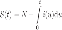
Assume for simplicity that the population is mixing homogeneously. The incidence of an emerging infection may be calculated from

where δ(t), a unit spike, is the incidence of infection at time zero, the kernel A(τ) is the expected infectivity of an infected as a function of τ, the time since exposure to infection [1,6,19]. The number in the population susceptible at time t is

For an emerging infection we assume the entire population to be susceptible at time zero. If this is not the case, we take N to be the size of the susceptible population prior to infection. As a first step towards developing a model, we specify the general form of the kernel A(τ). We write A(τ) = R ₀ f(τ), where R ₀ is the basic reproduction number that we wish to estimate, and f(τ) is the infectivity kernel, which is also the probability distribution of the generation interval.

For an emerging infection we have little information about f. We may have observations of the latent period (the time from exposure to infection to becoming infectious, T _E); the incubation period (the time from exposure to infection to the onset of symptoms) which we may in some cases assume to equal T _E; or the infectious period T _I. Given these we may wish to impose a particular form on the kernel, and use our limited knowledge to estimate parameter values for the distribution. These estimates may be revised as more information becomes available.

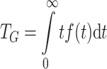
One quantity of interest is the mean generation interval of the epidemic, which is taken here to be the mean time from an individual’s exposure to infection to exposing others to infection (see [10], for an insightful exposition). We refer not to the time to the first occurrence of a secondary infection, but to the average time to all secondary infections. Alternatively, and equivalently, it can be defined as the expected duration of the primary infection at the time that a secondary infection occurs (see [22]). The mean generation interval may be determined from the formula

Given a probability distribution for the generation interval, f(τ), and an estimated initial rate of exponential increase for the epidemic, r, we approximate the initial stages of the epidemic by i(t) = e ^rt with S(t) ≃ N. Equation (1) then leads to a model-consistent estimate of the basic reproduction number via the formula

(see [6]). If f(t) were a delta function, then Eqs. (2, 3) would lead to the estimate R ₀ = R ⁺₀. For the SIR model, where f(t) = γe ^−γt, Eqs. (2, 3) lead to the estimate R ₀ = R ⁻₀. We now computeR ₀ for three distribution functions which may be used as kernels: those with a fixed, exponentially or trapezoidally distributed infectious period (see Fig. 1). We refer to these as R ^fix₀, R ^exp₀ and R ^trap₀, respectively. We also compute R ₀ for the model with latent and infectious periods that each have gamma distributions, referred to as R ^(m,n)₀. We have R ^exp₀ = R ^(1,1₀)} and R ^fix₀ = lim_m,n→∞ R ^(m,n)₀.

Fig. 1.

A selection of kernels, f(τ) that may be used to model emerging infections: kernels due to fixed and exponentially distributed latent and infectious periods are shown as dashed and dashed/dotted lines, respectively; and the trapezium kernel is shown as a solid line. All kernels are scaled to have integral one. a Kernels suitable for modelling influenza, with latent period T _E = 1.6 days and infectious period T _I = 4.0 days. b Kernels suitable for modelling SARS, with latent period T _E = 5.5 days and infectious period T _I = 7.0 days

2.1 Fixed infectious period

Given fixed latent and infectious periods, T _E and T _I respectively, and assuming f constant when non-zero, we have f(τ) = 1/T _I for T _E < τ < T _E+ T _I and f(τ) = 0 otherwise. For this distribution T _G = T _E + T _I/2 and

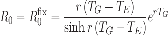R ⁺₀ is useful as an estimator for R ^fix₀ when the latent period may be regarded as fixed and the infectious period is short relative to the timescale 1/r (rT _I is small). As sinh x > x whenever x > 0, and 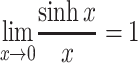we have R ^fix₀ ≤ R ⁺₀, and 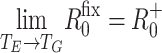. Wallinga and Lipsitch [23] showed that R ⁺₀ is an upper bound on estimates of R ₀ for any distribution f(t).

2.2 Trapezoidal infection kernel

Consider the kernel

This is a suitable approximation to an infectivity function where nobody is infectious before τ _a time units or after τ _d time units post-exposure, maximum infectivity occurs between τ _b and τ _c time units after exposure, and contact rates are constant. The distribution is consistent with a mean latent period of , a mean infectious period of and a mean generation interval of 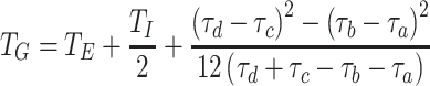Hence, if the trapezium is symmetric , which is the same relationship as that for the fixed infectious period. The basic reproduction number solves R ^trap₀ ¯f(r) = 1, where ¯f(s) is the Laplace transform of f(t) (see Appendix 1)

2.3 SEIR differential equation models

In an extended SEIR differential equation model the population of size N is made up of S susceptibles, E that have been exposed to infection but are not yet infectious, I infectious and R that have been infected and recovered. If the epidemic processes have a much faster timescale than the demographic processes, we obtain the equations

The exposed and infectious classes have been subdivided E = Σ^m_i=1 E _i and I = Σⁿ_j=1 I _j, respectively. The times spent in the exposed and infectious classes are gamma distributed with means T _E = 1/ν and T _I = 1/γ, respectively, andR ₀ = β/γ. The mean generation interval is (see Appendix 2). If the initial rate of exponential increase of the epidemic is r, then

This result is derived in Appendix 2, where it is also shown that given values of r, T _E and T _G, R ^(m,n)₀ is an increasing function of both m and n.

2.4 Exponentially distributed infectious period

The well-known SEIR differential equation model is the special case of Eqs. (6) with m = n = 1. For this model the times spent in the exposed and infectious classes are exponentially distributed with means T _E = 1/ν and T _I = 1/γ respectively, and the appropriate kernel function in Eqs. (2, and 3) is (see [6]). The mean generation interval is , and given r we have

The approximation is appropriate for the SIR model, for which ν → ∞, T _E → 0 and T _G → T _I = 1/γ. Hence R ⁻₀ performs best as an estimate when either the latent period T _E or the infectious period T _I is small compared to T _G, and performs worst when they are equal.

3 Method and results

We assumed that we had estimated values of the initial rate of exponential increase of infection incidence, r, the mean latent period, T _E, and the mean generation interval, T _G. We then used Eqs. (4, and 7) to calculate model-based estimates of the basic reproduction number using the assumptions of a fixed or exponentially distributed infectious period, leading to R ^fix₀ and R ^exp₀, respectively. We did this for values of the ratio of the latent period to the generation interval, T _E/T _G, in the range zero to 0.99. The values of R ^fix₀ and R ^exp₀ are plotted as functions of T _E/T _G for rT _G = 0.5, 1.0, 1.5, 2.0 in Fig. 2, and compared with the values of the estimators and in those cases. When rT _G = 0.5, 1.0, 1.5 or 2.0 we have R ⁻₀ = 1.5, 2.0, 2.5 or 3.0 and R ⁺₀ = 1.65, 2.72, 4.48 or 7.39, respectively.

Fig. 2.

Estimates of the basic reproduction number R ₀ as a function of the ratio of the latent period to the mean generation interval, T _E/T _G. The solid plots are a,b fixed infectious period: R ^fix₀ with rT _G = 0.5 (lower), rT _G = 1.5 (upper); and rT _G = 1.0 (lower), rT _G = 2.0 (upper) respectively, and c,d exponentially distributed infectious period: R ^exp₀ with rT _G = 0.5 (lower), rT _G = 1.5 (upper); and rT _G = 1.0 (lower), rT _G = 2.0 (upper), respectively. The horizontal dotted and dashed lines indicate the corresponding values of and , respectively

The results shown in Fig. 2 illustrate that for fixed values of r, T _E and T _G, the values of R ⁻₀ and R ⁺₀ are lower and upper bounds, respectively for both R ^exp₀ and R ^fix₀. In Sects. (2.1 and 2.4) it was shown that R ^fix₀ ≤ R ⁺₀ and R ⁻₀ ≤ R ^exp₀, respectively. It is proved in Appendix 2 that R ^(m,n)₀ 0 is an increasing function of both m and n. Putting these results together we obtain the inequality

where m and n are any finite positive integers.

Table 1 was constructed to illustrate the results that may be obtained for some specific infections. Parameters were chosen from the literature to be representative of influenza [20], severe acute respiratory syndrome (SARS) [19], smallpox [1] and foot and mouth disease (FMD) [11]. For each infection a trapezium distribution was constructed for f(τ), and used together with an estimate of R ₀ to calculate an estimate of the initial exponential increase, r. The function f(τ) was also used to calculate values for the mean generation interval T _G, the mean latent period T _E and the mean infectious period T _I.

Table 1.

Estimates of R ₀ that could be made for emerging infections

Infection	r	T G	T E	T I	R −0	R +0	R fix0	R exp0	R trap0
Influenza	0.198	3.65	1.60	4.10	1.72	2.06	2.00	1.85	2.00
SARS	0.134	9.00	5.50	7.00	2.21	3.34	3.22	2.55	3.20
Smallpox	0.0576	20.5	15.0	11.0	2.18	3.26	3.20	2.45	3.20
FMD	0.165	6.00	2.00	8.00	1.99	2.70	2.51	2.21	2.50

The initial rate of exponential increase (r day⁻¹), mean generation interval (T _G days), mean latent period (T _E days) and mean infectious period (T _I days) that could be observed for epidemics of influenza, SARS, smallpox; and for foot andmouth disease (FMD) spreading between farms; together with the corresponding estimates of the basic reproduction numbermade using the approximations R ⁻₀ = 1+rT _G and , or assuming a rectangular, exponential or trapeziodal distribution for the infectious period, leading to R ^fix₀ R ^exp₀ and R ^trap₀, respectively

If these values of r, T _G and T _E had been estimated from data, and then R ₀ had been estimated by R ⁻₀, R ⁺₀, R ^fix₀, R ^exp₀ or R ^trap₀, the estimates presented in Table 1 would have resulted. By construction, the estimated value of R ^trap₀ then corresponds to the assumed value of R ₀. Hence Table 1 must be regarded as a comparison of estimates that may be made; the relative values are important rather than the absolute values.

4 Conclusions and discussion

We have derived and discussed model-consistent methods for estimating the basic reproduction number (R ₀) for an infectious disease from the initial rate of exponential growth of incidence of infection (r) at the beginning of an epidemic. These methods can only be applied to incidence data from the period where it is reasonable to assume that the whole population may be regarded as susceptible (S(t) }~ N).

Among the first pieces of information obtained for an emerging infection are observations of the latent and infectious periods. These may be used as estimates to construct a rectangular kernel for an integral equation model, or to derive rate parameters for a differential equation model. Examples of infectivity kernels with the same latent and infectious periods are shown in Fig. 1. These kernels appear to be quite different, with the exponential kernel allowing some transmission of infection from time zero, and exhibiting a long infection tail. These features can lead to disparities in the results from modelling exercises. The transmission at early times mitigates against the success of control methods based on contact tracing, or any other method with inherent delays. The tail can lead to transmission appearing to continue in the model long after control measures should have eliminated the infection. The trapezoidal kernels also shown in Fig. 1 allow for some variability in the fixed and latent periods to be incorporated in the model. For example, the kernel shown as suitable for modelling influenza (Fig. 1a) is consistent with a latent period uniformly distributed between 1.2 and 2.0 days, and an infectious period of 4.0 days. The kernel shown as suitable for modelling SARS (Fig. 1b) is consistent with nobody being infectious before 4 days, everybody infectious by 7 days, everybody still infectious at 11 days and nobody infectious after 14 days; with the proportion infectious at intermediate times determined by linear interpolation. As well as allowing for some variability, the trapezoidal kernel has the advantage over the rectangular one that it is a continuous function, and this avoids problems with numerical schemes that do not allow discontinuities. Of course, if further information is available, then other distributions may be more appropriate.

Figure 2 compares estimates of the basic reproduction number based on fixed (Fig. 2a, 2b) and exponentially distributed (Fig. 2c, 2d) infectious periods, R ^fix₀ andR ^exp₀, respectively, with the estimates based only on mean generation interval, and . The estimate R ⁻₀ is inaccurate whenever rT _G is not small. Using the fixed infectious period model, R ⁺₀ approximates R ^fix₀ when T _E/T _G is near to one, that is when the infection has a long latent period and a short infectious period. The estimate R ⁻₀ is an approximation to R ^exp₀ if either the latent period or infectious period are very short, but R ⁺₀ is never a good estimator for R ^exp₀ and it’s use is therefore inconsistent with an SEIR model.

The estimates of R ₀ derived in this paper have the ordering R ⁻₀ ≤ R ^exp₀ ≤ R ^(m,n)₀ < R ^fix₀ ≤ R ⁺₀. This inequality establishes that, given the same values of r, T _E and T _I, R ⁻₀ provides a closer estimate for R ^exp₀ than for R ^fix₀, and R ⁺₀ provides a closer estimate for R ^fix₀ than for R ^exp₀. Even though results derived from the gamma distributed kernel, R ^(m,n)₀, are not displayed in Fig. 2, we have established that R ^fix₀ and R ^exp₀ are upper and lower bounds respectively for R ^(m,n)₀. Note that for the model with a fixed infectious period, , but for the model with an exponentially distributed infectious period, . The inequality, and the results presented in Fig. 2 are derived on the assumption that T _E and T _G are the same in both models; T _I is defined consistently with the model, and hence differs between models. This is in contrast to the distributions presented in Fig. 1, which have the same latent and infectious periods, T _E and T _I, and hence different mean generation intervals T _G.

Table 1 shows results that could be obtained when estimating R ₀ for emerging infections, with parameters suitable for these infections. The parameter values indicated for each infection should be regarded as sensible values rather than exact estimates, and the results are presented to indicate the relevance of Fig. 2. For all four examples there is close agreement between R ^fix₀ and R ^trap₀. This is not surprising for the influenza example where the trapezium kernel has steep sides (Fig. 1a), but also applies for examples such as SARS (Fig. 1b). The results in Table 1 confirm that if rT _G is small, hence R ⁻₀ is close to one, then R ⁻₀ may be used as an estimator for R ^exp₀ when an exponential model is appropriate. If a model with a fixed infectious period is more appropriate then R ⁺₀ is a better estimate for R ^fix₀, especially when T _E /T _G is closer to one: compare for example the relative values of R ⁺₀ and R ^fix₀ for smallpox where T _E /T _G = 0.73 and FMD where T _E /T _G = 0.33.

Recently other estimation methods have been suggested as improvements on R ⁻₀ and R ⁺₀. Wearing et al. [25] compared estimates based on R ^exp₀ with results obtained using gamma-distributed infection kernels. Lloyd [15] found similar results for models of within-host virus dynamics. Heffernan and Wahl [13] also examined the problem, and provided correction factors for estimates of R ₀ based on both the mean and variance of observed transition times. Wallinga and Lipsitch [23] used a similar approach to ours, and derived estimates of R ₀ for a selection of infectivity kernels f(t), including those derived from a gamma-distributed infectious period but only with T _E = 0. They also considered the case where f(t) is a Normal distribution; if employed though this distribution should be truncated to avoid the possibility of negative generation intervals.

Even though we selected a number of particular kernels for our study, and these cover a reasonable range of first choices, our method is applicable to all biologically sensible kernels. When estimating kernels from data, one should be careful. Estimates made early in an epidemic are likely to be based on household studies, and may be truncated due to local saturation of contacts. In addition, it is unclear how valid such estimates are when extrapolated to the wider community with multiple levels of mixing.

We must be careful in attempting to draw conclusions from our analysis. As a new infection emerges the appropriate model is speculative, and in any situation there is no such thing as the correct model. For example, in the context of pandemic influenza, Ferguson et al. [8] had T _G = 2.6 and T _E = 1.48 days, and estimated R ₀ ≈ R ⁻₀, obtaining values in the range 1 – 2. Their model was more complex than those discussed here, but we have seen that for low values of rT _G, R ⁻₀ provides a reasonable estimate. Mills et al. [18] used an SEIR model, and estimated R from R ^exp₀ which is consistent with their model. Our approach is to advocate using an estimate of R ₀ that is consistent with the model used to evaluate control strategies.

Appendix 1: The derivation of R^trap₀

To find the Laplace transform of the trapezoidal distribution (5), define the functions

and

Then, given an estimated value of r, the basic reproduction number solves

Appendix 2: The proof of inequality (8)

For the extended SEIR model (6)the probability that an individual infected at time zero is in one of the infected classes (E _i or I _j) at time t is found by solving the differential equations with β = 0, E ₁(0) = 1, E _i(0) = 0 for i = 2,…, m and I _j(0) = 0 for j = 1,…, n. In the Laplace transform domain the solutions are

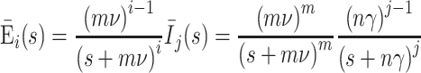The probability that an individual infected at time zero has become infectious or has ceased to be infectious by time t is h(t) or g(t) respectively, where

Back-transforming,

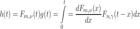where

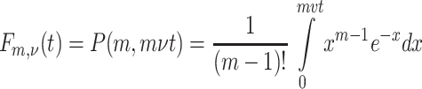is a regularized incomplete gamma function (see 6.5.1, [2]). The infectivity kernel has Laplace transform

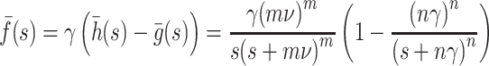The generation interval is given by the formula

If the initial rate of exponential increase of the epidemic is r, then R ^(m,n)₀ ¯f(r) = 1, hence

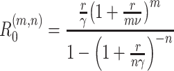This result may be found in Wearing et al. [25]. The function (1 + x/m)^m is positive for positive x, and increases monotonically from 1 + x to e ^x as m increases from 1 to ∞. Hence, given values of r, ν and γ, R ^(m,n)₀ is an increasing function of m, but a decreasing function of n. However, substituting and 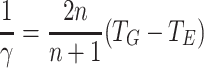we obtain

The function

is positive for positive x, and increases monotonically from 1+ x/2 to as n increases from 1 to ∞. The proof is a straightforward but tedious manipulation of expressions: we multiply the numerator and denominator of the expression for f _n(x) by (1+x/(n+1))ⁿ and then show that for n≥ 1 and x > 0. Hence, given values of r, T _E and T _G, R ^(m,n)₀ is an increasing function of both m and n. In the limit as m and n tend to infinity, R ^(m,n)₀ tends to R ^fix₀. Hence for all positive finite integers m and n, , completing the proof of inequality (8).

References

- 1.Aldis G.K., Roberts M.G. An integral equation model for the control of a smallpox outbreak. Math. Biosci. 2005;195:1–22. doi: 10.1016/j.mbs.2005.01.006. [DOI] [PubMed] [Google Scholar]
- 2.Abramowitz M., Stegun I.A. Handbook of Mathematical Functions. New York: Dover; 1964. [Google Scholar]
- 3.Anderson R.M., May R.M. Infectious Diseases of Humans: Dynamics and Control. New York: Oxford Press; 1991. [Google Scholar]
- 4.Cauchemez S., Boële P.-Y., Donnelly C.L., Ferguson N.M., Thomas G., Lueng G.M., Hedley A.J., Anderson R.M., Valeron A.-J. Real-time estimates in early detection of SARS. Emerg. Infect. Dis. 2006;12:110–113. doi: 10.3201/eid1201.050593. [DOI] [PMC free article] [PubMed] [Google Scholar]
- 5.Choi B.C.K., Pak A.W.P. A simple approximate mathematical model to predict the number of severe acute respiratory syndrome cases and deaths. J. Epidemiol. Commun. Health. 2003;57:831–835. doi: 10.1136/jech.57.10.831. [DOI] [PMC free article] [PubMed] [Google Scholar]
- 6.Diekmann O., Heesterbeek J.A.P. Mathematical Epidemiology of Infectious Diseases: Model Analysis and Interpretation. New York: Wiley; 2000. [Google Scholar]
- 7.Diekmann O., Heesterbeek J.A.P., Metz J.A.J. On the definition and computation of the basic reproduction ratio R0 in models for infectious diseases in heterogeneous populations. J. Math. Biol. 1990;28:365–382. doi: 10.1007/BF00178324. [DOI] [PubMed] [Google Scholar]
- 8.Ferguson N., Cummings D.A.T., Cauchemez S., Fraser C., Riley S., Meeyai A., Iamsirithaworn S., Burke D.S. Strategies for containing an emerging influenza pandemic in Southeast Asia. Nature. 2005;437:209–214. doi: 10.1038/nature04017. [DOI] [PubMed] [Google Scholar]
-
9.Ferrari M.J., Bjørnstad O.N., Dobson A.P. Estimation and inference of
of an infectious pathogen by a removal method. Math. Biosci. 2005;198:14–26. doi: 10.1016/j.mbs.2005.08.002. [DOI] [PubMed] [Google Scholar]
- 10.Fine P.E.M. The interval between successive cases of an infectious disease. Am. J. Epidemiol. 2003;158:1039–1047. doi: 10.1093/aje/kwg251. [DOI] [PubMed] [Google Scholar]
- 11.Haydon D., Chase-Topping M., Shaw D.J., Matthews L., Friar J., Wilesmith J., Woolhouse M.E.J. The construction and analysis of epidemic trees with reference to the 2001 UK foot-and-mouth outbreak. Proc. R. Soc. Lond B. 2003;270:121–127. doi: 10.1098/rspb.2002.2191. [DOI] [PMC free article] [PubMed] [Google Scholar]
12.Heesterbeek J.A.P. A brief history of
and a recipe for its calculation. Acta. Biotheor. 2002;50:189–204. doi: 10.1023/A:1016599411804. [DOI] [PubMed] [Google Scholar]
- 13.Heffernan J.M., Wahl L.M. Improving Estimates of the basic reproductive ratio: using both the mean and dispersal of transition times. Theor. Popul. Biol. 2006;70:135–145. doi: 10.1016/j.tpb.2006.03.003. [DOI] [PMC free article] [PubMed] [Google Scholar]
- 14.Lipsitch M., Cohen E., Cooper B., Robins J.M., Ma S., James L., Gopalakrishna G., Chew S.K., Tan C., Samore M.H., Fisman D., Murray M. Transmission dynamics and control of severe acute respiratory syndrome. Science. 2003;300:1966–1970. doi: 10.1126/science.1086616. [DOI] [PMC free article] [PubMed] [Google Scholar]
- 15.Lloyd A.L. The dependence of viral parameter estimates on the assumed viral life cycle: limitations of studies of viral load data. Proc. R. Soc. B. 2001;268:847–854. doi: 10.1098/rspb.2000.1572. [DOI] [PMC free article] [PubMed] [Google Scholar]
- 16.Lloyd-Smith J.O., Schreiber S.J., Kopp P.E., Getz W.M. Superspreading and the effects of individual variation on disease emergence. Nature. 2005;438:355–359. doi: 10.1038/nature04153. [DOI] [PMC free article] [PubMed] [Google Scholar]
- 17.Meester R., de Koning J., de Jong M.C.M., Diekmann O. Modeling and real-time prediction of classical swine fever epidemics. Biometrics. 2002;58:178–184. doi: 10.1111/j.0006-341X.2002.00178.x. [DOI] [PubMed] [Google Scholar]
- 18.Mills C.E., Robins J.M., Lipsitch M. Transmissibility of 1918 pandemic influenza. Nature. 2004;432:904–906. doi: 10.1038/nature03063. [DOI] [PMC free article] [PubMed] [Google Scholar]
- 19.Roberts M.G. Modelling strategies for minimizing the impact of an imported exotic infection. Proc. R. Soc. B. 2004;271:2411–2415. doi: 10.1098/rspb.2004.2865. [DOI] [PMC free article] [PubMed] [Google Scholar]
- 20.Roberts M.G., Baker M., Jennings L.C., Sertsou G., Wilson N. A model for the spread and control of pandemic influenza in an isolated geographical region. J. R. Soc. Interface. 2007;4:325–330. doi: 10.1098/rsif.2006.0176. [DOI] [PMC free article] [PubMed] [Google Scholar]
- 21.Stegeman J.A., Elbers A.R.W., Smak J., de Jong M.C.M. Quantification of the transmission of classical swine fever virus between herds during the 1997–998 epidemic in the Netherlands. Prevent. Veterinary Med. 1999;42:219–234. doi: 10.1016/S0167-5877(99)00077-X. [DOI] [PubMed] [Google Scholar]
- 22.Svensson A. A note on generation intervals in epidemic models. Math. Biosci. 2007;208:300–311. doi: 10.1016/j.mbs.2006.10.010. [DOI] [PubMed] [Google Scholar]
- 23.Wallinga J., Lipsitch M. How generation intervals shape the relationship between growth rates and reproductive numbers. Proc. R. Soc. Ser. B. 2007;274:599–604. doi: 10.1098/rspb.2006.3754. [DOI] [PMC free article] [PubMed] [Google Scholar]
- 24.Wallinga J., Teunis P. Different epidemic curves for severe acute respiratory syndrome reveal similar impacts of control measures. Am. J. Epidemiol. 2004;160:509–516. doi: 10.1093/aje/kwh255. [DOI] [PMC free article] [PubMed] [Google Scholar]
- 25.Wearing H.J., Rohani P., Keeling M.J. Appropriate models for the management of infectious diseases. PLoS Med. 2005;7:621–627. doi: 10.1371/journal.pmed.0020174. [DOI] [PMC free article] [PubMed] [Google Scholar]
- 26.Zhou G., Yan G. Severe acute respiratory syndrome epidemic in Asia. Emerg. Infect. Dis. 2003;9:1608–1610. doi: 10.3201/eid0912.030382. [DOI] [PMC free article] [PubMed] [Google Scholar]