A new multi-neuron spike-train metric

Abstract

The Victor-Purpura spike-train metric has recently been extended to a family of multi-neuron metrics and used to analyze spike trains recorded simultaneously from pairs of proximate neurons. The Victor-Purpura metric is one of the two metrics commonly used for quantifying the distance between two spike trains, the other is the van Rossum metric. Here, we suggest an extension of the van Rossum metric to a multi-neuron metric. We believe this gives a metric which is both natural and easy to calculate. Both types of multi-neuron metric are applied to simulated data and are compared.

1 Introduction

A key current challenge is understanding how neurons in the primary sensory regions encode their input stimuli. One technique is to use a spike-train metric to cluster the responses to a set of stimuli. By assessing how successfully the clusters match the stimuli it is possible to tell how successfully a given metric utilizes the most salient features in a neuronal response.

This technique is used, for example, in (Narayan et al., 2006) as a tool to investigate the response of songbird neurons to songs. In the experiment, recordings are made of the neuronal responses of field L neurons of the anesthetized Zebra Finch to 10 repetitions each of 20 con-specific songs. The van Rossum metric (van Rossum, 2001) is then used to work out the distance between pairs of spike trains and a simplified k-means type clustering algorithm is used to divide the 200 spike trains into 20 clusters.

To calculate the van Rossum metric the spike train is first filtered to form a function: the spike train, considered as a list of spike times t = (t₁, t₂, · · · , t_n) is mapped to a real function using a kernel h(t):

$$\begin{array}{cc}\hfill & \mathcal{F}:\text{spike trains}\to \text{real functions}\hfill \\ \hfill \mathbf{t}& =(t_1,t_2,\dots ,t_n)\mapsto \mathcal{F}\left(\mathbf{t}\right)=\sum _{i=1}^{n}h(t-t_i).\hfill \end{array}$$ (1)

The distance between two spike trains, t₁ and t₂, is taken to be the distance between the two corresponding functions, using, for example, the standard L² metric on the space of real functions:

$$d_2({\mathbf{t}}_1,{\mathbf{t}}_2;h)=\sqrt{\int dt{(f_1-f_2)}^2}$$ (2)

where $f_1\left(t\right)=\mathcal{F}\left({\mathbf{t}}_1\right)$ and $f_2\left(t\right)=\mathcal{F}\left({\mathbf{t}}_2\right)$.

One common choice of kernel is the decaying exponential

$$h\left(t\right)=\{\begin{array}{cc}0\hfill & t<0\hfill \\ \frac{1}{\tau }{e}^{-t∕\tau }\hfill & t\ge 0\hfill \end{array}\phantom{\}}.$$ (3)

In (Narayan et al., 2006), this kernel is used with different values of the time constant τ. Different τ values give different metrics and different clusters. By calculating which clustering most accurately groups the spike trains by song stimulus, it is found that the best metric corresponds to τ ≈ 12 ms. This, it is argued, gives an indication of the timescales involved in neuronal responses in this part of the Zebra finch brain.

Another useful metric was introduced in (Victor and Purpura, 1996; Victor and Purpura, 1997). The Victor-Purpura distance between two spike trains is calculated by considering how one spike train could be transformed into the other using a sequence of small moves: deleting or adding a spike or moving a spike to another location. A cost of one is associated with adding or deleting a spike and a cost of q|δt| is associated with moving a spike by a time interval δt. The Victor-Purpura distance is then the cost of transforming one spike train into the other in the cheapest possible way.

The q parameter determines the cost of moving a spike. For q = 0 there is no cost and the Victor-Purpura distance between two spike trains is just the difference in the number of spikes. For q very large, in contrast, it is cheaper to delete and create spikes than to move a spike from one location to another and so the distance between two spike trains is the total number of non-coincident spikes. Roughly speaking, 2/q gives the time-difference interval for which two spikes can be considered to be related by jitter.

It should be determined experimentally whether the Victor-Purpura or the van Rossum is the more suitable spike-train metric. One nice feature of the Victor-Purpura metric is that it allows unreliability and jitter to be distinguished in the spiking response to repeated presentations of the same stimuli. On the other hand, the metric explicitly pairs spikes in the two spike trains; it is not clear whether this is a good property for a spike-train metric to have.

Because it involves a kernel function and a choice of metric on the function space, the van Rossum metric is very flexible. In fact, numerically, the Victor-Purpura distance is very similar to an L¹ van Rossum distance:

$$d_1({\mathbf{t}}_1,{\mathbf{t}}_2;h={\delta }_{2∕q})=\int dt\mid f_1-f_2\mid$$ (4)

where the kernel δ_2/q(t) is the block function

$${\delta }_{2∕q}\left(t\right)=\{\begin{array}{cc}q∕2\hfill & 0\le t<2∕q\hfill \\ 0\hfill & \text{otherwise}\hfill \end{array}\phantom{\}}$$ (5)

and q is the time-scale parameter in the Victor-Purpura metric. By considering simple cases, with small numbers of spikes, is easy to see why this might the case. We have checked that the two metrics are numerically similar for real data by computing the distance between 400 pairs of spike trains chosen at random from the collection of field L spike trains described in (Narayan et al., 2006). We have found that the average difference between the Victor-Purpura distance and van Rossum distance, with 2/q = 20 ms is 2.54% with a standard deviation of .08%.

It might be also interesting to consider a generalized Victor-Purpura metric which gains the flexibility of the van Rossum metric by changing the cost of moving a spike from q|δt| to f(|δt|) for some function f.

2 Multi-neuron metrics

It is pointed out in (Aronov et al., 2003) that it is useful to apply the clustering technique to simultaneous recordings from proximate neurons. This could help to uncover how populations of neurons cooperate to encode a sensory input. In order to cluster the response of, for example, a pair of neurons, a two-neuron metric must be defined. In (Aronov et al., 2003; Aronov, 2003) a family of multi-neuron metrics is defined; we will call these the ARMV metrics. In the ARMV metrics, spikes are labelled by the neuron that fired them, but this label can be changed at a cost of k, where k is a parameter. Hence, the ARMV distance between two sets of labelled spike trains is the cheapest set of small moves transforming one set into the other, where, now, the small moves are adding or deleting a spike at a cost of one, moving a spike by an interval δt at a cost of q|δt| and relabelling a spike at a cost of k.

In (Aronov et al., 2003) two different coding strategies for neuron populations are distinguished: a ‘summed population code’ (SP) metric where the two spike trains from the two neurons are super-imposed before the distance is calculated, and a ‘labeled line code’ (LL) metric where the distance is measured for each neuron separately and then added. These two possibilities correspond to the metrics at either end of the one-parameter family of ARMV metrics obtained by varying k. If k = 0 there is no cost to relabelling a spike and so this is a SP metric. On the other hand, if k ≥ 2 it costs more to relabel a spike than to delete a spike from one spike train and to add a spike in the other. Hence, for k ≥ 2 the ARMV distance between the two sets of spike trains is the same as the sum of the individual Victor-Purpura distances. Therefore, this is an SP metric.

To illustrate, the SP and LL two-neuron metric constructed from the van Rossum spike-train metric will be considered. Let t₁ and u₁ be the responses of the two neurons to the first stimulus presentation and t₂ and u₂ to the second and define the corresponding functions

$$\begin{array}{cc}\hfill & f_i\left(t\right)=\mathcal{F}\left({\mathbf{t}}_i\right)\hfill \\ \hfill & g_i\left(t\right)=\mathcal{F}\left({\mathbf{u}}_i\right)\hfill \end{array}$$ (6)

with i = 1, 2. Since a SP metric first superimposes the spike trains, the two-neuron SP distance between the responses to the two stimuli is given by

$$d_2[({\mathbf{t}}_1,{\mathbf{u}}_1),({\mathbf{t}}_2,{\mathbf{u}}_2);h,\mathrm{SP}]=\sqrt{\int dt{(f_1+g_1-f_2-g_2)}^2}$$ (7)

whereas the LL distance is the sum of the distances between stimuli for each neuron:

$$d_2[({\mathbf{t}}_1,{\mathbf{u}}_1),({\mathbf{t}}_2,{\mathbf{u}}_2);h,\mathrm{LL}]=\sqrt{\int dt{(f_1-f_2)}^2+\int dt{(g_1-g_2)}^2}$$ (8)

where, because this is an L² metric, the sum has been taken using the Theorem of Pythagoras. The purpose of this paper is to define a natural one-parameter family of metrics interpolating between these two possibilities. For simplicity, we will construct the two-neuron metrics in the next section, the multi-neuron metric is constructed in a similar way and is described in appendix 1.

3 The metrics

The idea behind the new metrics is to map the filtered spike trains f_a and g_a into the space of two-dimensional vector fields. The space of two-dimensional vector fields on the line

$$\{(f,g):f\left(t\right)\text{and}g\left(t\right)\text{are real functions}\}$$ (9)

can be thought of as the space of ordered pairs of functions. The space has an obvious norm whereby, the length is given by taking the usual Euclidean norm on the two-dimensional vector space and the L² norm on the function space:

$${\mid \mid (f,g)\mid \mid }_2=\sqrt{\int dt(f^2+g^2)}.$$ (10)

Now, if we associate each of the neurons with a two-dimensional unit vector, e, we can map its spike-trains into the space of two-dimensional vector fields

$$\begin{array}{cc}\hfill & {\mathcal{F}}_{\mathbf{e}}:\text{spike trains}\to \text{two}-\text{dimensional vector fields}\hfill \\ \hfill \mathbf{t}& =(t_1,t_2,\cdots ,t_n)\mapsto {\mathcal{F}}_{\mathbf{e}}\left[(t_1,t_2,\cdots ,t_n)\right]=\mathcal{F}\left(\mathbf{t}\right)\mathbf{e}=\left(\sum _{i=1}^{n}h(t-t_i)\right)\mathbf{e}.\hfill \end{array}$$ (11)

So, for example, if we assign the unit vector

$${\mathbf{e}}_0=\left(\begin{array}{c}\hfill 1\hfill \\ \hfill 0\hfill \end{array}\right)$$ (12)

to the first neuron then a spike train t = (t₁, t₂, · · · , t_n) from that neuron is mapped to the vector field

$${\mathcal{F}}_{{\mathbf{e}}_0}\left(\mathbf{t}\right)=\left(\begin{array}{c}\hfill \sum _{i=1}^{n}h(t-t_i)\hfill \\ \hfill 0\hfill \end{array}\right).$$ (13)

The two-neuron metric being proposed here is calculated by assigning different unit vectors to each of the two neurons. The metrics are parameterized by the angle between these vectors. It will be seen that varying this angle from zero to π/2 interpolates between the SP and LL metrics described above. For simplicity, the unit vector e₀ is assigned to the first neuron, and the vector

$${\mathbf{e}}_{\theta }=\left(\begin{array}{c}\hfill \cos \theta \hfill \\ \hfill \sin \theta \hfill \end{array}\right)$$ (14)

to the second. The total response vector field r is then formed by adding together the two vector fields associated with the two neurons. Hence, using the same notation as above, we have two response vector fields, one for each presentation

$$\begin{array}{cc}\hfill & {\mathbf{r}}_1=f_1{\mathbf{e}}_0+g_1{\mathbf{e}}_{\theta }\hfill \\ \hfill & {\mathbf{r}}_2=f_2{\mathbf{e}}_0+g_2{\mathbf{e}}_{\theta }.\hfill \end{array}$$ (15)

The distance between the two pairs of spike trains, (t₁, u₁) and (t₂, u₂), is defined as the distance between the two corresponding vector fields, given by the norm above:

$$d_2[({\mathbf{t}}_1,{\mathbf{u}}_1),({\mathbf{t}}_2,{\mathbf{u}}_2);h,\theta ]=\mid \mid {\mathbf{r}}_1-{\mathbf{r}}_2\mid {\mid }_2.$$ (16)

Expanding in terms of the f_a and g_a

$$\begin{array}{cc}\hfill d_2[({\mathbf{t}}_1,{\mathbf{u}}_1),({\mathbf{t}}_2,{\mathbf{u}}_2);h,\theta ]& =\sqrt{\int dt(\delta f^2+\delta g^2+2c\delta f\delta g)}\hfill \\ \hfill & =\sqrt{d_2{[({\mathbf{t}}_1,{\mathbf{u}}_2),({\mathbf{t}}_2,{\mathbf{u}}_2);h,\mathrm{LL}]}^2+2c\int dt\delta f\delta g}\hfill \end{array}$$ (17)

where δf = f₁ — f₂, δg = g₁ — g₂ and c = cosθ. It is clear from these formula that

$$d_2[({\mathbf{t}}_1,{\mathbf{u}}_1),({\mathbf{t}}_2,{\mathbf{u}}_2);h,\theta =0]=d_2[({\mathbf{t}}_1,{\mathbf{u}}_2),({\mathbf{t}}_2,{\mathbf{u}}_2);h,\mathrm{SP})$$

$$d_2[({\mathbf{t}}_1,{\mathbf{u}}_1),({\mathbf{t}}_2,{\mathbf{u}}_2);h,\theta =\pi ∕2]=d_2[({\mathbf{t}}_1,{\mathbf{u}}_2),({\mathbf{t}}_2,{\mathbf{u}}_2);h,\mathrm{LL})$$ (18)

and that the parameter θ interpolates between these by varying the contribution the correlation ∫ dtδfδg makes to the metric.

The two-neuron metrics can be generalized to multi-neuron metrics by using higher dimensional vectors: for an n-neuron metrics the two-dimensional vectors are replaced by n-dimensional vectors. This is discussed in appendix 1.

It is possible that θ > π/2 metrics will also prove useful. For example, in the θ = π case, common spikes do not contribute to the distance; this may be of interest when the neurons receive a common noisy drive, or are subject to common excitability fluctuations, while the signal is coded in the difference in their behavior.

$$\mid \mid (f,g)\mid {\mid }_1=\int dt(\mid f\mid +\mid g\mid ).$$ (19)

It is easy to use this prescription to form other, similar, metrics. For example, there is an L¹ version which uses an L¹ norm on functions and the l¹ norm on the two-dimensional vector space:Now, using this norm,

$${\mathbf{f}}_{\alpha }=\left(\begin{array}{c}\hfill 1-\alpha \hfill \\ \hfill \alpha \hfill \end{array}\right)$$ (20)

with 0 ≤ α < 1, is a unit length vector. If

$$\alpha =\frac{\sin \theta }{\cos \theta +\sin \theta }$$ (21)

there is an angle of θ between f_α and the unit vector e₀. Using the same notation as above, two responses are

$$\begin{array}{cc}\hfill {\mathbf{r}}_1& =f_1{\mathbf{e}}_0+g_1{\mathbf{f}}_{\alpha }\hfill \\ \hfill {\mathbf{r}}_2& =f_2{\mathbf{e}}_0+g_2{\mathbf{f}}_{\alpha }\hfill \end{array}$$ (22)

and the metric is

$$d_1[({\mathbf{t}}_1,{\mathbf{u}}_1),({\mathbf{t}}_2,{\mathbf{u}}_2);h,\alpha ]=\mid \mid {\mathbf{r}}_1-{\mathbf{r}}_2\mid {\mid }_1.$$ (23)

The same kernel need not be used for the different neurons: for example, if an exponential kernel is being used, a different time constant could be used for each neuron.

In addition to the Victor-Purpura and van Rossum metrics, correlation based metrics (Schreiber et al., 2003) have been considered, as has a parameter-free metric based in the ratios of interspike intervals (Kreuz et al., 2007). It would be interesting to examine how these could be naturally extended to multi-neuron recordings.

4 Testing the metrics using simulated data

To illustrate the properties of the new metrics and to compare them to the ARMV metrics, we apply the metrics to some simple simulated spike-train data. As discussed above, a common application of spike-train metrics uses them to cluster responses to different stimuli. The simulation attempts to replicate this situation.

4.1 The simulation

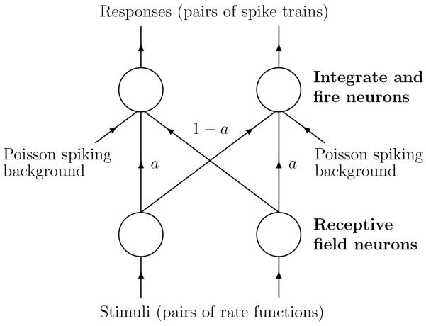
Four neurons are used in the simulation: two receptive neurons feeding forward to two leaky integrate-and-fire (LIF) neurons. The receptive neurons produce Poisson spike trains with time-varying firing rates, the functions determining these firing rates are the analog of stimuli in the simulations and we will refer to a pair of firing rate function as a stimulus. As illustrated in Fig. 1, the feed-forward connectivity depends on a mixing parameter a. Each receptive neuron is connected to one LIF neuron with relative strength a and to the other with relative strength 1 - a. For a = 0 each receptive neuron is connected to a different LIF neuron and for a = 0.5 each LIF neuron receives input equally from each of the receptive neurons. The LIF neurons also receive a background Poisson input. The LIF neurons, in turn, produce spike trains. We will refer to these pairs of spike trains, produced by the LIF neurons, as responses and it is to these that the metrics will be applied. The LIF neurons follow a standard implementation and there is a detailed description of the entire simulation in appendix 2.

Figure 1.

The network used for the simulations. The two receptive neurons produce Poisson spikes according to time varying firing rate functions. These spike trains feed forward to two leaky integrate-and-fire neurons, the relative synaptic strengths of the feed-forward connections are parameterized by a.

During each run, five stimuli are chosen and all five are presented 20 times, giving 100 responses in all. Throughout the simulation and when calculating the new metrics, time is discretized into .25 ms time steps and the stimuli are two seconds long.

4.2 Clustering

To examine the performance of the metrics we will follow the bootstrapped clustering procedure used in (Victor and Purpura, 1996). In this procedure a confusion matrix, N, is calculated; this is a square matrix whose size is given by the number of stimuli and whose ijth entry, N_ij, is the number of responses from stimulus i which are closest, on average, to the responses from stimulus j. Thus, the diagonal entries represent correctly clustered responses and the odiagonal, responses which are closest to the wrong cluster.

More precisely, if there are n responses and c stimuli, the responses are grouped into c clusters according to their stimulus. Starting with all the entries in the confusion matrix set to zero, each response is considered in turn: it is temporarily removed and the average distance between it and the members of each of the c clusters is calculated giving a set of average distances {d₁, d₂, · · · , d_c}. If the smallest distance in this set is d_j and the response being considered was taken from ith cluster, one is added to N_ij. When all the responses have been considered, the elements of N will add to n

$$n=\sum _{i=1}^c\sum _{j=1}^c{N}_{ij}.$$ (24)

In our case, there are five stimuli, so c = 5 and for each stimuli there are 20 responses, so n = 100. As in (Victor and Purpura, 1996), the averaging over cluster elements is performed with a bias exponent, so, for a response r, the biased average distance to the kth cluster, C_k, is

$$d_k={\left[\sum _{s\in C_k}d{(r,s)}^z\right]}^{1∕z}$$ (25)

where the bias is taken to be z = — 2, under-weighting outliers. Of course, here, the responses r and s will be pairs of spike trains and d(r, s) will be one of the multi-unit metrics described above.

If the metric is good at clustering the responses by stimulus, the confusion matrix will be largely diagonal, if it is poor, the entries off the diagonals will be approximately equal to the diagonal elements. As pointed out in (Victor and Purpura, 1996), the transmitted information, h, is a good quantitive measure of how well the responses are clustered. It is given by

$$h=\frac{1}{n}\sum _{ij}{N}_{ij}\left(\ln N_{ij}-\ln \sum _i{N}_{ij}-\ln \sum _j{N}_{ij}+\ln n\right).$$ (26)

For perfect clustering, for c equally likely stimuli, h will be ln c. So, in the case being considered here, the maximum value of h will be ln 5 ≈ 1.61. If there is no clustering by stimulus h = 0, though, in practise, a finite sample will over-estimate this.

4.3 Results

We will use the L¹ version of the new metrics with the block kernel δ_2/q given in Eq. (5). This makes the comparison between the new metric and the ARMV metric clearer: as discussed above, the Victor-Purpura metric with cost parameter q is very similar to the L¹ van Rossum metric with the δ_2/q kernel. A time scale of 2/q = 20 ms is used for the new metrics and with the corresponding q used in the ARMV metrics, this matches the membrane time constant in the LIF neurons. The L¹ version of the new metrics have a parameter α with α = 0 corresponding to the SP metric and α = 1 to LL. The simulations also have a parameter, a, which controls how much the inputs from the two receptive neurons are mixed in the LIF neurons.

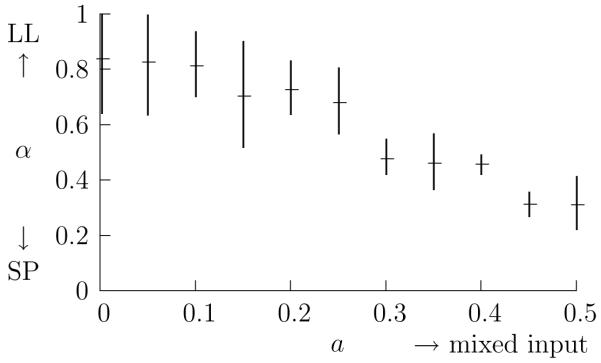
First, we examine whether it is possible that the metric parameter α could be used to deduce the connectivity of neurons from spiking responses. In Fig. 2, the optimal metric parameter, as determined by calculating the transmitted information h (26), is graphed against for different values of a. It is seen that when there is no mixing, a = 0, the best clustering results from α nearer one and, when the inputs are equally mixed, a = 0.5, the best clustering results from values of α nearer zero. Furthermore, the transition between these two is gradual.

Figure 2.

The optimal α plotted against a. The value of metric parameter α giving the maximum h is plotted for different values of the mixing parameter a. For each value of a the best value of α has been found for 20 different runs, the average is marked and the error bars give one standard deviation.

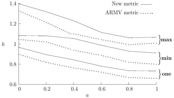
In Fig. 3 the performances of both the new metrics and the ARMV metrics are plotted against a. The new metrics consistently have a higher h value than the ARMV metrics. This implies that, at least on simulated data, the new metrics are better at capturing the structures in the data which encode the stimuli. This should not be taken to imply that the new metrics will prove better than the ARMV metrics when dealing with real data, the simulated data probably has a different statistical structure than real data. It is noteworthy, however, that both metrics have a similar performance profile, changing in a similar way as a changes; this indicates that they have similar clustering properties. The distinction between them is therefore likely to be subtle and informative when applied to real data and, for large numbers of neurons, where the ARMV metrics become computationally expensive, the new metrics are likely to produce similar results.

Figure 3.

The relative performances of the different metrics. The best and worst value of h over the parameter range is plotted against a, the mixing parameter. For each value of a, h was calculated for different values of the metric parameter, α ∊ [0, 1] for the new metric and k ∊ [0, 2] for the ARMV metric. The best and worst values are marked max and min in the graph, the average h value calculated using the responses of each of the two neurons taken on its own is also shown and is marked one. For the single unit examples, the new metric reduces to the van Rossum metric and the ARMV to the Victor-Purpura metric. All values have been averaged over 20 runs.

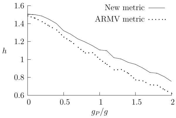
Again, when the performances of the metrics are plotted as the spike trains are degraded, the new metrics outperform the ARMV metrics, and, more importantly, the performance profiles are very similar. In Fig. 4, the h value for metric clustering is plotted as the relative amount of background input is increased. When there is no background input, both the new metric and ARMV metrics have similar performances, near the maximum possible value. As the background input becomes more and more significant, the h value falls. When the amount of background input is five times the feed-forward input from the receptive neurons, h has fallen to 0.75 for the new metric, and 0.62 for the ARMV metric.

Figure 4.

Noise and the performances of the metrics. Here, the amount of input from the Poisson background is varied: h is plotted against the relative value of the synaptic strengths g and g_P for the new and ARMV metrics. For each value of g_P /g, the synaptic strengths were tuned to give the LIF neurons a firing rate of 20 Hz. Because the background spiking has a higher average rate, gP /g = 1 corresponds to an input where the background component is, on average, 2.5 times larger than the component coming from the receptive neurons.

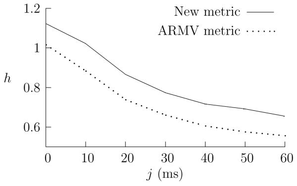
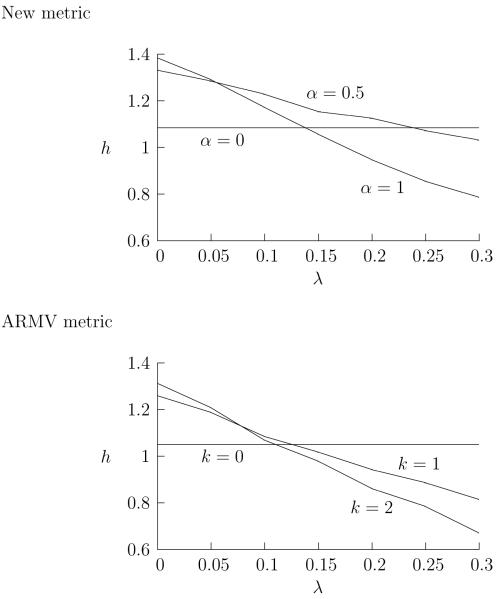
In Fig. 5, the spike trains are degraded by adding jitter; again, as the jitter is increased, the h value falls in a similar way for both the new and ARMV metrics. In Fig. 6 the spike trains are degraded by the random relabelling of individual spikes, this is intended to reproduce the situation where a spike sorting algorithm is used to separate individual spike trains from a single recording. Again, the performances of both metrics decline gracefully. As before the new metric performs better and, in this case, it is more robust.

Figure 5.

Jitter and the performance of the metrics. Jitter has been added to all the spikes in the a = 0.5 simulated responses; the jitter has been drawn uniformly from the interval [-j, j]. In each case, the mixing parameter is a = 0.5; for the new metrics, α = 0.5 and k = 1 for the ARMV metrics. For each value of j, h is averaged over 20 runs.

Figure 6.

Spike misassignment and the performances of the metrics. The spike trains have been corrupted by a random relabelling of the spikes, each spike has a λ probability of being swapped over to the other spike train in the response. For both the new and ARMV metrics, h is plotted against λ for the SP and LL metrics, as well as the metric lying half way between these: α = 0.5 for the new metrics and k = 1 for the ARMV metrics. For each value of λ, the value of h is averaged over 20 runs. The runs are all for zero mixing parameter, a = 0, where the LL metrics are at their greatest advantage over the SP metric. The SP distances are invariant under the relabelling of spikes.

5 Discussion

We have presented new multi-neuron metrics: they are constructed by mapping the multi-neuron spike trains into a space of vector fields. The metrics are straight-forward to calculate. It does not seem possible to say whether the metrics present here or the ARMV metrics presented in (Aronov et al., 2003) will prove more useful for analyzing multi-unit recordings in the primary sensory regions. However, in the case of the simulated data, the two types of metrics perform in a very similar way when the simulation parameters are changed and when the simulated spike trains are degraded. As with the ARMV metrics, it is expected that the new metrics will be a useful tool in analysing the population coding of information in the sensory pathways. It is also hoped that the subtle differences between the new metrics and the ARMV metrics will, when applied to real data, reveal subtle difference in neuronal coding.

The new metrics are faster to compute than the ARMV metrics. In a situation like the one described in section 4, where a large matrix of distances is computed, the slowest step is calculating the distance between the two response vectors fields. This is an O(n²d) calculation, where n is the number of neurons and d is the number of time steps used in the integration. The ARMV metric, in comparison, has computation time O(2n²mⁿ⁺¹) (Aronov, 2003), where m is the typical number of spikes in a spike train. This illustrates one elegant aspect of the ARMV metrics: they can be calculated without discretizing time, however, they are slower. In the simulations we have performed, m = 40, n = 2 and d = 4000 predicting that for two neurons the new metrics are an order of magnitude quicker. This is what we observed when analyzing the simulated data. Even for small numbers of neurons, the new metric is considerably faster and for large numbers of neurons the difference will be huge. Thus the new metrics may provide a useful tool to do template-based spike-train classification for brain-computer interfaces with large numbers of units.

Appendix 1: More than two spike trains

It is easy to generalize the two-neuron metrics to metrics for more than two neurons by using higher-dimensional unit vectors. The multi-neuron metrics have many parameters, corresponding to the different angles between the unit vectors. At first, this may seem to distinguish this family of metrics from the ARMV metrics which are described as having only one such parameter. However, the ARMV metrics can be generalized so that there are different costs for relabelling spikes between different pairs of neurons. Although it is likely that multi-neuron metrics will be most useful when each of these inter-neuronal parameters is separately optimized, it is possible to consider a family of multi-neuron metrics which has only one parameter, by requiring, for example, that the unit vectors are all at the same mutual angle. A set of this sort can be calculated by doing a succession of rotations in different planes. The first unit vector, e¹, is chosen to lie in x₁-direction: (1, 0, · · · , 0), the second, e² is then generated from the first by rotating it an angle θ in the x₁x₂-plane. e³, in turn, is generated from the second by rotating it an angle θ’ in the x₂x₃-plane. Since the x₁-axis is perpendicular to the x₂x₃-plane, e¹ · e³ = e¹ · e² = cosθ. However, θ’ must be chosen to make the angle between the e² and e³ equal to θ. For three-neurons, for example, the three unit vectors would be given by

$${\mathbf{e}}^1=\left(\begin{array}{c}\hfill 1\hfill \\ \hfill 0\hfill \\ \hfill 0\hfill \end{array}\right),{\mathbf{e}}^2=\left(\begin{array}{c}\hfill \cos \theta \hfill \\ \hfill \sin \theta \hfill \\ \hfill 0\hfill \end{array}\right),{\mathbf{e}}^3=\left(\begin{array}{c}\hfill \cos \theta \hfill \\ \hfill \sin \theta \cos {\theta }^{\prime }\hfill \\ \hfill \sin \theta \sin {\theta }^{\prime }\hfill \end{array}\right)$$ (27)

and taking the scalar product of e² and e³ shows that cos θ’ is given by

$$\cos {\theta }^{\prime }=\frac{\cos \theta -{\cos }^2\theta }{{\sin }^2\theta }$$ (28)

and, of course, $\sin {\theta }^{\prime }=\sqrt{1-{\cos }^2{\theta }^{\prime }}$,θ’ itself is not needed. For four neurons, a further rotation in the x₃x₄-plane gives unit vectors

$$\left(\begin{array}{c}\hfill 1\hfill \\ \hfill 0\hfill \\ \hfill 0\hfill \\ \hfill 0\hfill \end{array}\right),\left(\begin{array}{c}\hfill \cos \theta \hfill \\ \hfill \sin \theta \hfill \\ \hfill 0\hfill \\ \hfill 0\hfill \end{array}\right),\left(\begin{array}{c}\hfill \cos \theta \hfill \\ \hfill \sin \theta \cos {\theta }^{\prime }\hfill \\ \hfill \sin \theta \sin {\theta }^{\prime }\hfill \\ \hfill 0\hfill \end{array}\right),\left(\begin{array}{c}\hfill \cos \theta \hfill \\ \hfill \sin \theta \cos {\theta }^{\prime }\hfill \\ \hfill \sin \theta \sin {\theta }^{\prime }\cos {\theta }^{\prime \prime }\hfill \\ \hfill \sin \theta \sin {\theta }^{\prime }\sin {\theta }^{\prime \prime }\hfill \end{array}\right)$$ (29)

where

$$\cos {\theta }^{\prime \prime }=\frac{\cos {\theta }^{\prime }-{\cos }^2{\theta }^{\prime }}{{\sin }^2{\theta }^{\prime }}$$ (30)

and, in fact, this can be iterated: in going from the n - 1 neuron to the n neuron case, the extra unit vector can be obtain by a rotation into the new dimension by an angle that satisfies an equation of this form.

Appendix 2: The simulation

The receptive neurons fire stochastically, with a time dependent firing rate given by a rate function, s(t). These rate functions are chosen randomly as rectified Fourier series:

$$s\left(t\right)=A{\left[\sum _{i=0}^{20}{a}_n\cos 2n\pi t∕T\right]}_{+}$$ (31)

where T = 2s is the total duration of the stimulus and the a_n are sampled uniformly from the interval [ — 1, 1]. The square bracket denotes half-wave rectification

$${\left[x\right]}_{+}=\{\begin{array}{cc}x\hfill & x>0\hfill \\ 0\hfill & \text{otherwise}\hfill \end{array}\phantom{\}}$$ (32)

and A is chosen so that

$${\int }_0^{T}s\left(t\right)=20T$$ (33)

giving an average firing rate of 20 Hz.

For the LIF neurons, a standard model is used, following an example described in (Dayan and Abbott, 2001). Each neuron has a voltage satisfying

$${\tau }_m\frac{dV}{dt}=E_l-V+I$$ (34)

where E_l = — 54mV is the leak potential, τ_m = 20 ms is the membrane time constant and I is the synaptic input current. The neuron fires when V reaches the threshold, — 50 mV and is then reset to — 65 mV. The synaptic current is

$$I=g(E_e-V)$$ (35)

where E_e = 0 mV is the excitatory synapse reversal potential; all the synapses are excitatory. The synaptic conductance is the sum of the individual synaptic conductances. For each LIF neuron there are three synapses, two feeding forward from the receptive neurons and one from the background. In each case the synaptic conductance depends on a gating probability P and is given by g_maxP where g_max = ga and g(1 - a)for the feed-forward synapses, with g = 1.25 and g_max = gp for the background synapse.

These values have been chosen to give the LIF neurons spiking rates of roughly 20 Hz, though the precise value will vary from stimulus to stimulus. Each synapse has its own gating probability P satisfying

$${\tau }_s\frac{dP}{dt}=-P$$ (36)

where τ_s = 4 ms is the synaptic time constant. Each time a spike arrives at a synapse, that synapse’s gating probability is increased according to

$$P\to P+(1-P)P_{\max }$$ (37)

where P_max = 0.3.

For most simulations gp = g; the only time g and g_P are varied is in the simulations used to produce Fig. 4 where the e ect of changing the ratio gP /g is examined. The background firing rate is 50 Hz. So, for g_P = g, the average input current from the background is 2.5 times the average current from the receptive neurons, however, the variance of the current from the receptive neurons will be much higher.

References

- Aronov D. Fast algorithm for the metric-space analysis of simultaneous responses of multiple single neurons. Journal of Neuroscience Methods. 2003;124:175–179. doi: 10.1016/s0165-0270(03)00006-2. [DOI] [PubMed] [Google Scholar]
- Aronov D, Reich DS, Mechler F, Victor JD. Neural coding of spatial phase in v1 of the macaque monkey. Journal of Neurophysiology. 2003;89:3304–3327. doi: 10.1152/jn.00826.2002. [DOI] [PubMed] [Google Scholar]
- Dayan P, Abbott LF. Theoretical Neuroscience. MIT Press; 2001. [Google Scholar]
- Kreuz T, Haas JS, Morelli A, Abarbanel HDI, Politi A. Measuring spike train synchrony. Journal of Neuroscience Methods. 2007;165:151–161. doi: 10.1016/j.jneumeth.2007.05.031. [DOI] [PubMed] [Google Scholar]
- Narayan R, Graña G, Sen K. Distinct time scales in cortical discrimination of natural sounds in songbirds. Journal of Neurophysiology. 2006;96:252–258. doi: 10.1152/jn.01257.2005. [DOI] [PubMed] [Google Scholar]
- Schreiber S, Fellous JM, Whitmer D, Tiesinga P, Sejnowski TJ. A new correlation-based measure of spike timing reliability. Neurocomputing. 2003;52-54:925–931. doi: 10.1016/S0925-2312(02)00838-X. [DOI] [PMC free article] [PubMed] [Google Scholar]
- van Rossum M. A novel spike distance. Neural Computation. 2001;13:751–763. doi: 10.1162/089976601300014321. [DOI] [PubMed] [Google Scholar]
- Victor JD, Purpura KP. Nature and precision of temporal coding in visual cortex: a metric-space analysis. Journal of Neurophysiology. 1996;76:1310–1326. doi: 10.1152/jn.1996.76.2.1310. [DOI] [PubMed] [Google Scholar]
- Victor JD, Purpura KP. Metric-space analysis of spike trains: theory, algorithms and application. Network: Computation in Neural Systems. 1997;8:127–164. [Google Scholar]