Abstract
In functional magnetic resonance imaging (fMRI), the process of determining statistically significant brain activation is commonly performed in terms of voxel time series measurements after image reconstruction and magnitude-only time series formation. The image reconstruction and statistical activation processes are treated separately. In this manuscript, a framework is developed so that statistical analysis is performed in terms of the original, pre-reconstruction, complex-valued k-space measurements. First, the relationship between complex-valued (Fourier) encoded k-space measurements and complex-valued image measurements from (Fourier) reconstructed images is reviewed. Second, the voxel time-series measurements are written in terms of the original spatio-temporal k-space measurements utilizing this k-space and image relationship. Finally, voxel-wise fMRI activation can be determined in image space in terms of the original k-space measurements. Additionally, the spatio-temporal covariance between reconstructed complex-valued voxel time series can be written in terms of the spatio-temporal covariance between complex-valued k-space measurements. This allows one to utilize the originally measured data in its more natural, acquired state rather than in a transformed state. The effects of modeling preprocessing in k-space on voxel activation and correlation can then be examined.
Keywords: image reconstruction, k-space, fMRI, complex data, Rowe-Logan
1. Introduction
In functional magnetic resonance imaging (fMRI), an array of data for an individual image is observed in an encoded form. The sampled data are generally Fourier encoded [2,4] and thus are measured spatial frequencies. These spatial frequency (k-space) observations are then reconstructed into an individual image array by the process of an inverse Fourier transformation. A series of these arrays of encoded images are acquired and the reconstruction process is applied to each array. For each voxel, temporally sequential voxel measurements are collected into a time series for determination of statistically significant activation. The originally sampled spatial frequencies are complex-valued and the inverse Fourier transformation image reconstruction process may yield complex-valued data. Due to measurement error and imperfections in the Fourier encoding, voxel time series are generally complex-valued.
The process of determining statistical activation in each voxel has, for the most part, been from magnitude-only time series [1,12]. The process of converting a complex-valued time series into a magnitude-only time series is to take the square root of the sum of the squares of the real and imaginary parts of the complex-valued time series at each time point [11]. An activation statistic from the magnitude-only time series for each voxel is determined by computing a measure of association between the observed voxel time series and a preassigned ideal time series based on the timing of the experiment and physiological considerations. This association measure for each voxel is statistically compared to the association measure that would result from a time series of random noise. A statistical threshold is chosen, a scale of color values for the activation statistic is assigned, and each voxel above threshold is given the color corresponding to its activation statistic.
The idea of computing an activation statistic from the complex-valued time series has been previously discussed [5,8]. This idea of computing fMRI activation from complex-valued data has recently been expanded upon [9-12]. Work has also been performed on computing fMRI activation from phase-only time series [13]. However, the processes of image reconstruction and statistical activation have been treated separately. Thus, activation is determined in terms of complex-valued voxel measurements after reconstruction and not the original encoded measurements.
In the current study, the relationship between the original encoded k-space measurements and reconstructed voxel measurements for each image is summarized. For each image, a vector of real-imaginary reconstructed voxel measurements is formed and written as a linear combination of real-imaginary k-space measurements. A larger vector of reconstructed real-imaginary voxel time series measurements is formed by stacking the individual vectors of real-imaginary voxel measurements for each image in temporal order. This large vector is written as a linear combination of a large vector of real-imaginary k-space time series measurements that is ordered in a similar manor. A permutation matrix is utilized to reorder the voxel measurements that are real then imaginary per image to be of real then imaginary per voxel. Statistical functional brain activation can then be determined with the aforementioned recent complex-valued activation models. A map of these activation statistics can then thresholded to determine statistically significant activation while adjusting for multiple comparisons [6,7].
Statistically significant voxel activation and correlation between voxels can thus be determined in image space in terms of the originally acquired k-space measurements. This will allow the modeling of the originally acquired measurements in their original state, as they are acquired, and not in a transformed state. Implications of k-space preprocessing on voxel activation and correlation can then be evaluated.
2. Background
Previous work has included the development of a real-valued representation of the standard complex-valued Fourier transform [14]. In this section we review the representation and offer a graphical example to illustrate the method. Magnetic resonance images are almost exclusively Fourier encoded. That is, one ideally measures the Fourier transform of an image and reconstruct the image via an inverse Fourier transform. The Fourier transform and inverse Fourier transforms are complex-valued procedures that results in complex-valued arrays.
Standard, complex-valued Fourier matrices are defined as follows. If ΩC is a p×p Fourier matrix, it is a matrix with (j,k)th element [ΩC]jk= κ (ωjk) where κ=1 and ω=exp[-i 2 π (j-1)(k-1)/p] for the forward transformation while κ=1/p and ω =exp[+i 2π (j-1)(k-1)/p] for the inverse transformation, where j,k=1,…,p.
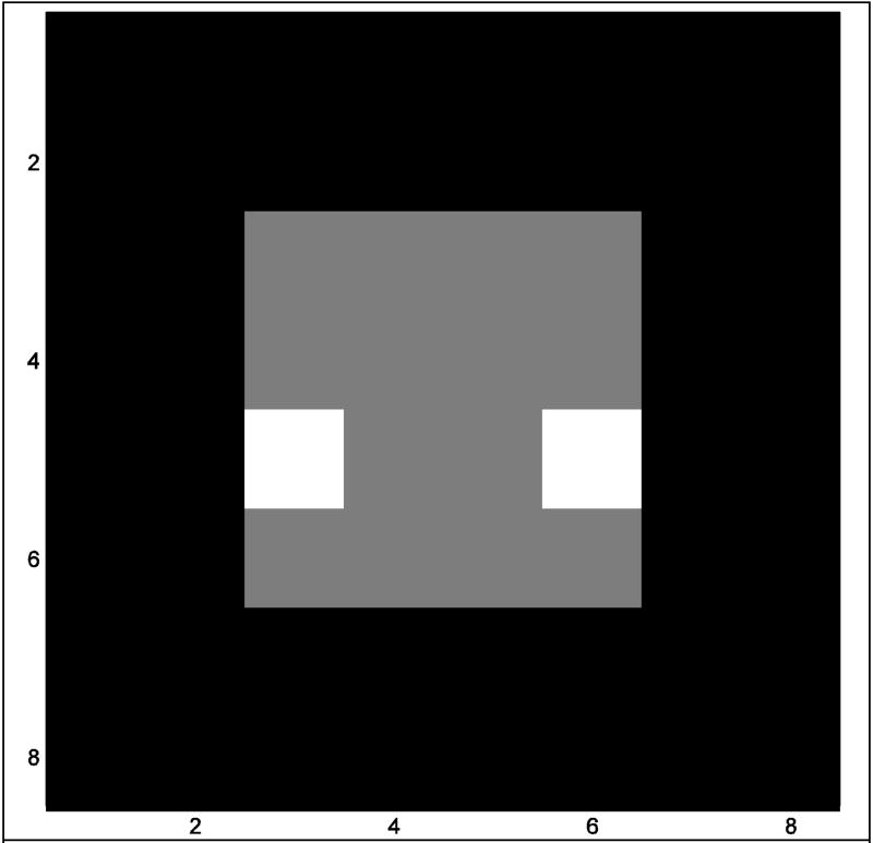
Consider the Fourier transform of an image that has dimensions py×px(py rows and px columns). Often the image is square, although this is not necessary. More specifically, consider an 8×8, ideal, noiseless, gray scale image as presented in Fig. 1. Since the Fourier transform and inverse Fourier transform procedures operate on, and produce complex-valued arrays, the real-valued image in Fig. 1 can be represented as a complex-valued image RC that has a real part RR as in Fig. 1 an imaginary part RI that is the zero matrix so that RC=RR+iRI. The encoded data, or Fourier transform of this image, can be found as in Eq. (1) by pre-multiplying the py×px dimensional complex-valued matrix RC by a standard complex-valued forward Fourier matrix Ω̄yC=Ω̄yR+iΩ̄yI, that is of dimensions py×py, and post-multiplying RC by the transpose of another standard forward Fourier matrix , where T denotes matrix transposition, that is of dimensions px×px. The result of the pre- and post-multiplications is a complex-valued array of spatial frequency (k-space) measurements, SC, with real part SR and imaginary part SI as also shown in Eq. (1).
Fig. 1.
Ideal noiseless image.
| (1) |
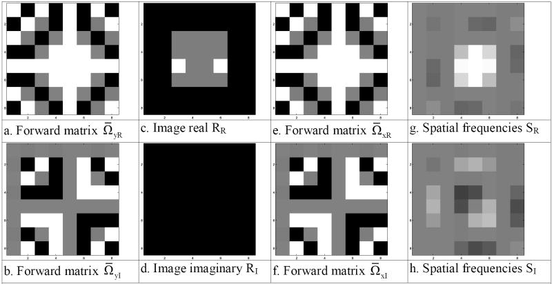
This mathematical procedure is graphically illustrated in Fig. 2 using the aforementioned 8×8 image. In Fig. 2 the 8×8 image, RC, is utilized to mimic an image from a magnetic resonance echo planar imaging experiment. RC is displayed with real part, RR, in Fig. 2c and imaginary part, RI, in Fig. 2d. The spatial frequency (k-space) values, SC=(SR+iSI), associated with this complex-valued image, are found by pre-multiplying the complex-valued image by the complex-valued forward Fourier matrix Ω̄yC (Fig. 2a and Fig 2b) and then post-multiplying the result by the transpose of the symmetric forward Fourier matrix (Fig. 2e and Fig. 2f). The spatial frequency (k-space) values, SC, for the complex-valued image RC are presented as an image with real part, SR, in Fig. 2g and imaginary part, SI, in Fig. 2h. Note that, as mentioned earlier, the image does not have to be square.
Fig. 2.
- Forward matrix Ω̄yR
- Forward matrix Ω̄yI
- Image real RR
- Image imaginary RI
- Forward matrix Ω̄xR
- Forward matrix Ω̄xI
- Spatial frequencies SR
- Spatial frequencies SI
However, as previously described, in MRI encoded (k-space) measurements, SC, are made and reconstructed (transformed) into an image. The inverse Fourier procedure is performed. This reconstruction procedure, or inverse Fourier transform, of the spatial frequency (k-space) measurements can be found as
| (2) |
by pre-multiplying the py×px dimensional complex-valued spatial frequency matrix, SC, by a complex-valued inverse Fourier matrix, Ωy, that is of dimensions py×py, and post-multiplying SC by the transpose of another Fourier matrix, Ω̄xT, that is of dimensions px×px, where T denotes matrix transposition. The result of the pre- and post-multiplications is a complex-valued array of image measurements RC, with real part RR and imaginary part RI as also shown in Eq. (2).
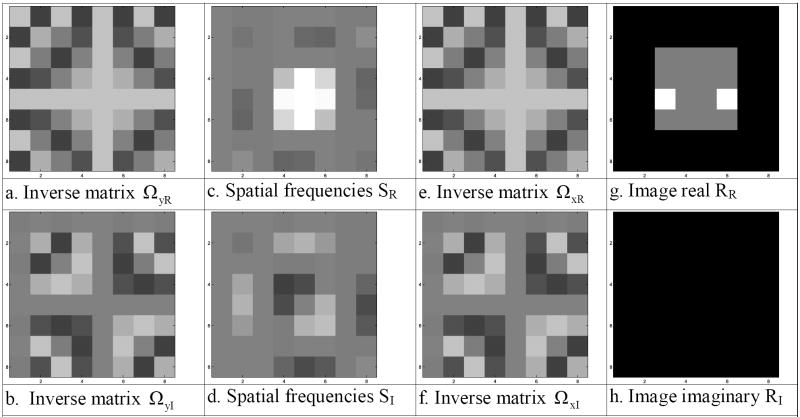
The complex-valued image RC can be recovered as seen in Fig. 3. The process of recovering the original complex-valued image RC is to pre-multiply the complex-valued spatial frequency (k-space) values SC by the complex-valued inverse Fourier matrix ΩCy, (Fig. 3a and Fig. 3b) then post-multiply the result by the transpose of the symmetric inverse Fourier matrix ΩCx, (Fig. 3e and Fig. 3f). The recovered complex-valued image, RC, is presented with real part, RR, in Fig. 3g and imaginary part, RI, in Fig. 3h.
Fig. 3.
- Inverse matrix ΩyR
- Inverse matrix ΩyI
- Spatial frequencies SR
- Spatial frequencies SI
- Inverse matrix ΩxR
- Inverse matrix ΩxI
- Image real RR
- Image imaginary RI
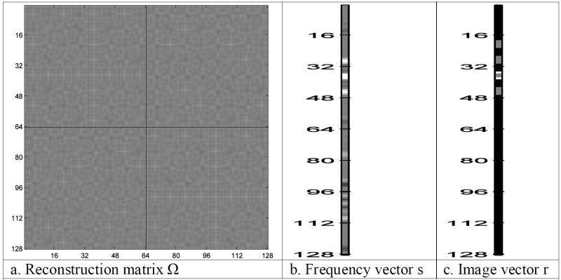
This complex-valued inverse Fourier transformation image reconstruction process can be equivalently described as a linear transformation with a real-valued representation [14]. Such a transformation is often called an isomorphism in mathematics. Define a real-valued vector, s, to be a 2pxpy dimensional vector of complex-valued spatial frequencies from an image where the first pxpy elements are the rows of the real part of the spatial frequency matrix, SR, shown in Fig. 3c, and the second pxpy elements are the rows of the imaginary part of the spatial frequency matrix, SI, shown in Fig. 3d. The real-valued vector of spatial frequencies is thus formed as s=vec(SRT,SIT), where (SRT,SIT) is a px×2py matrix formed by joining the transpose of the real and imaginary parts of SC as seen in Fig. 4a, and vec(·) denotes the vectorization operator that stacks the columns, shown in Fig. 4b, of its matrix argument. This yields us a real-valued vector representation of the matrix of spatial frequency (k-space) values that is given in Fig. 5b.
Fig. 4.
- Spatial frequencies ST=(SRT,SIT)
- Partitioned spatial frequencies ST
Fig. 5.
- Reconstruction matrix Ω
- Frequency vector s
- Image vector r
Further define a matrix Ω that is another representation of the complex-valued inverse Fourier transformation matrices as described in Eq. (3) where the matrix elements of Ω are
and ⊗ denotes the Kronecker product that multiplies every element of its first matrix argument by its entire second matrix argument. Utilizing the complex-valued Fourier matrix ΩCy, with real and imaginary parts ΩyR and ΩyI given in Fig. 3a and Fig. 3b, along with the complex-valued Fourier matrix ΩCx, with real and imaginary parts ΩxR and ΩxI given in Fig. 3e and Fig. 3f, the resulting Ω matrix is presented in Fig. 5a.
The real-valued vector representation s of the spatial frequency (k-space) values in Fig. 5b is then pre-multiplied by the (inverse Fourier) reconstruction matrix Ω as in Eq. (3)
| (3) |
where the real-valued representation, r, of the complex-valued image has a dimension of 2pxpy×1, true mean and no measurement error.
This is pictorially represented in Fig. 5. Fig. 5b is the spatial frequency vector s and Fig. 5a is the inverse Fourier transformation matrix Ω as described in Eq. (3). This matrix multiplication produces a vector representation, r, of the image voxel measurements given in Fig. 5c as described in Eq. (3). The vector of voxel measurements, r, is partitioned into column blocks of length px. These blocks are then arranged as in Fig. 6a and formed into a single matrix image as in Fig. 6b where the first (last) eight columns are the transpose of the real (imaginary) part of the image. As can be seen, the same resultant complex-valued image is reconstructed with the complex-valued inverse Fourier transformation procedure described in Eq. (2) and presented in Fig. 3.
Fig. 6.
- Partitioned images RT
- Combined image RT=(RRT, RIT)
In the above described procedure, measurement noise was not considered. Redefine SC to be the py×px dimensional complex-valued spatial frequency measurement of a slice with noise that consists of a py×px dimensional matrix of true underlying noiseless complex-valued spatial frequencies, S0C, and a py×px dimensional matrix of complex-valued measurement error, EC. This partitioning of the measured spatial frequencies in terms of true noiseless spatial frequencies plus measurement error can be represented as
| (4) |
where i is the imaginary unit while S0R, S0I, ER, and EI are real and imaginary matrix valued parts of the true spatial frequencies and measurement noise, respectively. Let ΩCx and ΩCy be px×px and py×py complex-valued Fourier matrices as described above. Then, the py×px complex-valued inverse Fourier transformation reconstructed image, RC, of SC can be written as
| (5) |
where RC has a true mean R0C and measurement error NC. Note that the complex-valued matrices for reconstruction, Ωx and Ωy in Eq. (5), need not be exactly Fourier matrices but may be Fourier matrices that include adjustments for independently measured magnetic field inhomogeneities or reconstruction matrices for other encoding procedures.
The real-valued inverse Fourier transformation method for image reconstruction can also be directly applied to noisy measurements. We can represent the noisy complex-valued spatial frequency matrix as s=s0+ε where this 2pxpy dimensional vectors includes the reals of the rows stacked upon the imaginaries of the rows of the corresponding matrix. This implies that if the mean and covariance of the spatial frequency measurement vector, s, that is of dimension 2pxpy×1, are s0 and Γ, then the mean and covariance of the reconstructed voxel measurements, r, are Ωs0 and ΩΓΩT.
3. Theory
The previously described data for a single image is expanded upon to mimic an fMRI experiment. In fMRI, a series of the previously described image slices are acquired. Denote the py×px complex-valued spatial frequency matrix, corrupted by random noise, acquired at time t as SCt=S0Ct+ECt and define , where SRt and SIt are the real and imaginary parts of SCt for time points t=1,…,n. Define the total number of voxels in the image, which is the same as the number of complex-valued k-space measurements in fully sampled, Fourier encoded, Cartesian acquisitions, to be p=pxpy. This sequence of measured spatial frequency vectors can be collected into a 2p×n matrix S=(s1,…,sn) where the tth column contains the p real k-space measurements stacked upon the p imaginary k-space measurements for time t. Having done this, n reconstructed images can be formed by the 2p×n matrix R=ΩS where the tth column of R contains the p real voxel measurements stacked upon the p imaginary voxel measurements for time t, t=1,…,n.
The k-space measurements and the image voxel measurements can be stacked as s=vec(S) and r=vec(R). Note that s and r and have been redefined from their initial definition. If the mean and covariance of the 2np×1 vector of spatial frequency measurements, s, are s0 and Δ, then the mean and covariance of the 2np×1 vector of reconstructed voxel measurements, r, are (In ⊗ Ω)s0 and (In ⊗ Ω)Δ(In ⊗ ΩT). For example, if the k-space measurements were taken to be temporally independent, then Δ=In ⊗ Γ and cov(r)=In ⊗ (ΩΓΩT), where Γ is the covariance matrix for one k-space acquisition. Thus, we have described the fMRI voxel measurements as a linear function of the fMRI k-space measurements.
We can alternatively organize the voxel measurements by stacking the first set of p columns of RT upon the second set of p columns of RT to form a matrix Y of dimension 2n×p. Having done this, the jth column of the resulting data matrix Y contains the n real voxel measurements stacked upon the n imaginary voxel measurements for voxel j, j=1,…,p. The voxel measurements Y can be described with the complex fMRI model [12] as
| (6) |
where C1 and S1 are diagonal matrices with cosine and sine terms respectively. Different activation models are found from Eq. (6) by different choices of the C and S matrices. The complex constant phase model [11] can be found with Cj=Incosθj and Sj=Insinθj where j indexes the jth voxel. The unrestricted phase or magnitude only model can be found by selecting the tth element of Cj and Sj to be Cjt=cosθjt and Sjt=sinθjt, where θjt is unique for each j and t. The complex model for both magnitude and phase [9] can be found by choosing the phase θjt= utTγj where ut is the tth row of a phase design matrix U and γj are phase regression coefficients for voxel j.
Equation 6 can be rearranged and written with y=vec(Y) as
| (7) |
where is a vector containing the real and imaginary reconstructed voxel measurements and is a vector containing the real and imaginary errors of the reconstructed voxel measurements. The model can simply be written as y=μ+ε. For example, with constant phase model, the mean is
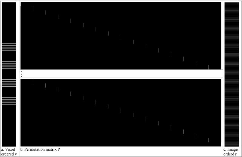
The rearrangement of the voxel measurements from r to y is a linear transformation and can be achieved through multiplication with a permutation matrix P (described in Appendix A and presented in Fig. 10) as y=Pr. In terms of the original k-space measurements the voxel time courses are . Having done this linear transformation, the mean and covariance of y are μ=P(In ⊗ Ω)s0 and Λ=P(In ⊗ Ω)Δ(In ⊗ ΩT)PT. Since the matrices Ω and P that convert k-space measurements, s, to voxel measurements, y, are known a priori, the expression y=P(In ⊗ Ω)s can be inverted to write s= (In ⊗ Ω-1)P-1y, and in terms of the parameters as
Fig. 10.
- Voxel ordered y
- Permutation matrix P
- Image orderd r
| (8) |
Thus the optimization for the regression coefficients (β) and phases (θ) in Eq. (8) can be performed in k-space to yield the same parameter estimates as the standard method. Activations can then be computed from the described complex activation models.
Using ordinary least squares or a normal distributional specification on the errors, the voxel-wise regression coefficients and phases can be determined to yield the same point estimators as in Rowe and Logan [11]. The Rowe-Logan unconstrained alternative hypothesis estimators (with hats) for H1:Cβ≠0 along with the constrained null hypothesis estimators (with tildes) for H0:Cβ=0 in voxel j are
| (9) |
where C is an r×(q+1) matrix of full row rank, ψ=Iq+1-(XTX)-1CT[C(XTX)-1CT]-1C, β̂Rj=(XTX)-1XTyRj, and β̂Ij=(XTX)-1XTyIj, while yRj and yIj are the n×1 vectors of real and imaginary voxel observations.
We can convert from the vector r, which is presented in Fig. 10c, to the vector y, which is shown in Fig. 10a, via a permutation matrix P, a portion of which is displayed in Fig. 10b. Now with the y vector being arranged as real and imaginary observations in each voxel as described in Eq. (7), we can apply the complex activation models [11]. The regression coefficients β, the phase angle θ, and the variance σ2 are estimated under both the null and alternative hypotheses as described in Eq. (9) then activation computed.
Voxel-wise activations are the same as in Rowe and Logan [11]. Then the generalized likelihood ratio statistic for the complex fMRI activation model is . This statistic has a large sample χr2 distribution. Note that when r=1, two-sided testing can be done using the signed likelihood ratio test given by
| (10) |
which has a large sample standard normal distribution under the null hypothesis. Alternatively with r=1, a Wald type statistic can be formed
| (11) |
which also has a large sample standard normal distribution under the null hypothesis. A map of these activation statistics from either Eq. 10 or Eq. 11 is then thresholded while adjusting for multiple comparisons [6,7]. However, correlations between voxels are characterized in terms of spatio-temporal correlations between k-space measurements.
The variances and covariances in the spatio-temporal domain in an example with a specification of uncorrelated temporal k-space measurement vectors (st) are included in the covariance matrix Λ=P(In ⊗ ΩΓΩT)PT for the voxel measurements. Define the voxel measurement covariance matrix to be Σ. Having estimated the voxel-wise regression coefficients and phases, we can estimate the mean of the vector of voxel measurements y by μ̂ (under the alternative hypothesis) and the mean of the matrix of voxel measurements R by M̂=vec̅(P-1μ̂). Here vec̅(·) is the operator that is the inverse operation of the vec(·) operator. The voxel covariance matrix Σ can now be estimated by Σ̂=(R-M̂)(R-M̂)T/n.
With the physically motivated specification of the same voxel covariance, ΣW, within the real-imaginary channels and voxel covariance, ΣB, between the real-imaginary channels, the previous the voxel covariance matrix becomes
| (12) |
We can estimate the covariance matrices in Eq. (12) under the alternative hypothesis by
| (13) |
and under the null hypothesis similarly find Σ̃W and Σ̃B by replacing hats in Eq. (13) with tildes. It should be noted that the jth diagonal elements of Σ̂W are equivalent to those given in Rowe and Logan [11] where the estimate under the alternative hypothesis is
| (14) |
and under the null hypothesis is similarly, σ̃j2 found by replacing hats in Eq. (14) with tildes. As described in Eq. (13), we can also estimate covariance between voxels, Σ̂.
4. Methods
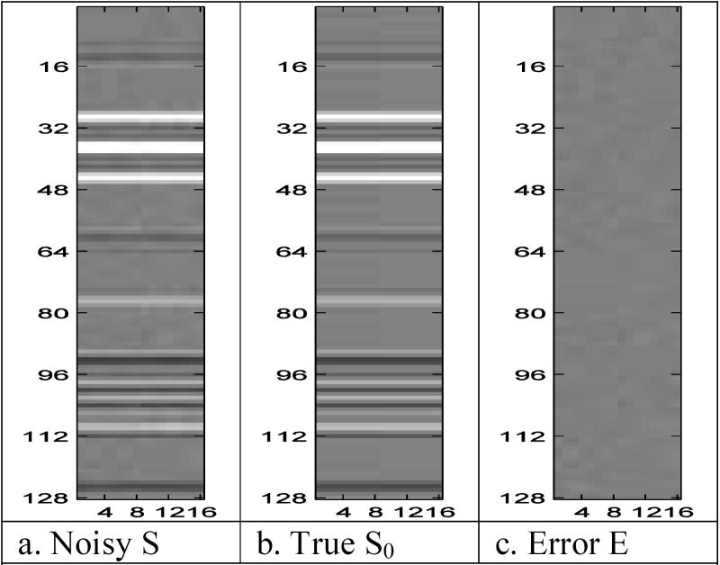
As before, this time series procedure can be represented pictorially. The complex-valued image in Fig. 2c and Fig. 2d was taken as the mean “active” or “on” image and a duplicate of it with the two white voxels replaced by grey voxels were used as the mean “inactive” or “off” images. For illustrative purposes, an experiment with eight blocks where each block consists of eight on images followed by eight off images is initially presented. Subsequently all eight blocks were examined. Eight column vectors of the spatial frequencies for the true mean “on” image were joined into a matrix with eight column vectors of the spatial frequencies for the true mean “off” image as in Fig. 7b. Each column in Fig. 7b is the vector form of the spatial frequencies for an image similar to that in Fig. 5b.
Fig. 7.
- Noisy S
- True S0
- Error E
The mean “on” images contained voxels with values β0=0 and β1=0 outside a four by four by four internal region, inactive gray voxels within the four by four region with values β0=SNR·σ and β1=0, along with two active voxels with value β0=SNR·σ and β1=CNR·σ. Activation parameter values were SNR=30, CNR=1 and σ=.05. In this parameterization, SNR denotes the temporal signal-to-noise ratio, CNR denotes the functional contrast-to-noise ratio, and σ denotes the voxel standard deviation.
Independent noise column vectors εt, as seen in Fig. 7c, were generated from a normal distribution with zero mean vector and covariance matrix Γ=γ2Γ1 ⊗ Γ2 ⊗ Γ3. This covariance structure mimics temporal autocorrelation along the echo planar imaging (EPI) trajectory along with correlation between real and imaginary parts. The covariance matrix was formed with Γ1, Γ2, and Γ3 taken to be unit variance correlation matrices while γ was taken to be γ2=pxpyσ2. The py×py correlation matrix Γ1 is taken to be an AR(1) correlation matrix with (i,j)th element where ψ1 =0.25, the 2×2 correlation matrix Γ2 is taken to have an off diagonal correlation of ψ2 =0.5 while the px×px correlation matrix Γ3 is taken to be an AR(1) correlation matrix with (i,j)th element where ψ3=0.5.
5. Results
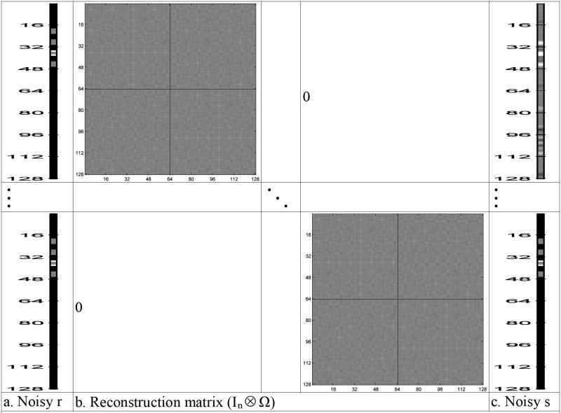
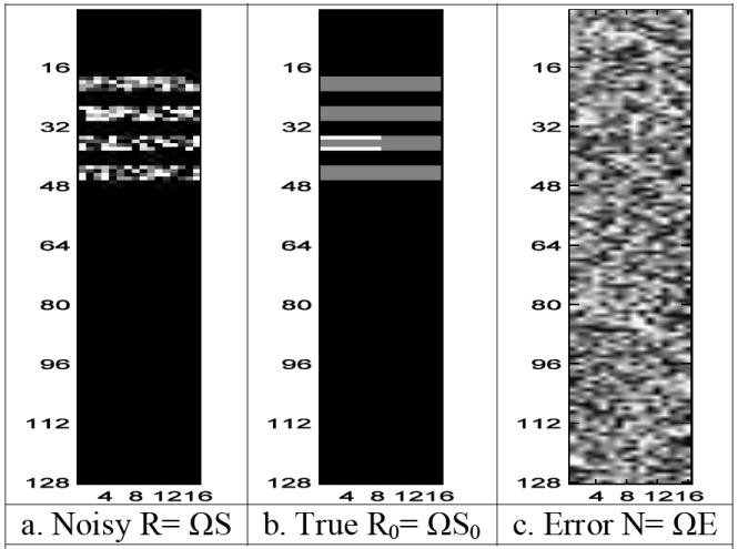
Each matrix image in Fig. 7a, b, and c was pre-multiplied by the (inverse Fourier transform) image reconstruction matrix Ω, given in Eq. (3) and presented in Fig. 5a. The results of this pre-multiplication can be seen in Fig. 8a, b, and c. The columns of R= ΩS in Fig. 8a are real and imaginary parts for each noisy image. The noisy image in Fig. 8a is the sum of the noiseless image in Fig. 8b and the measurement noise image in Fig. 8c. However, the real and imaginary parts for each noisy voxel are useful for considering activation. As described in Section 3, one can vectorize R and S to yield r=vec(R) and s=vec(S) as seen in Fig. 9. The vector s of noisy spatial frequency (k-space) values, as presented in Fig. 9c, is pre-multiplied by a block diagonal matrix with Ω along the diagonal, as displayed in Fig. 9b, to produce a vector of noisy image measurements, r, as shown in Fig. 9a.
Fig. 8.
- Noisy R= ΩS
- True R0= ΩS0
- Error N= ΩE
Fig. 9.
- Noisy r
- Reconstruction matrix (In ⊗ Ω)
- Noisy s
In Fig. 11a and Fig. 11c are the unthresholded activation maps for the magnitude-only and complex-valued activation methods respectively. In Fig. 11b and d are the Bonferroni 5% thresholded activation maps for the magnitude-only and complex-valued activation techniques respectively. Note the spurious activation from the magnitude-only method as a result of its suboptimal parameterization [9].
Fig. 11.
- Magnitude unthresholded
- Magnitude thresholded
- Complex unthresholded
- Complex thresholded
The sample voxel correlation from Σ̂W described in Eq. (13) is displayed in Fig. 12a with theoretical values presented in Fig. 12b. The sample correlation from Γ̂=Ω-1 Σ̂(ΩT)-1 is given in Fig. 12c with theoretical values in Fig. 12d. Note the similarity between the sample values and the theoretical values in Fig. 11a and Fig. 11c to the theoretical values in Fig. 11b and Fig. 11d even for the small sample size.
Fig. 12.
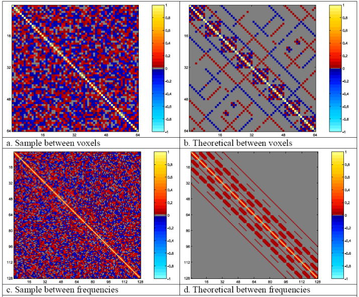
- Sample between voxels
- Theoretical between voxels
- Sample between frequencies
- Theoretical between frequencies
6. Discussion
A linear representation of image reconstruction has been presented, and that reconstruction operation has been included into the complex-valued general linear model for fMRI. This parameterization of the complex-valued general linear model allows one to compute activations directly from k-space measurements. This offers some advantages. The previously separate, tedious processes of image reconstruction and functional analysis can now be considered in one step. As the reconstruction matrix, permutation matrix, and design matrix (marked “known” in Equation 8) are all known, their product may be computed once for a given experiment. Thus, the determination of image-space regression coefficients can be made with one matrix multiplication on the acquired k-space data vector.
Of course, some data processing is more naturally performed in image-space. An example of such processing is motion correction. In that case, a matrix which shifts and/or rotates the reconstructed image can be used to multiply the reconstruction operator. Thus, the processed and reconstructed data would be the result of two matrices multiplying the acquired k-space data in this linear representation.
Furthermore, in light of this parameterization, the spatio-temporal covariances between the complex-valued voxel measurements, Λ, can now be described in terms of the spatio-temporal covariances between the complex-valued k-space measurements, Δ. The covariance of the complex-valued k-space measurements may be due to independent sources, such as spatio-temporal independent noise ΔI and true physiologic processes ΔP, so that Δ=ΔP+ΔI. Adjustments to the k-space measurements could modify the correlation structure. These k-space adjustments can be written as sA=As=A(s0+ε)= As0+Aε and rA=ΩA(s0+ε)= ΩAs0+ΩAε where the subscript A denotes an adjusted measurement. Then the mean and variance/covariance matrices are E(sA)=As0 and var(sA)=AΓAT for the spatial frequency measurements and E(rA)=ΩAs0 and var(rA)=ΩAΓATΩT for the voxel measurements. So unless Γ=I and AAT=I the voxels are correlated because ΩΩT=I. Through reconstruction and other processing, one is changing the physiologic and independent correlations. They change according to
It is possible that incomplete consideration of correlations induces undesirable correlations or obscures relevant correlations. Proper modeling suggests that one should adjust the covariance matrices in light of all data processing.
One could apply temporal filtering or pre-whitening to the k-space measurements that are residuals after fitting a regression model in image space. After fitting the fMRI model to the voxel image time courses, one can transform the residual images into spatial frequencies (k-space) and estimate the correlation due to adjustment sources AAT. The spatial frequencies can then be temporally pre-whitened, transformed back into residual images then the noise variation ΣW re-estimated.
As mentioned earlier, although only Cartesian Fourier reconstruction is described in this manuscript, any linear reconstruction method may be used in place of Ω. This includes non-Cartesian sampling schemes, like spiral. Some new reconstruction operator, ω, may be considered that is the product of two matrices which grid the data to the Cartesian grid and Fourier transform the Cartesian data. Sparsely sampled, multi-coil data may be considered with yet another reconstruction operator, ω’, which generates the omitted data as a linear combination of the acquired multi-coil data and Fourier transforms the generated, fully sampled data.
In this work, complex-valued voxel measurements have been written in terms of the original complex-valued k-space measurements. This allows the computation of statistically significant fMRI brain activation in image space directly from the original k-space measurements. The correlation between voxel measurements can also be written in terms of correlation between k-space measurements. Since the covariance matrix between the k-space measurements, and hence voxel measurements, can be partitioned into individual sources of covariation, statistical associations between individual voxels or regions of interest could be quantified utilizing unmodeled sources of covariation.
Acknowledgments
This work was supported in part by NIH EB000215.
Appendix A
The permutation matrix for rearranging values to be grouped by image to be grouped by voxel is described. A permutation matrix is a square matrix that can be obtained by permuting (rearranging) either the columns or rows of an identity matrix [3]. A permutation matrix is of full rank and therefore nonsingular and also invertible. Also note that a permutation matrix, P, is an orthogonal matrix so P-1=PT and PPT=I. The elements of the permutation matrix P are all zero except for a single 1 in each row. The first n rows of the permutation matrix, P, forms the n real measurements of the first voxel. The tth row, t=1,…,n within the first set of n rows of the permutation matrix, P, have a 1 in column t=0p+1,2p+1,4p+1,…,2(n-1)p+1. The second n rows of the permutation matrix, P, forms the imaginary measurements in the first voxel. The tth row within the second set of n rows of the permutation matrix P have a 1 in column t=p+1,3p+1,5p+1,…,2(n-1)p+p+1. For the second voxel, the tth row within the third set of n rows of the permutation matrix P have a 1 in column t=0p+2,2p+2,4p+2,…,2(n-1)p+2. The tth row within the fourth set of n rows of the permutation matrix P that form the n imaginary measurements within the second voxel have a 1 in column t=p+2,3p+2,5p+2,…,2(n-1)p+p+2. This general pattern continues. In general, the jth set of 2n rows for the jth voxel, j=1,…,p have a 1 in columns 0p+j,2p+j,4p+j,…,2(n-1)p+j of its first n rows for the real voxel measurements and in columns p+j,3p+j,5p+j,…,2(n-1)p+p+j for the imaginary voxel measurements.
Footnotes
Publisher's Disclaimer: This is a PDF file of an unedited manuscript that has been accepted for publication. As a service to our customers we are providing this early version of the manuscript. The manuscript will undergo copyediting, typesetting, and review of the resulting proof before it is published in its final citable form. Please note that during the production process errors may be discovered which could affect the content, and all legal disclaimers that apply to the journal pertain.
References
- 1.Bandettini PM, Jesmanowicz A, Wong EC, Hyde JS. Processing strategies for time-course data sets in functional MRI of the human brain. Magn Reson Med. 1993;30:161–173. doi: 10.1002/mrm.1910300204. [DOI] [PubMed] [Google Scholar]
- 2.Haacke M, Brown R, Thompson M, Venkatesan R. Magnetic resonance imaging: Physical principles and sequence design. New York: John Wiley and Sons; 1999. [Google Scholar]
- 3.Harville DA. Matrix algebra from a statistician’s perspective. Springer-Verlag; New York: 1999. [Google Scholar]
- 4.Kumar A, Welti D, Ernst RR. NMR Fourier Zeugmatography. J Magn Reson. 1975;18:69–83. doi: 10.1016/j.jmr.2011.09.019. [DOI] [PubMed] [Google Scholar]
- 5.Lai S, Glover GH. Detection of BOLD fMRI signals using complex data. Proc ISMRM. 1997;5:1671. [Google Scholar]
- 6.Logan BR, Rowe DB. An evaluation of thresholding techniques in fMRI analysis. Neuroimage. 2004;22(1):95–108. doi: 10.1016/j.neuroimage.2003.12.047. [DOI] [PubMed] [Google Scholar]
- 7.Logan BR, Geliazkova MP, Rowe DB. An evaluation of spatial thresholding techniques in fMRI analysis. Hum Brain Mapp. 2008;29(12):95–108. doi: 10.1002/hbm.20471. [DOI] [PMC free article] [PubMed] [Google Scholar]
- 8.Nan FY, Nowak RD. Generalized likelihood ratio detection for fMRI using complex data. IEEE Trans Med Imag. 1999;8:320–329. doi: 10.1109/42.768841. [DOI] [PubMed] [Google Scholar]
- 9.Rowe DB, Logan BR. A complex way to compute fMRI activation. Neuroimage. 2004;23:1078–92. doi: 10.1016/j.neuroimage.2004.06.042. [DOI] [PubMed] [Google Scholar]
- 10.Rowe DB, Logan BR. Complex fMRI analysis with unrestricted phase is equivalent to a magnitude-only model. Neuroimage. 2005;24(2):603–606. doi: 10.1016/j.neuroimage.2004.09.038. [DOI] [PubMed] [Google Scholar]
- 11.Rowe DB. Parameter estimation in the magnitude-only and complex-valued fMRI data models. Neuroimage. 2005;25:1124–1132. doi: 10.1016/j.neuroimage.2004.12.048. [DOI] [PubMed] [Google Scholar]
- 12.Rowe DB. Modeling both the magnitude and phase of complex-valued fMRI data. Neuroimage. 2005;25(4):1310–1324. doi: 10.1016/j.neuroimage.2005.01.034. [DOI] [PubMed] [Google Scholar]
- 13.Rowe DB, Meller CP, Hoffmann RG. Characterizing phase-only fMRI data with an angular regression model. J Neurosci Methods. 2007;161(2):331–341. doi: 10.1016/j.jneumeth.2006.10.024. [DOI] [PMC free article] [PubMed] [Google Scholar]
- 14.Rowe DB, Nencka AS, Hoffmann RG. Signal and noise of Fourier reconstructed fMRI data. J Neurosci Methods. 2007;159(2):361–369. doi: 10.1016/j.jneumeth.2006.07.022. [DOI] [PMC free article] [PubMed] [Google Scholar]


