Generalized Indirect Covariance NMR Formalism for Establishment of Multi-Dimensional Spin Correlations

Abstract

Multidimensional nuclear magnetic resonance (NMR) experiments measure spin-spin correlations, which provide important information about bond connectivities and molecular structure. However, direct observation of certain kinds of correlations can be very time-consuming due to limitations in sensitivity and resolution. Covariance NMR derives correlations between spins via the calculation of a (symmetric) covariance matrix, from which a matrix-square root produces a spectrum with enhanced resolution. Recently, the covariance concept has been adopted to the reconstruction of non-symmetric spectra from pairs of 2D spectra that have a frequency dimension in common. Since the unsymmetric covariance NMR procedure lacks the matrix-square root step, it does not suppress relay effects and thereby may generate false positive signals due to chemical shift degeneracy. A generalized covariance formalism is presented here that embeds unsymmetric covariance processing within the context of the regular covariance transform. It permits the construction of unsymmetric covariance NMR spectra subjected to arbitrary matrix functions, such as the square root, with improved spectral properties. This formalism extends the domain of covariance NMR to include the reconstruction of non-symmetric NMR spectra at resolutions or sensitivities that are superior to the ones achievable by direct measurements.

Introduction

Multidimensional nuclear magnetic resonance (NMR) is a powerful tool for probing molecular connectivity and structure by displaying magnetization transfer between nuclear spins due their magnetic interaction as correlation peaks in a multidimensional spectrum.¹ However, multi-dimensional NMR spectra with high resolution and sensitivity require the acquisition of a large number of scans, which is NMR spectrometer time intensive.² Establishment of direct correlations between insensitive nuclei, such as ¹³C and ¹⁵N, requires particularly long measurement times.³

Indirect covariance NMR⁴ offers a linear algebraic approach to establish correlations between pairs of hetero-nuclei that are coupled to a common set of protons. Formally, the indirect covariance transform of the N₁ × N₂ NMR spectrum X produces the (symmetric) spectrum $\mathbf{C}={\left(\mathbf{X}{\mathbf{X}}^T\right)}^{1∕2}$ (where the superscripts T and 1/2 denote the matrix transpose and matrix-square root, respectively). Unsymmetric covariance NMR^5-8 generates asymmetric spectra via matrix multiplication of two distinct spectra that share (at least) one common dimension. An example is the multiplication of an ¹³C-¹H HSQC⁹ with a ¹H-¹H TOCSY¹⁰ to correlate all ¹H and ¹³C nuclei in the same spin system. This reconstructs a ¹³C-¹H HSQC-TOCSY spectrum from two standard 2D experiments without requiring additional measurement time and thereby yields additional ¹³C, ¹H correlations, which can facilitate chemical shift assignment by linking unassigned ¹³C chemical shifts to already assigned ¹H and ¹³C chemical shifts.⁶ Hyperdimensional NMR reconstructs high-dimensional spectra, which are often asymmetric, from lower dimensional spectra for the purpose of protein resonance assignment.^11,12 COBRA^13,14 and Burrow-Owl¹⁵ apply linear algebraic spectral manipulations for the same purpose.

An important property of unsymmetric covariance NMR is that the sensitivity of the covariance spectrum is limited only by the sensitivity of the experiments it combines.¹⁶ For example, unsymmetric covariance of an ¹³C-¹H HMBC¹⁷ with a ¹³C-¹H HSQC spectrum establishes carbon-carbon correlations with the enhanced sensitivity characteristic of an inverse detected ¹³C-¹H heteronuclear spectra rather than that of a direct detected ¹³C-¹³C correlation spectrum.⁴

A key difference between symmetric and un-symmetric covariance NMR is the applicability of the matrix-square root transform. The matrix-square root, which minimizes artifacts due to relay effects and chemical shift (near) degeneracy (“pseudo-relay effects”)^4,18-20 is properly defined only for symmetric and positive semi-definite covariance spectra, e.g. when the product matrix is a regular covariance matrix.

In this paper, a general approach is presented for constructing a covariance matrix from multiple NMR spectra. Since the standard covariance transform is recovered as a special case when identical spectra are used as input, the generalized covariance matrix formalism reconciles symmetric and un-symmetric covariance processing. The generalized covariance matrix is symmetric, which makes it amenable to the extraction of arbitrary matrix functions, including the matrix-square root and other matrix powers λ. Depending on the types of spectra that are correlated, application of the square root suppresses false positives. It is found that the analysis of the variation of covariance peak intensity as a function of λ is an effective indicator for the identification of false positives in unsymmetric covariance spectra. Covariation of a ¹³C-¹H HMBC with a ¹H-¹H TOCSY spectrum to obtain reliable ¹³C,¹H correlations not detectable in the HMBC experiment demonstrates the utility of this method. The generalized covariance formalism therefore expands the power of covariance NMR to the reconstruction of non-symmetric spectra.

Theory

Unsymmetric indirect covariance NMR^5-8 takes an N_1,1 × N₂ 2D spectrum X₁ (matrix) and an N_1,2 × N₂ 2D spectrum X₂ and ‘concatenates’ them into a single N_1,1 × N_1,2 spectrum C via matrix multiplication:

$$\mathbf{C}={\mathbf{X}}_1\cdot {\mathbf{X}}_2^T$$ (1)

Matrix element C_ij of C is a measure of the correlation between the pair (i,j) of spins belonging to the i^th row vector of X₁ and the j^th row vector of X₂. Such a correlation either indicates a direct interaction between the two spins, a mutual correlation to a common 3^rd spin, e.g. via spin-diffusion in NOESY spectra,^18,21 or a pseudo-relay effect due to correlations to different spins with identical chemical shift. In the symmetric case, i.e. X₁ = X₂, extraction of the matrix-square root effectively reduces both relay and pseudo-relay effects.^18,19,22

Generalized (indirect) covariance (GIC) NMR provides a framework in which unsymmetric covariance spectra are embedded in symmetric covariance spectra amenable to general matrix functions. GIC starts out with the construction of a stacked spectrum from n 2D spectra of dimensions N_1i × N₂ (i = 1,…,n):

$$\mathbf{S}=\left[\begin{array}{c}\hfill {\mathbf{X}}_1\hfill \\ \hfill ⋮\hfill \\ \hfill {\mathbf{X}}_n\hfill \end{array}\right]$$ (2)

A generalized covariance matrix is then defined as

$$\mathbf{C}=\mathbf{S}\cdot {\mathbf{S}}^T=\left[\begin{array}{c}\hfill {\mathbf{X}}_1\hfill \\ \hfill ⋮\hfill \\ \hfill {\mathbf{X}}_n\hfill \end{array}\right]\cdot \left[{\mathbf{X}}_1^T\cdots {\mathbf{X}}_n^T\right]=\left[\begin{array}{ccc}\hfill {\mathbf{X}}_1{\mathbf{X}}_1^T\hfill & \hfill \cdots \hfill & \hfill {\mathbf{X}}_1{\mathbf{X}}_n^T\hfill \\ \hfill ⋮\hfill & \hfill \ddots \hfill & \hfill ⋮\hfill \\ \hfill {\mathbf{X}}_n{\mathbf{X}}_1^T\hfill & \hfill \cdots \hfill & \hfill {\mathbf{X}}_n{\mathbf{X}}_n^T\hfill \end{array}\right]$$ (3)

Because of Parseval’s theorem, Eq. (3) yields (up to a constant prefactor) the same result irrespective whether the direct dimensions of X₁,…,X_n are in the time domain or in the frequency domain.¹⁸ Matrix C is symmetric and semi-positive definite, which permits the straightforward calculation of arbitrary matrix functions, including matrix roots. For n=1, Eq. (3) reduces to the indirect covariance NMR spectrum.⁴ For n ≥ 2, C contains the unsymmetric covariance matrix given in Eq. (1) as an off-diagonal submatrix. For simplicity, the GIC spectrum from X₁ and X₂ (n = 2) is denoted by X₁*X₂ and, when raised to the matrix power λ, by [X₁*X₂]^λ.

After application of singular value decomposition (SVD) to matrix S of Eq. (2), S = U·D· V^T , where U and V are orthogonal matrices and D is diagonal, Eq. (3) becomes

$$\mathbf{C}=\mathbf{S}\cdot {\mathbf{S}}^T=\left(\mathbf{U}\cdot \mathbf{D}\cdot {\mathbf{V}}^T\right)\left(\mathbf{V}\cdot \mathbf{D}\cdot {\mathbf{U}}^T\right)=\left(\mathbf{U}\cdot {\mathbf{D}}^2\cdot {\mathbf{U}}^T\right)$$ (4)

For the matrix-square root, λ = ½, it follows C^0.5 = U·D·U^T and for general powers

$${\mathbf{C}}^{\lambda }=\mathbf{U}\cdot {\mathbf{D}}^{2\lambda }\cdot {\mathbf{U}}^T$$ (5)

Of practical importance, calculation of a series of spectra with different powers λ of C only requires a single SVD, which makes such calculations efficient.

The unsymmetric covariance matrix given by Eq. (1) constitutes an off-diagonal submatrix of the generalized covariance matrix C of Eq. (3). The same submatrix of C^λ defines the λ^th power of the unsymmetric covariance matrix including the matrix-square root of an unsymmetric covariance matrix.

GIC is applicable to a stack of spectra, X₁,…,X_n, as long as each combination of covariance spectra ${\mathbf{X}}_1{\mathbf{X}}_1^T,{\mathbf{X}}_1{\mathbf{X}}_2^T,\dots$, gives rise to non-diagonal blocks and thereby expands the block-diagonal parts stemming from the “auto-covariances” ${\mathbf{X}}_i{\mathbf{X}}_i^T$. GIC can reconstruct any spectrum that factors into individually measurable NMR experiments. For example, a [¹³C-¹H-HMBC*¹H-¹H-TOCSY]^λ covariance spectrum reconstructs a 2D ¹³C-¹H HMBC-TOCSY spectrum while [¹³C-¹H-HMBC*¹⁵N-¹H-HSQC]^λ yields a 2D through-bond ¹³C-¹⁵N correlation spectrum.²³ Experiments probing spin-diffusion, relay, or multi-spin correlation effects (NOESY, TOCSY, HMBC) are particularly suitable for GIC analysis due to the analogy between the matrix (square) root operation of covariance NMR and the shortening of the experimental mixing time.¹⁸

In symmetric covariance, the matrix-square root minimizes artifacts due to pseudo-relay effects.^18,19,22 Likewise, the square root of the generalized covariance matrix suppresses artifacts in sub-matrices belonging to the unsymmetric covariance spectra. Hence, the intensities of pseudo-relay correlation peaks are systematically weakened by the root operation as compared to the intensities of bona fide signals. Generally, the more rapidly the covariance cross-peak intensity C_ij(λ) increases with λ, the less likely is that peak to be a valid signal. Hence, the slope of $\log \left[C_{ij}\left(\lambda \right)\right]$ as a function of λ serves as a useful metric by complementing signal intensity alone for assessing the veracity of the signal for matrix element (i,j).

Eq. (5) may be rewritten in terms of matrix elements (where D_k denotes the k^th singular value and U_ik the i^th component of the k^th singular vector)

$$C_{ij}\left(\lambda \right)=\sum _k{U}_{ik}\cdot {D_k}^{2\lambda }\cdot U_{jk}$$ (7)

Thus the slope of the natural $\log \left[C_{ij}\left(\lambda \right)\right]$ is

$$\frac{\partial \log \left[C_{ij}\left(\lambda \right)\right]}{\partial \lambda }=\frac{2}{C_{ij}\left(\lambda \right)}=\sum _k{U}_{ik}\cdot {D_k}^{2\lambda }\cdot \log D_k\cdot U_{jk}$$ (8)

Note that the plot of $\log \left[C_{ij}\left(\lambda \right)\right]$ is typically a straight line (Fig. 2) and thus the slope given by Eq. (8) is constant over a broad range of λ values.

Figure 2.

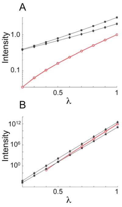
Increase of covariance peak intensity with respect to the exponent (λ) used in transforming the generalized covariance matrix. (A) Log-linear plot tracking the intensity build-up with increasing λ for three example traces from the simulated spectra of Figure 1. (B) Analogous plot for an experimental generalized indirect covariance (GIC) HMBC*TOCSY spectrum of a metabolite mixture. In panel B, the black curves belong to myo-inositol (stronger peak) and glucose (weaker peak). In all panels, black traces with filled circles correspond to expected signals while red traces with open circles correspond to false positive signals. Note the characteristically higher slopes of the false positive traces.

Materials and Methods

2D ¹H-¹H-TOCSY¹⁰ (90 ms mixing time using MLEV-17 ²⁴) and ¹³C-¹H-HMBC spectra¹⁷ were recorded at 18.8 T and 298 K for a mixture of seven common metabolites at natural ¹³C abundance (D-carnitine, D-glucose, L-glutamine, L-histidine, L-lysine, myo-inositol, and shikimic acid) each at a concentration of 10 mM in D₂O. The direct ¹H dimension of each spectrum was acquired with 2048 complex points and a spectral width of 8013 Hz. The indirect ¹H dimension of the TOCSY was acquired with 1024 complex points and the same spectral with as the direct dimension. The indirect ¹³C dimensions of the HMBC spectrum was acquired with 1024 complex points and a spectral width of 32206 Hz, respectively.

Additionally, 2D ¹H-¹H-TOCSY (50 ms mixing time using DIPSI-2 ²⁵) and ¹³C-¹H HMBC spectra were also recorded at 298 K using a sample of the MDM2-binding p53 peptide construct with sequence ETFSDLWKLLPEN, described previously.²⁶ The spectra were acquired with the same spectral widths as above but with half the number of complex points along each dimension, except for the indirect dimension of the TOCSY having only 256 complex points, and with a spectral width of 44643 Hz in the indirect (¹³C) dimension of the HMBC spectrum.

All spectra were recorded on a Bruker AVANCE 800 spectrometer equipped with a cryogenic probe and processed in NMRPipe.²⁷ For the HMBC spectra, a magnitude spectrum was calculated after 2D FT.¹⁷ All other calculations were performed in Matlab.²⁸

Results

To demonstrate the approach, a generalized indirect covariance (GIC) HMCB*TOCSY spectrum for a 2-component mixture was calculated from a simulated ¹³C-¹H HMBC spectrum (Fig. 1A) and ¹H-¹H TOCSY spectrum (Fig. 1B) with sharp lines. The mixture consists of two molecules represented by 2 different spin systems: the first has 3 linked ¹³C,¹H pairs X-Y-Z and the second has 2 pairs U-V. To simulate the effects of overlap, the protons of pairs Y and U are assigned degenerate chemical shifts. Related models with different degenerate chemical shifts were explored, but all gave results similar to those reported here. λ = 1 gives rise to a false peak in the generalized indirect covariance spectrum between C_X-H_V as indicated in (Fig. 1C).

Figure 1.

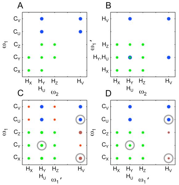
Schematic HMBC (A), TOCSY (B), [HMBC*TOCSY]¹ (C) and [HMBC*TOCSY]^0.5 (D) spectra for a model mixture containing one spin-system with 3 connected ¹³C-¹H pairs X-Y-Z and one spin-system consisting of 2 ¹³C-¹H pairs U-V where the carbon/carbon connectivities are between X-Y, Y-Z, and U-V. Note the degeneracy in chemical shift for the protons of ¹³C-¹H pairs Y and U, which leads to false positive (red) signals in the [HMBC*TOCSY]^λ=1 spectrum. Application of the matrix-square root in the GIC formalism eliminates most false positives. The two most intense false positives (dark red) are not completely suppressed with decreasing λ. They can be identified as false positives because of their large slope as a function of λ. The peaks circled in gray are those whose traces are displayed in Fig. 2.

Figure 2A shows the suppression of the false positive C_X-H_V peak (red) achieved by varying the exponent λ in Eq. (5). This log-linear plot demonstrates the higher slope (Eq. (8)) associated with the false positive signal (red) relative to the true signals (black).

Figure 2B shows the analogous plot for a GIC HMBC*TOCSY spectrum derived from experimental ¹³C-¹H-HMBC and ¹H-¹H TOCSY spectra of a metabolite mixture sample. The false positive signal, which incorrectly correlates a ¹³C resonance of myoinositol to a ¹H resonance of carnitine, exhibits a systematically stronger λ scaling compared to the true positive signals. Its intensity in the λ = 1 covariance matrix lies between the intensities of two true positive signals, a glucose cross-peak and a myoinositol cross-peak, but when λ = 0.5, its intensity is only as high as the weaker of the two true signals and the slope of its intensity build up as a function of λ is higher than the slope of the true signals. The higher slope and weaker intensity at λ = 0.5 provide a signature that this peak is a false positive.

Fig. 3 demonstrates the preferential suppression of artifact signals via the matrix-square root in two GIC HMBC*TOCSY covariance spectra calculated from two experimental pairs of ¹³C-¹H-HMBC and ¹H-¹H TOCSY spectra recorded of the metabolite mixture (Fig. 3A,B) and the p53 peptide (Fig. 3C,D). Peak intensity better separates false peaks (red dots) from true peaks (black dots) in the λ = 0.5 spectrum than in the λ = 1 spectrum (Fig. 3A,C and Table 1). However, while intensity in the λ = 1 spectrum alone is a relatively poor indicator of peak veracity, deviations from the trend visible amongst the true peaks in Fig. 3A,C are indicative of peak authenticity: peaks lying on the upper left hand side of the distribution marked by the ellipse, i.e. peaks for which the matrix-square root reduces peak intensity by a large amount, are most likely to be false.

Figure 3.

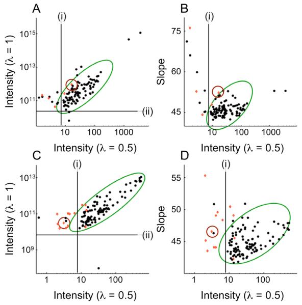
Suppression and identification of false positive signals via matrix-square root and λ scaling. (A,C) Comparison of intensity with λ = 1 and λ = 0.5 of (unsplit) peaks in covariance [HMBC*TOCSY]^λ spectra of (A) a metabolite mixture and (C) the p53-peptide. (B,D) Comparison of slope vs. intensity at λ = 0.5. Panels B and D show data corresponding to the pairs shown in panels A and C, respectively. Black dots represent data derived from true peaks while red dots belong to false peaks. Line (i) demarcates the minimum intensity for which peaks are picked in the λ = 0.5 spectrum, while line (ii) demarcates the minimum intensity for which peaks are picked in the λ = 1 spectrum. The green ellipses surround the bulk of data to guide the eye. The red circles enclose (A,B) the false positive peak shown in Figs. 2,4 and (C,D) the false positive peak shown in Fig. 5.

Table 1.

Reduction in False Positive Rate via Square-Root Extraction

	Metabolite mixture		p53 (MDM2 binding peptide)a
	λ = 1	λ = 0.5	λ = 1	λ = 0.5
True Peaks	107	103	103	101
False Peaks	6	2	15	4
False Positive Rate (%)	5	2	13	4

^aaliphatic/aliphatic ¹³C-¹H peaks

Plotting the slope (Eq. (8)) versus the intensity at λ = 0.5 also separates true from false peaks (Fig. 3B,D). Peaks characterized by especially high slopes relative to their intensity (above and to the left of the ellipse surrounding most peaks) are most likely to be false. In fact, plotting the slope versus the intensity at λ = 0.5 identifies false peaks more effectively than does plotting intensity at λ = 1 versus that at λ = 0.5.

The selection procedure can be formalized by applying principal component analysis (PCA) in two dimensions,²⁹ which in good approximation reproduces the ellipses drawn in Fig. 3. The major axis of the ellipse is given by the first principal component and the minor axis by the second principal component. PCA transforms intensity and slope into a new variable pair of independent statistics that is a linear combination of the original pair. The first principal component adjusts peak intensity using slope information, while the second component combines intensity and slope information into a measure of peak quality. Under the assumption that the principal components are Gaussian distributed, the value for the second principal component calculated for a given peak can be transformed into a p-value that quantifies the probability that this peak is real rather than an artifact arising from spurious chemical shift degeneracy.

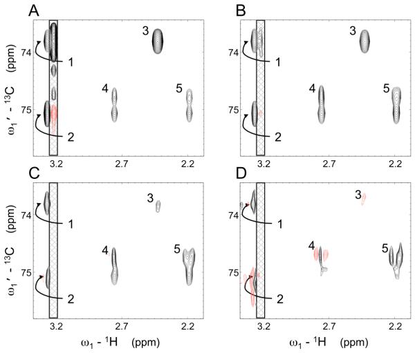
The following procedure allows one to edit peaks picked from a GIC derived spectrum: i) perform PCA as described above on (only) the peaks picked in the λ = 0.5 spectrum, ii) reject peaks for which the p-value calculated (as in a one-tailed test) from the second principal component is less than 5%. Application of this procedure cuts the false-positive rate (reported for the λ = 0.5 spectra in Table 1) in half while only rejecting one (p53 peptide) and two (metabolite mixture) true peaks. The peaks plotted in Fig. 3 include only those peaks reported in Table 1 whose line shapes do not qualitatively change as a function of λ as illustrated in Fig. 4. This figure shows a region of the metabolite mixture GIC [HMBC*TOCSY]^λ spectrum for different λ values. The unsymmetric covariance spectrum (λ = 1) displays a noise ridge (cross-hatched box) ¹⁶ due to the covariance of a signal arising from the carnitine methyl groups with noise. This ridge is suppressed after application of the matrix roots using the GIC formalism.

Figure 4.

Spectral region of [HMBC*TOCSY]^λ spectrum of a metabolite mixture with (A) λ = 1, (B) λ = 0.75, (C) λ = 0.5, (D) λ = 0.25. Black contours indicate positive signals, and red contours, negative signals. The cross-hatched region indicates a noise ridge, which is suppressed by the matrix power of λ ≤ 0.5. Decreasing the value of λ also effectively suppresses peak (3), an artifact due to chemical shift near-degeneracy (pseudo-relay) between myo-inositol and carnitine ¹H resonances. Peaks (1) and (2) arise from myo-inositol, while Peaks (4) and (5) arise from the geminal protons attached to C6 in the cyclohexene ring of shikimic acid. Their distorted line-shapes, particularly pronounced with λ = 0.25 (C,D) reflect J-splittings in the underlying HMBC and TOCSY spectra, corresponding to those observed in the 1D ¹H spectrum of shikimic acid available via the BMRB.³⁸

The decrease in intensity with decreasing λ for the false positive is again much more pronounced than for the other peaks: relative to the other peaks in panel A, peak (3) is quite strong whereas it is weak relative to the other peaks in panel C and negative in panel D. The slope given by Eq. (8) at λ = 0.5 for this peak is 52 while a slope of 45 is typical for this data set. This peak appears in the upper left of Fig. 3B (encircled in red) outside of the ellipse surrounding true peaks. Due to its high slope and low intensity at λ = 0.5, this peak can be easily identified and eliminated improving the analysis of the GIC HMBC*TOCSY spectrum.

Application of λ ≤ 0.5 also recovers the splitting present in the direct dimensions of the HMBC and TOCSY spectra of this mixture, which is lost by covariation of the direct dimension in the unsymmetric covariance process. However, the onset of distortions in line-shape (e.g. peak 2 in Fig. 3D) and signal reduction generally preclude the use of very low λ values (λ ≤ 0.25).

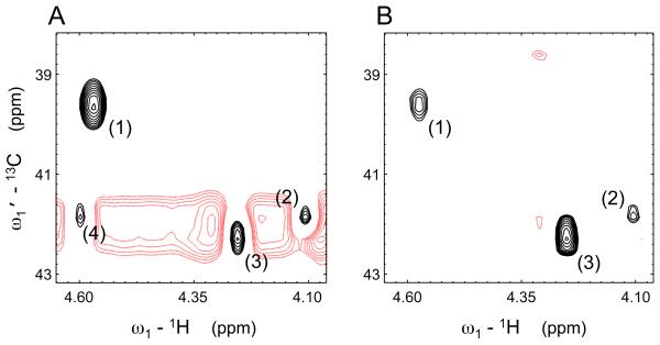
Fig. 5 shows a region of the GIC HMBC*TOCSY spectrum of the p53-peptide. Again, the matrix-square root suppresses a false positive peak and a ridge, demonstrating the applicability of generalized covariance to larger systems, such as peptides. Unlike an experimentally recorded HSQC-TOCSY, the GIC HMBC*TOCSY exhibits correlations connecting quaternary and other non-protonated carbons, such as carbonyl and carboxyl carbons as illustrated in Fig. 6. Thus, GIC provides a powerful representation of spectral information for the resonance assignment of small and large molecules, including peptides.

Figure 5.

Selected region of the generalized indirect covariance [HMBC*TOCSY]^λ spectrum of the p53 peptide calculated using (A) λ = 1 and (B) λ = 0.5. Black contours indicate positive signals, and red contours indicate negative signals. Peaks (1), (2) and (3) are Phe 3 (CB-HA), Lys 8 (CE-HA) and Leu 10 (CB-HA), respectively. Peak (4) is a pseudo-relay artifact caused by accidental near-degeneracy that is suppressed by the matrix-square root, which also eliminates the horizontal ridge in panel A.

Figure 6.

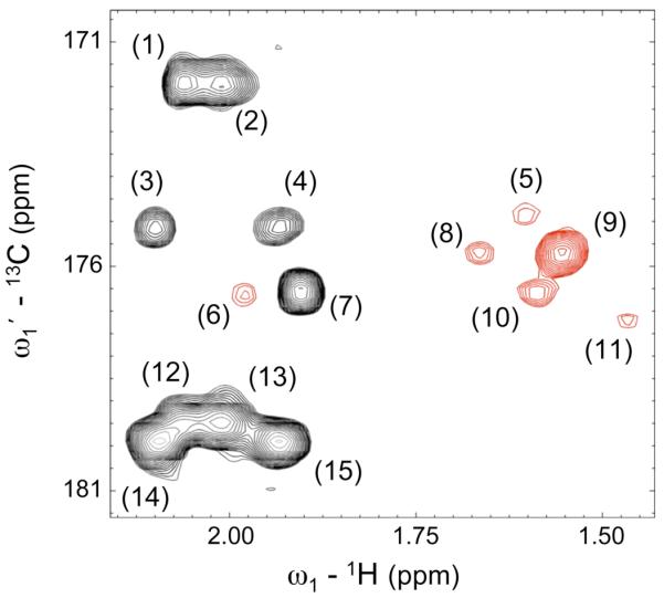
Novel long-range carbonyl-proton and carboxyl-proton correlations of p53 peptide derived from GIC [HMBC*TOCSY]^1/2. Cross-peaks initially present in the ¹³C-¹H-HMBC spectrum are depicted by black contours. Peaks arising from covariance of the HMBC with the ¹H-¹H TOCSY spectrum are colored in red. The assignments of the peaks are as follows: (1) Glu 12 (C’-HB2), (2) Glu 12 (C’-HB3), (3) Glu 1 (C’-HB2), (4) Glu 1 (C’-HB3), (5) Leu 9 (C’-HB2), (6) Pro 11 (C’-HG3), (7) Pro 11 (C’-HB3), (8) Lys 8 (C’-HB2), (9) Lys 8 (C’-HG2), (10) Leu 10 (C’-HG), (11) Leu 6 (C’-HG), (12) Glu 12 (CD-HB2), (13) Glu 12 (CD-HB3), (14) Glu 1 (CD-HB2) and (15) Glu 1 (CD-HB3). While ¹³C-¹H HSQC and HSQC-TOCSY spectra lack carbonyl/carboxyl-proton cross-peaks, the ¹³C-¹H HMBC spectrum correlates carbonyl and side-chain carboxyl carbons (such as the δ-carbons of glutamic acid) with protons via 2 and 3 bond correlations. The inclusion of TOCSY information via GIC processing results in longer-range correlations such as those shown here in red.

Discussion and Conclusions

Many informative spin correlations are not directly accessible by experiment by multidimensional NMR due to measurement and sensitivity considerations. For instance, correlations between insensitive nuclei can often be observed only indirectly, i.e. via correlations between those nuclei via protons. Other spectra, such as heteronuclear NOESY and TOCSY, which contain useful information for resonance assignment and structure determination of complex molecules, are often not collected due to limited sensitivity and spectrometer time constraints. However, unsymmetric covariance NMR can reconstruct heteronuclear TOCSY and NOESY spectra from homonuclear NOESY and TOCSY spectra and common heteronuclear ¹³C-¹H HSQC or HMBC spectra.⁷

Similarly, the high-dimensional correlation information required to make chemical shift assignments in polypeptides can often only be practically measured by a series of lower dimensional spectra. A typical manual analysis of NMR spectra establishes higher order correlations via a comparison of strip plots. Visual assessment of a non-vanishing correlation of peaks between slices (strip plots) in two NMR spectra links the spin-systems associated with the strip plots being compared. Automated analysis methods, particularly those for protein backbone assignment,^30-37 often work with peak lists rather than with the underlying spectra. However, such methods generally require high quality peak lists that are manually curated. Recently developed methods such as hyperdimensional NMR,^11,12 COBRA¹³ and Burrow-Owl¹⁵ use unsymmetric covariance^5,7 to automate the traditional manual approach of establishing spin correlations via comparison of strip plots, prior to peak picking. However, the application of such methods can confound downstream analysis due to the presence of spurious correlations between strip plots caused by (near-)degenerate chemical shifts and therefore may benefit from the generalized indirect covariance approach presented here. GIC establishes correlations between spectra rather than peak lists and thereby ‘delays’ the otherwise iterative and sometimes difficult process of peak picking until true peaks become self-evident.

The GIC formalism generalizes the use of the matrix-square root for the suppression of relay effects and pseudo-relay effects, originally demonstrated for symmetric covariance NMR spectra,^18,19 to unsymmetric covariance spectra.⁶ Previous work in covariance reconstruction of unsymmetric spectra compared unsymmetric and indirect covariance results in order to identify artifacts in each.²⁰ The generalized covariance matrix (Eq. (3)) presented here computes both unsymmetric and symmetric covariance spectra in the same step. Furthermore, the GIC formalism allows for the extraction of multiple roots in a single covariance calculation. For the examples used here, extraction of the square root via the generalized covariance matrix reduces the false positive count of a HMBC*TOCSY spectrum by about a factor of three. Removal of peaks characterized by weak intensity following extraction of the square root concomitant with a rapid intensity build up with λ further reduces the false positive rate.

The generalized covariance formalism addresses the issue of false positives in unsymmetric covariance spectra caused by resonance overlap and extends the applicability of unsymmetric covariance NMR to systems with an increased number of signals of greater resonance degeneracy, including complex mixtures, for example of metabolites, and biological macromolecules, such as peptides and proteins. By providing a mechanism to identify false positive correlations, generalized indirect covariance lays a linear-algebraic foundation for the accurate and sensitive identification of spin correlations that are distributed over multiple 2D NMR spectra. The establishment of spin correlations that are not easily experimentally observable via an automated method analogous to the comparison of strip plots, mark a path toward the development of computer-based assignment procedures that are as robust as are the most expert manual analyses of NMR data.

Abbreviations

NMR

Nuclear Magnetic Resonance

SVD

Singular Value Decomposition

References

- 1.Ernst R, Bodenhausen G, Wokaun A. Principles of Nuclear Magnetic Resonance in One and Two Dimensions. Clarendon Press; Oxford: 1987. [Google Scholar]
- 2.Jaravine V, Ibraghimov I, Orekhov VY. Nature Methods. 2006;3:605–607. doi: 10.1038/nmeth900. [DOI] [PubMed] [Google Scholar]
- 3.Friebolin H. Basic One- and Two-Dimensional NMR Spectroscopy. Wiley-VCH; Weinheim: 2005. [Google Scholar]
- 4.Zhang F, Brüschweiler R. J. Am. Chem. Soc. 2004;126:13180–13181. doi: 10.1021/ja047241h. [DOI] [PubMed] [Google Scholar]
- 5.Blinov KA, Larin NI, Kvasha MP, Moser A, Williams AJ, Martin GE. Magn Reson Chem. 2005;43:999–1007. doi: 10.1002/mrc.1674. [DOI] [PubMed] [Google Scholar]
- 6.Blinov KA, Larin NI, Williams AJ, Mills KA, Martin GE. J. of Heterocycl. Chem. 2006;43:163–166. [Google Scholar]
- 7.Blinov KA, Larin NI, Williams AJ, Zell M, Martin GE. Magn Reson Chem. 2006;44:107–109. doi: 10.1002/mrc.1766. [DOI] [PubMed] [Google Scholar]
- 8.Blinov KA, Williams AJ, Hilton BD, Irish PA, Martin GE. Magn Reson Chem. 2007;45:544–546. doi: 10.1002/mrc.1998. [DOI] [PubMed] [Google Scholar]
- 9.Bodenhausen G, Ruben DG. Chem. Phys. Lett. 1980;69:185–189. [Google Scholar]
- 10.Braunschweiler L, Ernst RR. J. Magn. Reson. 1983;53:521–528. [Google Scholar]
- 11.Kupce E, Freeman R. J. Am. Chem. Soc. 2006;128:6020–6021. doi: 10.1021/ja0609598. [DOI] [PubMed] [Google Scholar]
- 12.Kupce E, Freeman R. Progr. Nucl. Magn. Reson. Spectr. 2008;52:22–30. [Google Scholar]
- 13.Lescop E, Brutscher B. J. Am. Chem. Soc. 2007;129:11916–11917. doi: 10.1021/ja0751577. [DOI] [PubMed] [Google Scholar]
- 14.Lescop E, Rasia R, Brutscher B. J. Am. Chem. Soc. 2008;130:5014–5015. doi: 10.1021/ja800914h. [DOI] [PubMed] [Google Scholar]
- 15.Benison G, Berkholz DS, Barbar E. Journal of Magnetic Resonance. 2007;189:173–181. doi: 10.1016/j.jmr.2007.09.009. [DOI] [PubMed] [Google Scholar]
- 16.Snyder DA, Ghosh A, Zhang F, Szyperski T, Brüschweiler R. J. Chem. Phys. 2008;129:104511. doi: 10.1063/1.2975206. [DOI] [PMC free article] [PubMed] [Google Scholar]
- 17.Bax A, Summers MF. J. Am. Chem. Soc. 1986;108:2093–2094. [Google Scholar]
- 18.Brüschweiler R. J. Chem. Phys. 2004;121:409–414. doi: 10.1063/1.1755652. [DOI] [PubMed] [Google Scholar]
- 19.Trbovic N, Smirnov S, Zhang FL, Brüschweiler R. Journal of Magnetic Resonance. 2004;171:277–283. doi: 10.1016/j.jmr.2004.08.007. [DOI] [PubMed] [Google Scholar]
- 20.Martin GE, Hilton BD, Blinov KA, Williams AJ. Magn Reson Chem. 2008;46:138–43. doi: 10.1002/mrc.2141. [DOI] [PubMed] [Google Scholar]
- 21.Macura S, Ernst RR. Molecular Physics. 1980;41:95–117. [Google Scholar]
- 22.Snyder DA, Zhang F, Brüschweiler R. J. Biomol. NMR. 2007;39:165–175. doi: 10.1007/s10858-007-9187-1. [DOI] [PubMed] [Google Scholar]
- 23.Kupce E, Freeman R. Magn Reson Chem. 2007;45:103–105. doi: 10.1002/mrc.1947. [DOI] [PubMed] [Google Scholar]
- 24.Bax A, Davis DG. J. Magn. Reson. 1985;65:355–360. [Google Scholar]
- 25.Shaka A, Lee C, Pines A. J. Magn. Reson. 1988;77:274–293. [Google Scholar]
- 26.Showalter SA, Bruschweiler-Li L, Johnson E, Zhang F, Brüschweiler R. J. Am. Chem. Soc. 2008;130:6472–6478. doi: 10.1021/ja800201j. [DOI] [PubMed] [Google Scholar]
- 27.Delaglio F, Grzesiek S, Vuister GW, Zhu G, Pfeifer J, Bax A. J. Biomol. NMR. 1995;6:277–93. doi: 10.1007/BF00197809. [DOI] [PubMed] [Google Scholar]
- 28.The Mathworks Inc. 7.1.0.183 ed 2005.
- 29.Jolliffe IT. Principal Component Analysis. 2nd ed Springer; New York: 2002. [Google Scholar]
- 30.Altieri AS, Byrd RA. Curr. Opin. Struct. Biol. 2004;14:547–553. doi: 10.1016/j.sbi.2004.09.003. [DOI] [PubMed] [Google Scholar]
- 31.Moseley HNB, Monleon D, Montelione GT. Nuclear Magnetic Resonance of Biological Macromolecules, Pt B. 2001;339:91–108. doi: 10.1016/s0076-6879(01)39311-4. [DOI] [PubMed] [Google Scholar]
- 32.Li KB, Sanctuary BC. J. Chemical Information and Computer Sciences. 1997;37:359–366. doi: 10.1021/ci960372k. [DOI] [PubMed] [Google Scholar]
- 33.Xu YZ, Wang XX, Yang J, Vaynberg J, Qin J. J. Biomol. NMR. 2006;34:41–56. doi: 10.1007/s10858-005-5358-0. [DOI] [PubMed] [Google Scholar]
- 34.Wang JY, Wang TZ, Zuiderweg ERP, Crippen GM. J. Biomol. NMR. 2005;33:261–279. doi: 10.1007/s10858-005-4079-8. [DOI] [PubMed] [Google Scholar]
- 35.Jung YS, Zweckstetter M. J. Biomol. NMR. 2004;30:11–23. doi: 10.1023/B:JNMR.0000042954.99056.ad. [DOI] [PubMed] [Google Scholar]
- 36.Coggins BE, Zhou P. J. Biomol. NMR. 2003;26:93–111. doi: 10.1023/a:1023589029301. [DOI] [PubMed] [Google Scholar]
- 37.Atreya HS, Sahu SC, Chary KVR, Govil G. J. Biomol. NMR. 2000;17:125–136. doi: 10.1023/a:1008315111278. [DOI] [PubMed] [Google Scholar]
- 38.Ulrich EL, Akutsu H, Doreleijers JF, Harano Y, Ioannidis YE, Lin J, Livny M, Mading S, Maziuk D, Miller Z, Nakatani E, Schulte CF, Tolmie DE, Wenger RK, Yao HY, Markley JL. Nucl. Acids. Res. 2008;36:D402–D408. doi: 10.1093/nar/gkm957. [DOI] [PMC free article] [PubMed] [Google Scholar]