Fast Detection of the Optic Disc and Fovea in Color Fundus Photographs

Abstract

A fully automated, fast method to detect the fovea and the optic disc in digital color photographs of the retina is presented. The method makes few assumptions about the location of both structures in the image. We define the problem of localizing structures in a retinal image as a regression problem. A kNN regressor is utilized to predict the distance in pixels in the image to the object of interest at any given location in the image based on a set of features measured at that location. The method combines cues measured directly in the image with cues derived from a segmentation of the retinal vasculature. A distance prediction is made for a limited number of image locations and the point with the lowest predicted distance to the optic disc is selected as the optic disc center. Based on this location the search area for the fovea is defined. The location with the lowest predicted distance to the fovea within the foveal search area is selected as the fovea location. The method is trained with 500 images for which the optic disc and fovea locations are known. An extensive evaluation was done on 500 images from a diabetic retinopathy screening program and 100 specially selected images containing gross abnormalities. The method found the optic disc in 99.4% and the fovea in 96.8% of regular screening images and for the images with abnormalities these numbers were 93.0% and 89.0% respectively.

1 Introduction

Detection of the optic disc and fovea location in retinal images is an important aspect of the automated detection of retinal disease in digital color photographs of the retina. Together with the vasculature, the optic disc and the fovea are the most important anatomical landmarks on the posterior pole of the retina. The optic disc is the area of the retina where the retinal vasculature enters and leaves the eye and it marks the exit point of the optic nerve. The appearance of the optic disc is different from the surrounding retinal tissue (see Figure 1) and parts of the disc can potentially be classified as abnormal by disease detection algorithms, detecting and masking the disc is the main motivation for this work. Examples of abnormalities that can be confounded with the optic disc are exudates, cottonwool spots and drusen [1]. Additionally, the optic disc location is useful in the automated tracking of glaucoma [2] and the detection of neovascularisations on the optic disc, a rare but serious abnormality. The fovea is responsible for sharp central vision and is located in the center of a darker area (see Figure 1). Because of its important function in vision, the distance at which lesions are located from the fovea influences their clinical relevance [3].

Fig. 1.

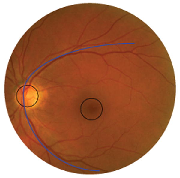
A digital color fundus photograph with a circle marking the optic disc (left) and another circle in the center of which is the fovea. The vascular arch marked in the image is formed by the major arteries and veins that leave the optic disc up- and downwards.

This work is part of a larger project to develop an automated screening system for diabetic retinopathy. Diabetic retinopathy is a common complication of diabetes and the largest cause of blindness and vision loss in the working population of the western world [4]. We have previously published the results of large scale evaluations of a comprehensive automated screening system on 10,000 exams (40,000 images) [5] and 15,000 exams (60,000 images) [6]. Analysis of the results of these evaluations indicated that the location of the optic disc and especially location of the fovea may potentially be useful in improving the detection of subtle cases of diabetic retinopathy. A number of exams missed by the automated screening system contained only one or two lesions, however, these were located close to the fovea and were thus marked as “suspect” by the screening program ophthalmologists. It is our expectation that information about the location of lesions on the retina may help the system to detect these cases.

A substantial number of publications have dealt with the detection of the location of just the optic disc (see [7] for an overview). The state-of-the-art optic disc localization methods use the orientation of the vasculature to detect the position of the optic disc [7–11]. Detection of the fovea has received less attention, likely due to the fact the fovea is harder to detect and does not feature any high contrast structures. Sinthanayothin et al. [12] used the increased pigmentation around the fovea to detect its location using a template matching technique and reported a performance of 80.4% on 100 images. Li et al. [13] used a similar cue to find the fovea and additionally used the location of the vascular arch (see Figure 1) to constrain the search area. A detection performance of 100% for the fovea is reported on 89 images.

Recently, we have presented an automated method [10] to detect the location of the optic disc and fovea. The method used an optimization method to fit a point distribution model [14] to the fundus image. After fitting, the points of the model indicated the location of the normal anatomy. This method was able to find the fovea location in 94.4% and the optic disc in 98.4% of 500 images. On a separate set of 100 heavily pathological images the system showed a performance of 92.0% and 94.0% respectively. The method requires the vascular arch to be at least partially visible but works on images centered on the fovea as well as centered on the optic disc. Tobin et al. [9] presented an automatic method for detection of the optic disc and the fovea. The method started by locating the optic disc and the vascular arch. Based on these two anatomical landmarks the location of the fovea was inferred. The authors reported 90.4% detection performance for the optic disc and 92.5% localization performance for the fovea in 345 images. The method requires that retinal images are approximately centered on the fovea and that the vascular arch is visible. A similar method for fovea centered images was presented by Fleming et al. [11]: after detection of the vascular arch the optic disc is found using a Hough transform and the fovea is detected by template matching where the template was derived from a set of training images. The optic disc was detected in 98.4% of cases and the fovea in 96.5% of cases in 1056 images.

The main issue with the previous methods that use the vascular arch is that they require it to be visible in the image and most methods are developed for fovea centered images only. The screening data in typical screening programs is acquired at different sites, using different cameras and operators. This leads to a substantial variability in the image quality as well as imperfect adherence to the imaging protocol. The screening protocol used by the particular screening program [15] that provides the images used in this work requires the acquisition of two images per eye, one centered on the optic disc and one centered on the fovea. Half of the screening images in the program that supplied the data used in this study are therefore optic disc centered. Methods that require the visibility of the complete vascular arch generally make strong assumptions about the way in which an image is acquired and are less well suited for application on the real world screening data. Screening programs can be structured in different ways. In case of an on-line system where the patient receives almost immediate feedback, rapid processing of the image data is key. In a program where the images are processed off-line, speed may be less of an issue but due to the scale of population screening programs (e.g. hundreds of thousands of patients) an in increase in processing speed will have a large impact on the overall efficiency and throughput. Our own previously presented system [10] uses a complex optimization procedure and will take approximately 10 minutes to find the anatomical landmarks. The method by Fleming et al. [11] takes 2 minutes to process an image. Tobin et al. [9] did not report the processing time of their algorithm. As these algorithms were not all benchmarked on the same computer system, the runtime should only be used as an indication and not to directly compare the different methods.

We propose to formulate the problem of finding a certain position in a retinal image as a regression problem. A kNN regressor is trained to estimate the distance to a certain location in a retinal image (i.e. the optic disc and the fovea) given a set of measurements obtained around a circular template placed at a certain location in the image. By finding the position in the image where the estimated distance is smallest, both the optic disc and fovea can be detected.

The main contribution of this work is a fast, robust method for the detection of the location of the optic disc and the fovea. The method makes few assumptions about the way in which the retinal image has been acquired (i.e. optic disc centered or fovea centered) but does require the larger part of the optic disc and the fovea to be in the image in order to successfully detect their location. The method integrates cues from both the local vasculature and the local image intensities. The method is trained using 500 images and is evaluated on a separate, large dataset of 600 images.

This paper is structured as follows. Section 2 describes the data used in this research. The method itself is described in Section 3. The results of the algorithm are shown in Section 4. The paper end with a discussion and conclusion in Section 5.

2 Materials

In this work 1100 digital color fundus photographs were used. They were sequentially selected from a diabetic retinopathy screening program [15]. The images represent real world screening data, acquired at twenty different sites using different cameras at different resolutions. In all cases JPEG image compression was applied. Each of the images was acquired according to a screening imaging protocol. From each eye two digital color photographs were obtained, one approximately centered on the optic disc and one approximately centered on the fovea. Three different camera types were used; the Topcon NW 100, the Topcon NW 200 and the Canon CR5-45NM.

1000 of the 1100 images were randomly selected from our source screening image set of 40,000 images to represent typical screening data. The characteristics of the randomly selected image data is shown in Table 1. Typical screening data does not contain much serious pathology and the presence of heavy pathology makes detecting the optic disc and fovea more difficult. Therefore, an additional set of 100 images were selected, using our automated screening system [6], to represent the most pathological images in the source screening set. The following types of abnormalities were present in this set of images: microaneurysms (59%), hemorrhages (72%), exudates (50%), cottonwool spots (29%) and neovasculariza-tions (6%). Other abnormalities found in the set are: drusen (14%), scarring (10%) and preretinal hemorrhage (1%). Fourteen images with laser treatment scarring were also included, as laser treatment severely disturbs the background appearance of the retina. Acceptable quality, as judged by the screening program ophthalmologists, was a selection criterion in all cases. The screening ophthalmologists find the quality acceptable if it does not prevent them from assessing the presence of diabetic retinopathy. The set of 1000 typical screening images was split into a training set of 500 images and a test set of 500 images. A single human observer segmented all images. To enable comparison with the automated method a second observer segmented the 500 images in the test set as well as the 100 images in the pathological set. Both human observers were medical students who received training in the analysis of retinal images. Observers marked the optic disc center and four points on the optic disc border as well as a single point in the center of the fovea location. The four points on the optic disc border were used to determine a rough segmentation of the optic disc. By interpreting the distance of each of the four points to the optic disc center point as local optic disc radii, the optic disc radius at any angle can be estimated using linear interpolation which allows us to generate a rough segmentation of the complete optic disc from the four marked border points.

Table 1. The characteristics of the set of images used in this research.

Characteristics of the Image Set
Number of Images	Size (pixels)	Coverage
597	768 × 576	45
368	1792 × 1184	45
114	2048 × 1536	45
9	2160 × 1440	45
7	1536 × 1024	35
3	1280 × 960	45
2	768 × 576	35

3 Methods

3.1 Pre-processing

Each of the images is pre-processed before the localization of the optic disc and the fovea commences. First the FOV is detected by calculating the gradient magnitude of the red plane of the image. Several different FOV masks are then fitted to this gradient magnitude image and the best fitting mask is chosen. The template-masks have been previously manually segmented, when a new camera is added to the screening program pool its FOV mask image is segmented and stored. This template based method is used because some of the images are locally underexposed, a common issue in non-mydriatic images, which would result in holes in the FOV segmentation when just using a threshold to segment the FOV. Since there is a wide variety in image sizes each image is scaled so that the width of its FOV is 630 pixels. The FOV width is not a critical parameter and the described detection method will work with any size FOV as long as all images are resized in the same way. Choosing a smaller size FOV does have positive effect on the computational complexity. Do note that the resizing does not account for differences in the number of degrees of the retina covered by the FOV. This is because the amount of coverage is not stored with the images and as such unknown to us. We attempt to compensate for this in the method by choosing the foveal search area relatively large. The large gradient at the edge of the FOV can disturb feature extraction close to the border of the FOV. To remove it, a mirroring operation is carried out in which the pixel values inside the FOV are copied to the area outside the FOV as follows. For each pixel position o outside the FOV a line is projected to the closest point b on the border of the FOV at distance d from o. From b the line is then extended into the FOV and the pixel value at distance d from b is then copied to o.

The presented optic disc and fovea localization method uses only the green plane of the color image. To remove any low frequency gradients over the image, the green plane of the image is blurred using a Gaussian filter with a large variance, i.e. σ = 70 pixels, and this blurred image is subtracted from the original. The size of σ is not a critical parameter but should be sufficiently large so that no retinal structures are visible in the blurred image. The most important prerequisite of the method is the availability of a vessel segmentation. We have used a pixel classification based method [16]. In this approach a kNN classifier is trained using example pixels that have been labeled as either vessel or non-vessel. We used the 20, hand labeled training images from the DRIVE database [17] for this purpose. A Gaussian filterbank that contains Gaussian derivatives up to and including second order at five different variances (i.e. σ = 1, 2, 4, 8,16) provides the features for each of the pixels. The trained kNN classifier assigns each pixel in the image a posterior probability p with p ∈ [0 … 1] that that pixel is inside a vessel based on the filterbank outputs. The posterior probability is given by $p=\frac{v}{k}$ where v is the number of training samples that are vessel amongst the k nearest neighbors in the feature space of the pixel under consideration.

3.2 Position Regression

We propose to define the problem of locating anatomical structures in retina images as a regression problem. In regression, an empirical function is derived from a set of experimental data [18]. In general, regression analysis considers pairs of measurements (d,x) where variable x represents a set of measurements, the independent variables. The goal of regression is to find a function f(•) that can be used to predict the dependent variable d from x.

$$d=f(\text{x},\text{p})+\epsilon$$ (1)

Here p is a parameter vector that controls the behavior of f(•) and ε is the error in the prediction of d by f(•). Naturally one would like to choose parameter vector p so as to minimize ε. The problem of finding a certain location l in an image can be formulated as a regression problem [19] by taking the distance in the image to l as the dependent variable d and taking an image derived measurement as the independent variable x. The regression function can then be determined using a set of examples for which the distance to l, d as well as x are known. To find l in a new image, one only needs to find the location in which the estimated distance to l in that image is minimal. We propose to use a k-Nearest Neighbor (kNN) regressor [20] as it performed well in preliminary experiments and allows straightforward feature selection. The regression function f(•), in this case parameter vector p only contains a single parameter, k, the number of neighbors. The kNN regressor requires a training phase in which measurement pairs (d, x) that are collected from various locations in a set of training images are put together in a training set. The measurement vectors in the training set x span a higher dimensional space, the feature space [21]. The estimated value of the dependent variable, d̂, for an independent variable y measured somewhere in an image is determined by the values of d associated with the k nearest neighbors in the feature space of y in the training set. By taking the average value of d amongst the k nearest neighbors d̂ is determined.

3.3 Vessel Analysis

The local orientation and width of the retinal vasculature provide important clues to the position on the retina. After pre-processing a posterior probability vessel map is available. To obtain a binary vessel map a threshold should be applied. Selection of the threshold is not critical and, for our vessel segmentation algorithm, independent of the used image database. It should be chosen low enough to include some of the smaller vessels around the fovea in the binary vessel map, we set it to 0.4. The binary map is thinned [22,23] until only the centerlines of the vessels remain. All cross-over points and bifurcations are eliminated by removing those centerline pixels that have more than two neighbors. This is necessary because vessel orientation is not well defined in these points. The orientation of the vessels is measured for each vessel centerline pixel by applying principal component analysis on its coordinates and those of its neighboring centerline pixels to both sides. The direction of the largest eigenvector of the covariance matrix of the set of 2D points, the first principal component, indicates the orientation of the vessel around the centerline pixel under consideration. In this work three pixels to both sides were used to determine the orientation. This is not a critical parameter, it was determined that this value gave adequate results in preliminary experiments. Those pixels near to the end of a segment that do not have three pixels to both sides use only the available pixels to determine the orientation. As it is not known in which direction the vessel flows, the local orientation α is expressed in radians where α ∈ [0…π].

The local vessel width w is measured for each centerline pixel on a line perpendicular to α. The distance from the centerline at which the posterior probability drops below half of the posterior probability value under the centerline pixel is selected as the vessel edge. After the distance to the left and right edge of the vessel has been determined their sum is taken as the local vessel width. The ends of vessel segments can be near bifurcation points or vessel crossings and these can distort the vessel width measurements leading to a width overestimation. To compensate for this effect we replace the width measurements in the last 3 pixels on both sides of each segment with the average of the width of their neighboring 3 pixels. In case a vessel segment is too short, less pixels are used. The absolute vessel width is dependent on the number of degrees covered by the FOV and varies between subjects and in time due to the cardiac cycle. Therefore the measured w are normalized by dividing them by the maximum measured w in the image.

3.4 Template Based Feature Extraction

There are many different independent variables (i.e. features) that can be measured in a retinal image and that may give information about the location in the image where one is measuring them. From the literature (see [7] for an overview) two important cues that determine the location in the image emerge, image intensity based cues and vasculature based cues. For both the optic disc and the fovea, image intensity can be an important cue due to the fact that the optic disc in general is brighter than the surrounding retinal tissue and the fovea tends to be in a darker, more pigmented area of the retina. In this work, all image intensity based measurements are obtained in the green plane of the RGB retinal image. The pattern of the vasculature as it flows from and to the optic disc over the retina is similar in all images and the width of the vasculature changes as one moves further away from the optic disc. As such the local orientation and width of vessels provide important cues about the location in the image.

As both the optic disc and fovea are essentially circular objects we propose to define a set of features measured under and around two circular templates. Figure 2 shows both the optic disc and fovea templates. The main difference between the two templates is the presence of an inner and outer section in the fovea template. This difference is to enable the template to measure intensity differences between the inner and outer parts of the template. The fovea is a “blob-like” structure with a lower intensity near its center and a progressively increasing intensity as one moves away from the center. Both templates consist of four quadrants and for each quadrant a set of features will be measured independently. The subdivision leads to more sensible features because one expects the vessels around the optic disc and the fovea to have a specific orientation at the border of each of the four quadrants when the templates are placed on the optic disc and fovea in a retinal image. Figure 1 shows the outlines of both the templates at their correct positions in a retinal image. Both of the templates have a radius, r_OD and r_fovea, which are free parameters that are dependent on the size of the image as well as the number of degrees of the retina shown in the FOV. The radius of the inner section of the fovea template is defined as $\frac{2}{3}{r}_{\text{fovea}}$. As the number of degrees imaged in the FOV is unknown we performed some preliminary experiments and set r_OD = r_fovea = 40 pixels, roughly the radius of the objects of interest in our training set after pre-processing. The circles in Figure 1 show the size of the template with respect to the size of the image.

Fig. 2.

a) The template used to extract features for localization of the optic disc. b) The template used to extract feature for localization of the fovea.

The templates can now be used to extract features at a particular (x, y) location in the image. The template is centered on the location under consideration (see Figure 3 for an example) and the following set of features are measured for both the optic disc and fovea template:

Fig. 3.

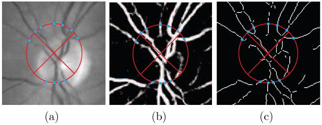
The optic disc template placed in a fundus image and two derived images. The points where unique vessel segments cross the template border are indicated by the blue dots. a) The green plane of the color fundus photograph. b) The vessel probability map. c) The skeletonized vessel segmentation. The vessel centerline points that lie on the template border, marked by the dots, are the locations where the local vessel width and orientation based features are measured.

1. Number of vessels. A count of the number of unique vessel segments intersecting the template border.

2. Average width of the vessels. The average value of w associated with the centerline pixels on the template border of the unique vessel segments from feature 1.

3. Standard deviation of the vessel width. The standard deviation of the measurements acquired in feature 2.

4. Average difference in orientation with either the x (quadrant I and III) or y-axis (quadrant II and IV). The orientation difference for quadrants I and III was defined as the |cos(α)| while for quadrant II and IV it was defined as sin(α).

5. Standard deviation of the orientation difference. The standard deviation of the measurements acquired in feature 4.

6. Maximum vessel width. Maximum value of w measured when calculating feature 2.

7. Orientation of the vessel with the maximum width. The value of α for the vessel segment with maximum w encountered while calculating feature 2.

8. Density of the vessels under the template. The total number of pixels under the template divided by the number of pixels marked as vessel in the binary vessel map.

9. Average vessel width under the complete template. The number of pixels under the template marked as vessel in the binary vessel map divided by the number centerline pixels under the template. This is a different way of measuring this than using the widths as determined at every centerline pixel.

   The following features (10 and 11 of the optic disc template) are only calculated for the optic disc template:

10. Average image intensity under the complete template. The average of all pixel intensities of the pixels in the pre-processed green plane of the retinal image that are under the template.

11. Standard deviation of the image intensity under the complete template. The standard deviation of the measurements acquired in feature 10.

    The following features (10 to 13 of the fovea template) are only calculated for the fovea template:

12. (10) Average image intensity under the outer template. The average of all pixel intensities of the pixels in the pre-processed green plane of the retinal image that are under the outer part of the fovea template.

13. (11) Standard deviation of the image intensity under the outer template. Standard deviation of the measurements acquired for feature 10.

14. (12) Average image intensity under the inner template. Same as feature 10 but under the inner part of the fovea template.

15. (13) Standard deviation of the image intensity under the inner template. Same as feature 11 but only under the inner part of the fovea template.

Features 1-7 are calculated independently for each quadrant bringing the total number of extracted features for the optic disc template to 7 × 4 + 4 = 32 and for the fovea template to 7 × 4 + 6 = 34. In case a feature cannot be measured, e.g. because the template is partially outside the field of view or there are no vessels under the template, the feature values are set to 0.

The cues listed earlier in this Section form the inspiration for the choice of this initial featureset. Features 1-9 attempt to characterize the local vessel pattern that is clearly different when the template is positioned on the optic disc as opposed to when it is positioned on the fovea. At the optic disc location one expects a large number (i.e. high density) of both very wide (i.e. the widest in the image) and narrow vessels that are flowing in a distinct direction which is different for every quadrant. The optic disc specific intensity features 10 and 11 simply characterize the local image intensity and standard deviation which are both expected to have a high value on top of the optic disc due to the bright appearance of the nerve tissue combined with the low intensity of the vessels. For the fovea template specific features 10-13 characterize the intensity and it's standard deviation in the central part of the template and in a ring around it. This should allow the system to determine if the template is centered on a “blob-like” structure such as the fovea.

3.5 Training Phase

3.5.1 Extraction of Training Samples

Before a regressor can be used to find a location in a previously unseen image, a one-time training phase needs to be completed. The training phase consists of the extraction of measurement pairs from a set of training images. To extract the measurement pairs from the 500 training images a two step sampling process was employed. In the first step the area around the known, correct object of interest within the radius of the template, r, was sampled in a uniform grid spaced 8 pixels apart resulting in about 78 measurements per image. The spacing of the grid is not an important parameter as long as this area is sampled densely enough. For each of the sampled locations the appropriate template was used to extract all features which were stored in the training sample set together with the distance d to the true center of the object of interest. It is unlikely that the features measured around the template can provide accurate information for a robust estimation of d further away from the object of interest. Therefore, all samples obtained further than r away from the object of interest were assigned the value d = r. In a second step a substantial number (500) of randomly selected locations (i.e. not on a grid) in the training image were sampled in a similar fashion.

3.5.2 Selection of k

Both k and the feature set have an influence on the regression performance. However, without assigning a value to k the wrapper based feature selection procedure can not be performed. Therefore, the regressor parameter k is first determined on the training data using the complete set of features. To accomplish this, the training image set was randomly split into two sets of 250 images. For each of the images in both sets the procedure as outlined above was applied and this meant that for both sets 144,500 measurement pairs were extracted into two sample sets. All the extracted features were normalized to zero mean and unit standard deviation. The value of parameter k was varied between 1 and 199 in steps of 2. For each value of k the average prediction error given by

$$\overline{\epsilon }=\frac{1}{N}\sum _{i=1}^N\left|d-\widehat{d}\right|$$ (2)

over the N measurement pairs in the second half of the training sample set was determined and the value that minimized ε̄ was chosen (see Figure 4). For the optic disc template this was k = 21 and for the fovea template this was k = 13.

Fig. 4.

A graph plotting the average prediction error ε̄ in pixels against the k parameter value of the kNN regressor in part of the training set.

3.5.3 Regression Feature Selection

A relatively large set of features has been defined. This complete set of features does not necessarily provide the best regression results. Application of a feature selection method may improve overall system performance and will decrease the computational complexity by reducing the dimensionality of the feature space. We have applied a supervised wrapper based feature selection method, Sequential Floating Feature Selection (SFFS) [24]. The algorithm adds and removes features to and from the selected feature set when that improves the performance of the regressor. The performance in this case is measured by the average ε, the prediction error, over the dataset. This feature selection technique was applied separately to both the optic disc and the fovea training set.

To perform the feature selection the training set was randomly split into two sets of 250 images (144,500 measurements pairs), the same sets that were used for determination of the optimal value of k. All the extracted features were normalized to zero mean and unit standard deviation. The SFFS algorithm would train the kNN regressor on the first set and then determine dˆ for each of the measurement pairs in the second set for different combinations of features. The set of features that minimized Equation 2 for the N measurement pairs in the second set was selected as the final set of features. For the optic disc template 16 features were chosen in the following order (more important to less important):

1. Average image intensity under the complete template.

2. Density of the vessels under the template.

3. Number of vessels (quadrant IV).

4. Number of vessels (quadrant I).

5. Average difference in orientation (quadrant III).

6. Average difference in orientation (quadrant I).

7. Standard deviation of the image intensity under the complete template.

8. Average width of the vessels (quadrant III).

9. Average width of the vessels (quadrant I).

10. Average width of the vessels (quadrant II).

11. Orientation of the vessel with the maximum width (quadrant III).

12. Average width of the vessels (quadrant IV).

13. Orientation of the vessel with the maximum width (quadrant I).

14. Average difference in orientation (quadrant IV).

15. Average difference in orientation (quadrant II).

16. Average vessel width under the complete template.

and for the fovea template these 10 were chosen in the following order:

1. Average image intensity under the inner template.

2. Average image intensity under the outer template.

3. Density of the vessels under the template.

4. Standard deviation of the image intensity under the inner template.

5. Maximum vessel width (quadrant I).

6. Average width of the vessels (quadrant I).

7. Average width of the vessels (quadrant III).

8. Maximum vessel width (quadrant III).

9. Standard deviation of the vessel width (quadrant I).

10. Standard deviation of the vessel width (quadrant III).

3.6 Search Strategy

No assumptions about the position of the optic disc and fovea in the retinal image are made. However, we do make a strong assumption about the location of the fovea with respect to the optic disc. In previous work [12,13,25] researchers have used the fact that the fovea is located roughly at twice the diameter of the optic disc to the left or right of the optic disc to constrain the foveal search area. As no segmentation of the optic disc is made in our case we have opted to measure the x and y differences between the optic disc and fovea that occur in the training data and used that to define a foveal search area with respect to the location of the optic disc.

To locate the optic disc a two step search approach is used. First a rough estimate of the optic disc position is found followed by a more detailed search to refine the result. The method starts by determining dˆ for the optic disc for a set of pixels on a grid where the gridpoints are spaced 10 pixels apart in both the x and y direction and that is overlaid on top of the complete FOV of the retinal image (see Figure 5a). The spacing of the grid is not a critical parameter, it should be dense enough so that there are sufficient responses near the optic disc center. Choosing a higher density of the grid leads to a greater computational complexity. For all pixels on the grid the value of dˆ is determined and stored in a separate image, I_result. All pixels that are part of the FOV in I_result for which no dˆ has been determined (i.e. that do not lie on the grid) are set to r_OD. To eliminate noisy estimates and determine the center of the optic disc I_result is then blurred using a large scale (σ = 15) Gaussian filter (see Figure 5c). The scale of the Gaussian is not a critical parameter as long as it is sufficiently large. The rough location of the optic disc is found at the pixel location in I_result that has the lowest value. The search process is repeated with a 5 × 5 pixel grid centered on the rough optic disc location but constrained to a r_OD × r_OD search area (see Figure 5d).

Fig. 5.

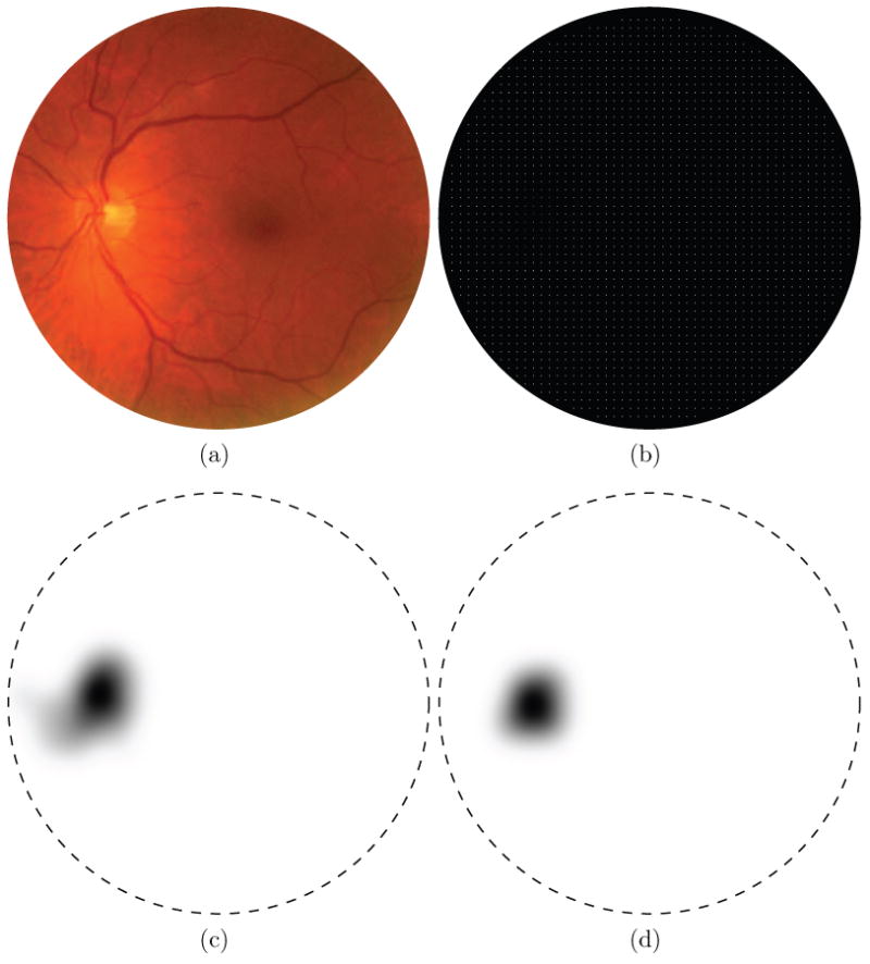
The optic disc detection step intermediate results. In the distance maps the border of the FOV is indicated by the dashed line. a) A color fundus photograph. b) The 10 × 10 optic disc search grid, sampling points are represented by the bright pixels c) Blurred distance map, result of rough grid search for the optic disc center (lower intensity equals lower distance). d) Blurred distance map of fine grid search for the optic disc center.

Based on the final optic disc location two foveal search areas are defined, one for the case the image is obtained from the left eye and one for the right eye case. In the left eye fundus image the fovea is located to the right of the optic disc and vice versa for the right eye fundus image. As it is unknown a priori whether the method is being applied to a left or a right eye, both search areas need to be processed. Parts of the search area outside the FOV are not processed to save time. The search area has been defined as follows, we determined the location of the fovea with respect to the optic disc in the 500 images in the training set. Based on this data we defined a rectangular search area that encompasses all fovea locations in the training set. We superimpose a 5 × 5 pixel grid over both search areas and determine dˆ for the fovea for each location on the grid (see Figure 6a). The remaining processing is the same as for the optic disc detection but without an additional refinement step and using r_Fovea instead of r_OD (see Figure 6b).

Fig. 6.

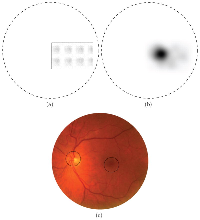
The fovea detection step intermediate results. In the distance maps the border of the FOV is indicated by the dashed line. a) The foveal search area (within the rectangle) based on the location of the optic disc, inside the search area each sampling position is indicated with a single dot. In this example the search area to the left of the optic disc lies outside the FOV and is therefore not processed or shown. b) After blurring, the pixel with the lowest value indicates the fovea location. c) The color fundus image from Figure 5a with the results superimposed. The circles are centered on the found locations.

4 Results

The method was applied to the pre-processed green plane image of all 600 test images. To determine our evaluation criteria we have looked at the criteria used in the literature. Counting optic disc detections inside the diameter of the optic disc as a true detection is an accepted evaluation method used by several of the references provided in the introduction (e.g. [9–11]). As far as the fovea is concerned, the border of the fovea region is not well defined and most of the work in the literature has also used the distance to the fovea center as an evaluation measure (e.g. [9–11]). For our application, diabetic retinopathy screening, knowing only the approximate centerpoint of both structures is adequate as we are not interested in the exact segmentation of the optic disc but simply want to mask it.

For each image we determined whether the optic disc location found by the algorithm was inside the border of the optic disc as indicated in the ground truth. For the fovea we determined if it was indicated within 40 pixels of the true location. The results of the experiments are given in Table 2. Several different splits of the data have been made. The “Set 1” section of the table shows the result of the system on all 500 regular screening images. In the “Set 2” row the results of the regular screening images in which the center of the fovea was inside the FOV are shown. In 51 optic disc centered screening images the fovea center was not within the field of view leaving 449 images in Set 2. The row marked “Set 3” contains the results on the 100 abnormal images, in all these images the fovea was within the field of view. A second observer also indicated the optic disc center and the fovea center in all test images. When the fovea center was outside the FOV the observer estimated its position. The results of this second observer are also included in Table 2. All positioning errors ε are given in pixels. To graphically show the results, a boxplot was produced for those cases where the positioning error was smaller than 50 pixels (see Figure 7). A comparison of the system performance with the second observer is also included.

Table 2.

The results of the proposed method measured against both the reference standard (i.e. the first observer) as well as against the second observer and the results of the second observer against the reference standard. All positioning errors ε are in pixels. From left to right the table shows the percentage of cases in which the structure was successfully located (accuracy), the mean positioning error, the median positioning error, the maximum positioning error, the minimum positioning error, the first quartile and the third quartile. Set 1 are the 500 regular screening images, Set 2 are the regular screening images in which the center of the fovea is inside the FOV and Set 3 are the images containing abnormalities.

Proposed Method vs. Reference Standard
Dataset	Accuracy	ε̄	ε̃	max(ε)	min(ε)	Q1	Q3
Set 1 optic disc	99.4%	8.4	7.2	150.0	1.0	4.2	10.3
Set 2 optic disc	99.4%	8.6	7.2	150.0	1.0	4.3	10.6
Set 3 optic disc	93.0%	20.5	9.9	250.5	1.0	5.8	15.1
Set 1 fovea	93.4%	28.9	6.4	514.5	0.0	3.6	10.7
Set 2 fovea	96.8%	16.1	6.0	514.5	0.0	3.6	9.2
Set 3 fovea	89.0%	25.4	7.3	479.6	0.0	4.5	14.6
Proposed Method vs. Second Observer
Dataset	Accuracy	ε̄	ε̃	max(ε)	min(ε)	Q1	Q3
Set 1 optic disc	99.6%	11.3	9.4	170.7	1.0	6.1	13.5
Set 2 optic disc	99.6%	11.4	9.4	170.7	1.0	6.1	13.5
Set 3 optic disc	93.0%	23.6	10.1	260.5	1.0	6.8	15.0
Set 1 fovea	93.2%	28.4	6.5	502.4	0.0	4.1	12.2
Set 2 fovea	94.8%	21.9	6.4	502.4	0.0	4.1	10.8
Set 3 fovea	87.0%	36.4	7.2	512.7	1.0	5.0	12.2
Second Observer vs. Reference Standard
Dataset	Accuracy	ε̄	ε̃	max(ε)	min(ε)	Q1	Q3
Set 1 optic disc	100.0%	8.3	7.3	43.5	0.5	4.5	10.8
Set 2 optic disc	100.0%	8.3	7.3	43.5	0.5	4.5	10.9
Set 3 optic disc	100.0%	4.8	4.1	16.6	1.0	2.2	6.1
Set 1 fovea	97.8%	7.5	4.3	82.5	0.2	2.7	7.6
Set 2 fovea	98.7%	6.9	4.1	82.5	0.2	2.4	6.9
Set 3 fovea	95.0%	9.6	5.4	67.7	0.0	3.2	10.3

Fig. 7.

A boxplot for both the proposed method (PM) and second observer (2O), of the cases in which ε was lower than 50 pixels. Indicated are the min, max, the median (white line), the mean (red diamond), the first and third quartile. To derive a meaningful boxplot from the data, outliers with a positioning error greater than 50 pixels were removed. From left to right 2, 2, 4, 0, 0, 0, 32, 15, 11, 7, 7 and 3 cases were removed.

5 Discussion and Conclusion

An automatic system for the detection of the location of the optic disc and the fovea has been presented. The system uses a kNN-regressor and a circular template to estimate the distance to a location in the image. It first finds the optic disc and then searches for the fovea based on the optic disc location. The performance of the system is good, in a heterogeneous set of regular screening images it successfully detected the location of the optic disc and the fovea in 99.4% and 93.4% of all 500 cases respectively. The set contained images from different cameras, with different resolutions and different degrees of coverage of the retina. After exclusion of those optic disc centered images in which the fovea itself is not visible, the detection performance for the fovea increases to 96.8%. For the set of pathological images the performance was lower but still good with a detection accuracy of 93.0% and 89.0% for the optic disc and fovea respectively. These performance numbers are comparable to the state of the art (see Section 1). Some representative results are shown in Figure 8a-f.

Fig. 8.

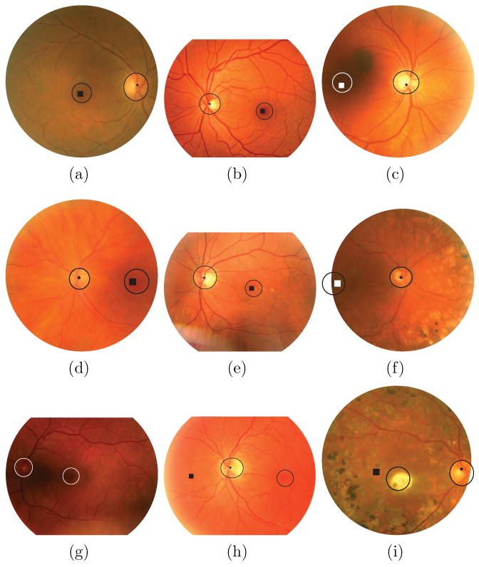
Example results, in each image the locations detected by the proposed method are shown by the dot (optic disc) and the square (fovea). The two circular objects in the image, one around the optic disc and one around the fovea, represent the areas of the image that are used for the detection accuracy determination. That is, whenever the algorithm detects the appropriate location anywhere within the indicated regions it is counted as a correct detection. The circles around the optic disc indicate the border of the optic disc while the fovea circles have a standard size (radius is 40 pixels). Differences in the apparent size of the fovea circles between images are due to scaling for display. a-d) Representative, correct results from Set 2. e-f) Representative, correct results from Set 3. g) No markers are shown due to complete failure of the method. h) The optic disc was detected successfully but the algorithm failed to identify the fovea position. i) Again the optic disc was found successfully but the fovea detection failed.

When comparing the results of the computer system with those of the second human observer on the ground truth, the most striking difference is in the positioning error of the fovea. This indicates that detection of the fovea position is a more difficult task and this is illustrated by the fact that the second human observer does not have a 100% detection performance in any of the sets of test images. Due to the way in which the system is designed, fovea detection failures tend to have large positioning errors. In all images two foveal search areas are defined, one to the left and one to the right of the optic disc. When the fovea is found in the wrong search area, the distance between the true fovea location and the found fovea location is large. Fovea detection failure is more likely to happen in optic disc centered images: of the 15 images in Set 2 in which fovea detection failed, 10 were optic disc centered images. This is likely due to the fact that the foveal search area is up to twice as large as in macula centered images (i.e. one search area to the left and one to the right of the optic disc) and the fovea can be located on either side of the optic disc. Optic disc localization failure also often leads to fovea localization failure: in Set 3 in all 7 cases where the optic disc was not successfully found, the fovea was not correctly localized as well. For the optic disc the localization error in general is low and comparable to that of the second human observer. In Set 1 and 2 the median localization error, the first quartile and the third quartile for detection of the optic disc of the second human observer and the algorithm are essentially the same. The mean is slightly higher for the algorithm due to the fact the few errors the algorithm makes tend to be large as illustrated by the maximum error of 150 pixels. The fact that the system obtains very similar results when compared with the second observer instead of with the ground truth is also an indication that, even though the system was trained with the ground truth, it is not overtrained on the observer who defined the ground truth in our experiment.

Since we have run the proposed algorithm on the same dataset as the system we previously described in [10] we can do a direct comparison. That system found the optic disc in 98.4% and the fovea in 94.4% in Set 1, 98.3% of the optic discs and 94.0% of the foveas in Set 2 and in Set 3 it found the optic disc in 94.0% and the fovea in 92% of all cases. For detection of the optic disc the proposed system has a better performance for Set 1 and 2 and performs slightly worse on Set 3 although the difference is just a single image. After analysis these differences proved not significant (where significant is defined as p <= 0.05). For the fovea in Set 1 the system from [10] performs better although the difference is not significant (p < 0.30), for Set 2 the proposed system is significantly (p < 0.01) better than the method from [10] and for the abnormal image data the system from [10] outperforms the proposed system but not significantly (p < 0.31). Thus, in images where the fovea is visible and that do not contain heavy pathology the proposed system is significantly better in detecting the fovea. This illustrates that fovea localization can benefit from using global image information such as the position of the vascular arch in cases where the fovea is completely obscured or is barely visible. The vascular arch can then be used to infer the approximate location of the fovea, something the proposed system does not do.

A large advantage of the proposed system is its speed. The proposed system demonstrates very similar or better performance and runs substantially faster than the one described in [10]. The average runtime on a single core of an Intel Core 2 Duo 2.83GHz is 7.6 seconds, the implementation was in C++. This average runtime includes pre-processing but does not include the time it takes to calculate the vessel segmentation. We expect to implement the proposed technique in an existing automatic screening system for diabetic retinopathy and a segmentation of the vasculature is given in this case as it is used for various purposes by the screening system [6]. If the vessel segmentation we used is included, it adds approximately 20 seconds to the total runtime. Even including the vessel segmentation time, the proposed method is faster than other methods reported in the literature (10 minutes for [10] and 2 minutes for [11], note that these algorithms were not run on the same hardware).

The feature selection procedure offers a view on which features are the most important for localizing the optic disc and the fovea. An interesting fact is that the selected features for both the optic disc and the fovea templates are almost completely symmetrical. For the optic disc the only non-symmetrical feature is the “number of vessels” feature which is selected in the neighboring quadrants I and IV. Otherwise the features are either selected for all quadrants or for opposing quadrants (i.e. the “Orientation of the vessel with maximum width”). For the fovea template all vessel features are only selected in opposing quadrants I and III. This makes intuitive sense because both left and right eyes are included in the training and testing sets. The fact no vessel features were selected for quadrants II and IV is somewhat surprising. Even though the fovea is in an area of the retina in which no visible vessels are present, to estimate the distance to the fovea at some location away (i.e. up to r_fovea pixels away) from its center the use of vessel features should be beneficial. Perhaps the use of relatively low resolution images (after pre-processing) as well as issues with the image quality (all images were acquired without mydriasis) were preventing successful extraction of the vessel features from the small vessels around the fovea. Nevertheless, the relatively low resolution does not seem to seriously affect the detection performance of the fovea detector in our test data.

We have carefully examined the cases in which the optic disc detector did not find the optic disc and the cases in which the fovea was not correctly localized but was visible in the image. The majority of failed detections are caused by poor contrast, poor quality vessel segmentation, imaging artifacts and the presence of pathology or a combination of these factors. When the contrast over the optic disc is low this not only affects the intensity features but also the vessel segmentation result. This combination of factors prevents the system from extracting good features for optic disc localization. In some cases the fovea detection fails when the fovea is just barely visible at the edge of the image or when there are artifacts/pathology covering the fovea (see Figure 8i). Figure 8g-i shows some examples of images on which the algorithm failed to find the correct location of the optic disc and/or the fovea. An example of low contrast over the optic disc causing complete failure of the method to find the optic disc and the fovea is shown in Figure 8g. Figure 8h shows an example of a flash artifact to the left of the optic disc, at the edge of the FOV (the bright band) causing an incorrect detection of the fovea. Because the flash artifact is bright it disturbs the intensity measurements in a large area to the left of the optic disc resulting in a large number of low distance estimates. The lowest predicted distance to the fovea was at the correct position but after the blurring step the lowest estimate was on the other side of the optic disc.

For our screening application, the main effect of a misdetected optic disc is that it will not be masked out correctly. This will in turn lead the abnormality detection algorithms to detect abnormalities on the optic disc location. This can cause an otherwise normal image to be flagged as “potentially abnormal” which in turn would lead to more work for the screening ophthalmologist who would have to look at the image. The result of a failed fovea detection is hard to predict. One of the main reasons to detect the fovea is that the location of a lesion with respect to the fovea plays a role in the determination of its severity. However, it is unlikely the automated screening will miss lesions based purely on their location with respect to the retina. The current performance of the optic disc and fovea detection system leads us to believe it is ready to be applied in our automated diabetic retinopathy screening system.

As we have used a heterogeneous set of images from different cameras and different coverage of the retina for training and testing the method has shown to be robust against different image types. Also, the method does not have any parameters that need tuning in case of application to other images. As long as the pre-processing step is done so that the FOV is resized to a standard size, the images are digital color fundus photographs and the coverage of the FOV is either 35 or 45 degrees, the system should not have to be retrained and the parameter settings as described in the paper can be applied.

To summarize, a robust, fast method to detect the position of the optic disc and the fovea in retinal images was presented. The method shows results comparable to state of the art methods, does not make strong assumptions about the location of both anatomical landmarks in the image and has an average runtime of around 20 seconds. This makes the system fit for employment in an automated screening system for diabetic retinopathy.

References

- 1.Niemeijer M, van Ginneken B, Russel S, Suttorp-Schulten M, Abràmoff MD. Automated detection and differentiation of drusen, exudates, and cotton-wool spots in digital color fundus photographs for diabetic retinopathy diagnosis. Investigative Ophthalmology & Visual Science. 2007;48:2260–2267. doi: 10.1167/iovs.06-0996. [DOI] [PMC free article] [PubMed] [Google Scholar]
- 2.Abràmoff MD, Alward WLM, Greenlee EC, Shuba L, Kim CY, Fingert JH, Kwon YH. Automated segmentation of the optic disc from stereo color photographs using physiologically plausible features. Invest Ophthalmol Vis Sci. 2007 Apr;48(no 4):1665–1673. doi: 10.1167/iovs.06-1081. [Online]. Available: http://dx.org/10.1167/iovs.06-1081. [DOI] [PMC free article] [PubMed]
- 3.Early Treatment Diabetic Retinopathy Study Research Group. Early Photocoagulation for Diabetic Retinopathy: ETDRS report 9. Ophthalmology. 1991;98:766–785. [PubMed] [Google Scholar]
- 4.Klonoff D, Schwartz D. An economic analysis of interventions for diabetes. Diabetes Care. 2000;23(no 3):390–404. doi: 10.2337/diacare.23.3.390. [DOI] [PubMed] [Google Scholar]
- 5.Abràmoff MD, Niemeijer M, Suttorp-Schulten MSA, Viergever MA, Russell SR, van Ginneken B. Evaluation of a system for automatic detection of diabetic retinopathy from color fundus photographs in a large population of patients with diabetes. Diabetes Care. 2008;31(no 2):193–198. doi: 10.2337/dc08-0952. [DOI] [PMC free article] [PubMed] [Google Scholar]
- 6.Niemeijer M, Abràmoff MD, van Ginneken B. Information fusion for diabetic retinopathy CAD in digital color fundus photographs. IEEE Transactions on Medical Imaging. 2009;28(no 5):775–785. doi: 10.1109/TMI.2008.2012029. [DOI] [PubMed] [Google Scholar]
- 7.Abdel-Razik Youssif AAH, Ghalwash AZ, Abdel-Rahman Ghoneim AAS. Optic disc detection from normalized digital fundus images by means of a vessels' direction matched filter. IEEE Transactions on Medical Imaging. 2008;27(no 1):11–18. doi: 10.1109/TMI.2007.900326. [DOI] [PubMed] [Google Scholar]
- 8.Foracchia M, Grisan E, Ruggeri A. Detection of optic disk in retinal images by means of a geometrical model of vessel structure. IEEE Transactions on Medical Imaging. 2004;23(no 10):1189–1195. doi: 10.1109/TMI.2004.829331. [DOI] [PubMed] [Google Scholar]
- 9.Tobin K, Chaum E, Govindasamy V, Karnowski T. Detection of anatomic structures in human retinal imagery. IEEE Transactions on Medical Imaging. 2007;26(no 12):1729–1739. doi: 10.1109/tmi.2007.902801. [DOI] [PubMed] [Google Scholar]
- 10.Niemeijer M, Abràmoff MD, van Ginneken B. Segmentation of the optic disc, macula and vascular arch in fundus photographs. IEEE Transactions on Medical Imaging. 2007;26:116–127. doi: 10.1109/TMI.2006.885336. [DOI] [PubMed] [Google Scholar]
- 11.Fleming AD, Goatman KA, Philip S, Olson JA, Sharp PF. Automatic detection of retinal anatomy to assist diabetic retinopathy screening. Phys Med Biol. 2007;52(no 2):331–345. doi: 10.1088/0031-9155/52/2/002. [Online]. Available: http://dx.org/10.1088/0031-9155/52/2/002. [DOI] [PubMed]
- 12.Sinthanayothin C, Boyce J, Cook H, Williamson T. Automated localisation of the optic disc, fovea, and retinal blood vessels from digital colour fundus images. British Journal of Ophthalmology. 1999;83:902–910. doi: 10.1136/bjo.83.8.902. [DOI] [PMC free article] [PubMed] [Google Scholar]
- 13.Li H, Chutatape O. Automated feature extraction in color retinal images by a model based approach. IEEE Transactions on Biomedical Engineering. 2004;51(no 2):246–254. doi: 10.1109/TBME.2003.820400. [DOI] [PubMed] [Google Scholar]
- 14.Cootes T, Taylor C, Cooper D, Graham J. Active shape models – their training and application. Computer Vision and Image Understanding. 1995;61(no 1):38–59. [Google Scholar]
- 15.Abràmoff MD, Suttorp-Schulten MSA. Web-based screening for diabetic retinopathy in a primary care population: the EyeCheck project. Telemed J E Health. 2005;11(no 6):668–674. doi: 10.1089/tmj.2005.11.668. [DOI] [PubMed] [Google Scholar]
- 16.Niemeijer M, Staal J, van Ginneken B, Loog M, Abràmoff MD. Comparative study of retinal vessel segmentation methods on a new publicly available database. Proceedings of SPIE: Medical Imaging. 2004;5370:648–656. [Google Scholar]
- 17.Staal J, Abràmoff MD, Niemeijer M, Viergever M, Van Ginneken B. Ridge based vessel segmentation in color image of the retina. IEEE Transactions on Medical Imaging. 2004;23(no 4):501–509. doi: 10.1109/TMI.2004.825627. [DOI] [PubMed] [Google Scholar]
- 18.Heijden Fvd, Duin RPW, Ridder Dd, Tax DMJ. Classification, Parameter Estimation and State Estimation: An Engineering Approach Using MATLAB. John Wiley and Sons; 2004. [Google Scholar]
- 19.van Ginneken B, Loog M. Pixel Position Regression - Application to medical image segmentation. In: Kittler J, Petrou M, Nixon M, editors. International Conference on Pattern Recognition; 2004. pp. 718–721. [Google Scholar]
- 20.Devroye L, Györfi L, Lugosi G. A Probabilistic Theory of Pattern Recognition. New York, USA: Springer-Verlag; 1996. [Google Scholar]
- 21.Duda RO, Hart PE, Stork DG. Pattern Classification. 2nd. New York: John Wiley and Sons; 2001. [Google Scholar]
- 22.Ahmed M, Ward R. A rotation invariant rule-based thinning algorithm for character recognition. IEEE Transactions on Pattern Analysis and Machine Intelligence. 2002;24(no 12):1672–1678. [Google Scholar]
- 23.Rockett P. An improved rotation-invariant thinning algorithm. IEEE Transactions on Pattern Analysis and Machine Intelligence. 2005;27(no 10):1671–1674. doi: 10.1109/TPAMI.2005.191. [DOI] [PubMed] [Google Scholar]
- 24.Pudil P, Novovicova J, Kittler J. Floating search methods in feature selection. Pattern Recognition Letters. 1994;15(no 11):1119–1125. [Google Scholar]
- 25.Perez-Rovira A, Trucco E. Robust optic disc location via combination of weak detectors. Proc 30th Annual International Conference of the IEEE Engineering in Medicine and Biology Society EMBS 2008; 20–25 Aug. 2008; pp. 3542–3545. [DOI] [PubMed] [Google Scholar]