Suite of finite element algorithms for accurate computation of soft tissue deformation for surgical simulation

Abstract

Real time computation of soft tissue deformation is important for the use of augmented reality devices and for providing haptic feedback during operation or surgeon training. This requires algorithms that are fast, accurate and can handle material nonlinearities and large deformations. A set of such algorithms is presented in this paper, starting with the finite element formulation and the integration scheme used and addressing common problems such as hourglass control and locking. The computation examples presented prove that by using these algorithms, real time computations become possible without sacrificing the accuracy of the results. For a brain model having more than 7000 degrees of freedom, we computed the reaction forces due to indentation with frequency of around 1000 Hz using a standard dual core PC. Similarly, we conducted simulation of brain shift using a model with more than 50 000 degrees of freedom in less than a minute. The speed benefits of our models results from combining the Total Lagrangian formulation with explicit time integration and low order finite elements.

1 Introduction

Systems using augmented reality for image guided surgery are important tools that can help surgeons improve the accuracy and limit the adverse effects of surgery. The existing imaging technology, such as MRI, provides good quality pre-operative images that can be used in such systems. These images can be analysed and registered on the real organs so that the surgeon can visualize the targeted area while the procedure is progressing.

Another area where fast computational algorithms are required is surgical simulation systems that provide visual and haptic feedback to the surgeon. Various haptic interfaces for medical simulation are especially useful for training surgeons for minimally invasive procedures (laparoscopy/interventional radiology) and remote surgery using tele-operators. These systems must compute the interaction force between the robotic tool and the tissue and provide it to the surgeon at frequencies of at least 500 Hz (DiMaio and Salcudean, 2005).

Biomechanical models are used for solving the haptic feedback problems, but many of these models are simplified in order to decrease the computational effort, e.g. they consider only infinitesimal deformations and/or linear material laws. These simplifications have a great influence on the accuracy of the obtained results in a finite element analysis, inducing significant errors (Carey, 1974; Martin and Carey, 1973; Oden and Carey, 1983). Biological tissues behaviour can be described in general using hyper-elastic or hyper-visco-elastic models (Fung, 1993). Therefore the solution method must be able to handle large deformations and nonlinear material models.

There are three ways the computation time can be reduced: by improving the algorithms, by using faster hardware or by using parallel computing. We will concentrate on the first method, as the use of faster hardware is limited by the existing technology and the use of parallel computing leads to more complex and more expensive hardware and software systems.

The paper is organized as follows: the proposed algorithms are presented in Section 2, computational examples that demonstrate the efficiency and accuracy of these algorithms are shown in Section 3 and the conclusions are presented in Section 4.

2 Finite element algorithms

When designing a finite element solution method there are many aspects that must be considered, such as the formulation used (Total or Updated Lagrangian), time integration scheme and the type of elements used for constructing the mesh. We will discuss these aspects in this section.

2.1 Integration of the equations of continuum mechanics

Various spatial discretization schemes are possible while using the finite element method (Belytschko, 1983). The algorithms implemented in the great majority of commercial finite element programs use the Updated Lagrangian formulation, where all variables are referred to the current (i.e. from the end of the previous time step) configuration of the system (Ansys (ANSYS), ABAQUS (ABAQUS, 1998), ADINA (ADINA R&D), LS-DYNA (Hallquist, 2005), etc.). The advantage of this approach is the simplicity of incremental strain description and low internal memory requirements. The disadvantage is that all derivatives with respect to spatial coordinates must be recomputed in each time step, because the reference configuration is changing. The reason for the popularity of Updated Lagrangian formulation seems to be historical – at the time of development of commercial finite elements solvers in the 1980s, computer memory was expensive. The internal memory cost is no longer a prohibitive factor so in developing our finite element algorithms we used the Total Lagrangian formulation, where all variables are referred to the original configuration of the system. We also use Second-Piola Kirchoff stress and Green. The decisive advantage of this formulation is that all derivatives with respect to spatial coordinates are calculated with respect to the original configuration and therefore can be pre-computed. The proposed stress and strain measures are appropriate for handling geometric nonlinearities (finite deformations).

The use of Total Lagrangian explicit integration for simulating physically realistic deformations was also proposed in (Zhuang and Canny, 1999). A method for decreasing the computation time when using non-linear elasticity was presented in (Picinbono et al., 2003), but it only works for tetrahedral meshes and special elastic material laws.

Because biological tissue behaviour can be described in general using hyper-elastic or hyper-visco-elastic models (Fung, 1993), the use of the Total Lagrangian formulation also leads to a simplification of material law implementation as these material models can be easily described using the deformation gradient. The stress is evaluated at each integration point based on the strains and any constitutive material model can be used, including time dependent material laws.

The integration of equilibrium equations in the time domain can be done using either implicit or explicit methods (Bathe, 1996; Belytschko, 1976; Crisfield, 1998). The most commonly used implicit integration methods, such as Newmark’s constant acceleration method, are unconditionally stable. This implies that their time step is limited only by the accuracy considerations. However, the implicit methods require solution of set of nonlinear algebraic equations at each time step. Furthermore, iterations need to be performed for each time step of implicit integration to control the error and prevent divergence. Therefore, the number of numerical operations per each time step can be three orders of magnitude larger than for explicit integration (Belytschko, 1976).

On the other hand, in explicit methods, such as the central difference method, treatment of nonlinearities is very straightforward and no iterations are required. By using a lumped (diagonal) mass matrix, the equations of motion can be decoupled and no system of equations must be solved. Computations are done at the element level eliminating the need for assembling the stiffness matrix of the entire model. Thus, computational cost of each time step and internal memory requirements are substantially smaller for explicit than for implicit integration. There is no need for iterations anywhere in the algorithm. These features make explicit integration suitable for real time applications.

However, the explicit methods are only conditionally stable. Normally a severe restriction on the time step size has to be included in order to receive satisfactory simulation results. Stiffness of soft tissue is very low (Miller, 2002; Miller and Chinzei, 1997, 2002; Miller et al., 2000): e.g. stiffness of brain is about eight orders of magnitude lower than that of common engineering materials such as steel. Since the maximum time step allowed for stability is (roughly speaking) inversely proportional to the square root of Young’s modulus divided by the mass density (Hallquist, 2005), it is possible to conduct simulations of brain deformation with much longer time steps than in typical dynamic simulations in engineering, which was confirmed in our previous simulation of brain shift using the commercial finite element solver LS-DYNA (Wittek et al., 2005; Wittek et al., 2007). Therefore, when developing the suite of finite element algorithms for computation of soft tissue deformation, we combined Total Lagrange formulation with explicit time integration.

A detailed description of the Total Lagrange Explicit Dynamics [TLED] algorithm is presented in (Miller et al., 2007). The main benefits of the TLED algorithm are:

• allows pre-computing of many variables involved (e.q. derivatives with respect to spatial coordinates, hourglass control parameters),

• no accumulation of errors – increase stability for quasistatic solutions,

• Second-Piola Kirchoff stress and Green strain are used – appropriate for handling geometric non-linearities,

• easy implementation of the material law for hyper-elastic materials using the deformation gradient,

• straightforward treatment of non-linearities,

• no iterations required for a time step,

• no system of equations need to be solved,

• low computational cost for each time step,

• low internal memory requirements.

2.2 Computation grid: elements used in the finite element mesh

Because of the computation time requirement, the mesh must be constructed using low order elements that are not computationally intensive, such as the linear tetrahedron or the linear under-integrated hexahedron. The standard formulation of the linear tetrahedral element exhibits artificial stiffening, referred to in the literature as volumetric locking (Bathe, 1996) when used for incompressible (or almost incompressible) continua such as brain and other soft tissues. To reduce locking special countermeasures must be employed and therefore hexahedral elements are preferred when modelling the behaviour of soft organs.

Many algorithms are now available for fast and accurate automatic mesh generation using tetrahedral elements, but not for automatic hexahedral mesh generation (Owen, 1998; Owen, 2001; Viceconti and Taddei, 2003). Some template based meshing algorithms can be used for meshing different organs using hexahedrons (Castellano-Smith et al., 2001; Couteau et al., 2000; Luboz et al., 2005), but these types of algorithms only work for healthy organs. In case of severe pathologies (such as a brain tumour), such algorithms can not be used, as the shape, size and position of the pathology is unpredictable. This is one reason why many authors proposed the use of tetrahedral meshes for their models (Clatz et al., 2003; Clatz et al., 2005; Ferrant et al., 2000; Ferrant et al., 2002; Warfield et al., 2002). In order to automate the simulation process, mixed meshes (having both hexahedral and tetrahedral elements) with predominantly hexahedral elements are the most convenient.

The under-integrated hexahedral elements require the use of an hourglass control algorithm in order to eliminate the instabilities, known as zero energy modes, which arise from the one-point integration (Flanagan and Belytschko, 1981). Special algorithms for handling hourglass control for the hexahedral elements must be implemented.

2.3 Hourglass control

The use of one point quadrature schemes for stress integration results in certain deformation modes remaining stressless. These modes are called kinematic, or zero energy, modes in the literature and hourglass modes for the hexahedron and quadrilateral in the finite element literature (Bathe, 1996) - because of the deformation patterns they produce in a mesh (Fig. 1.a).

Fig. 1.

Compression of a hexahedron meshed with under-integrated elements a) Without hourglass control b) With successful hourglass control

The hourglass modes can be controlled by calculating hourglass forces that oppose the hourglass deformation modes. One of the most popular and powerful hourglass control algorithms, that is currently available in many commercial software finite element packages, is the one proposed in (Flanagan and Belytschko, 1981). This method is applicable for hexahedral and quadrilateral elements with arbitrary geometry undergoing large deformations. The result of applying this hourglass control mechanism can be clearly seen in Fig. 1.b.

Starting from the algorithm proposed by Flanagan and Belytschko we proved that the Total Lagrangian formulation is also recommended from the point of view of efficient hourglass control implementation, as many quantities involved can be pre-computed. We have shown in (Joldes et al., 2007) that the hourglass control forces for each element can be computed (in matrix form) as:

$${}_0{}^t\mathbf{F}^{\mathit{Hg}}=k_0{\mathbf{Y}}_0{\mathbf{Y}}^T{}_0{}^t\mathbf{u}$$ (1)

where k is a constant that depends on the element geometry and material properties, Y is the matrix of hourglass shape vectors and u is the matrix of current displacements. The notation from (Bathe, 1996) is used, where the left superscript represents the current time and the left subscript represents the time of the reference configuration, which is 0 for Total Lagrangian. In Equation (1) all quantities except u are constant and can be pre-computed, making the hourglass control mechanism very efficient from the computational point of view.

The effectiveness of the hourglass control mechanism summarized in Eq. (1) can be clearly seen in Fig. 1.b.

In Table 1 we present the mean, standard deviation and maximum values of the error in nodal position computed using the two models (with and without hourglass control) when compared with a “gold standard” solution obtained using fully integrated elements in Abaqus. The introduction of hourglass control leads to a visible reduction of the error, with the maximum error reduced from 5.5% to 1.4% of the applied displacement.

Table 1.

Mean, standard deviation and maximum values of the error in nodal position (applied displacement was 1, initial hexahedron height was 3)

Model	Mean	Standard deviation	Maximum
Without hourglass control	0.028	0.015	0.055
With hourglass control	0.006	0.004	0.014

2.4 Non-locking tetrahedral elements

In modelling of incompressible continua, artificial stiffening (often referred to as volumetric locking) afflicts many standard elements including the linear tetrahedral element. This phenomenon occurs also for nearly incompressible materials and therefore introducing slight compressibility does not solve the problem

By examining the two-dimensional case from Fig. 2, adapted from (Hughes, 2000), we can see that the incompressibility constrain applied to elements 1 and 2 make the displacement of node a impossible (u_a = 0). An analysis of the rest of the mesh can be done to conclude that, regardless of the magnitude of the loading, every node in the mesh must have zero displacements in order to enforce the incompressibility constrains.

Fig. 2.

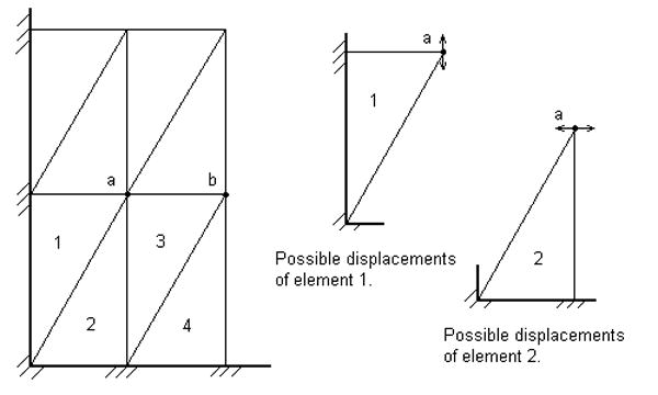
Mesh for which incompressibility dictates zero displacements. Adapted from (Hughes, 2000).

A number of improved linear tetrahedral elements with anti-locking features have been proposed by different authors (Bonet and Burton, 1998; Bonet et al., 2001; Dohrmann et al., 2000; Zienkiewicz et al., 1998). The average nodal pressure (ANP) tetrahedral element proposed in (Bonet and Burton, 1998) is computationally inexpensive and provides much better results for nearly incompressible materials compared to the standard tetrahedral element. Nevertheless, one shortcoming of the ANP element and its implementation in a finite element code is the handling of interfaces between different materials. We extended the formulation of the ANP element so that all elements in a mesh are treated in a similar way, requiring no special handling of the interface elements.

The ANP element defined in (Bonet, et al., 2001) is obtained by assuming that the volume ratio J remains constant over the volume attached to each node (instead of each element), therefore reducing the number of incompressibility constraints. The nodal volume ratio for a node a is defined in terms of current and initial nodal volumes as:

$$J_a=\frac{v_a}{V_a}$$ (2)

If only one material is considered, the average nodal pressure can be defined as:

$$p_a=\kappa (J_a-1)$$ (3)

The resulting element has the same deviatoric component of the strain energy as the standard tetrahedral element and a modified volumetric component. The modified volumetric component of the strain energy is computed in such a way that the element pressure for an element e is given as the average of the nodal pressures for the nodes belonging to that element:

$${\overline{p}}^{(e)}=\frac{1}{4}\sum _{a=1}^4{p}_a^{(e)}$$ (4)

In case of multiple material interfaces, the nodal pressure cannot be computed using (3), as it is not clear what bulk modulus κ should be used. For each material type i converging at node a, a different nodal volume is defined as:

$$v_a^{(i)}=\sum _{e=1}^{m_a^{(i)}}\frac{1}{4}{v}^{(e)}$$ (5)

where m_a⁽ⁱ⁾ represents the number of elements of material type i sharing node a. A different nodal pressure is then evaluated for each material as:

$$p_a^{(i)}={\kappa }^{(i)}(J_a^{(i)}-1)$$ (6)

When the pressures are averaged over an element, only those corresponding to the same element material are used.

The different treatment of elements having different material types at the interface nodes leads to:

• implementation problems, as not all elements in the mesh are treated in the same manner,

• a weaker enforcement of the incompressibility constraints for the nodes belonging to material interfaces (the elements of different material type are treated separately).

Instead of considering different nodal pressure for different material types (as given by (6)) we make the assumption that the nodal pressure is constant over the nodal volume. This assumption derives from the relation that exists between pressure and stress (p =-σ_ii/3) (Hughes, 2000) and from the fact that at the interface between two different materials the stress in the materials should be the same. Starting from this assumption, we demonstrated in (Joldes et al., 2008a) that the nodal pressure should be computed as:

$$p_a=\frac{\sum _{e=1}^{m_a}{p}^{(e)}{V}^{(e)}}{\sum _{e=1}^{m_a}{V}^{(e)}}$$ (7)

where m_a is the number of elements surrounding node a. The element pressure is computed afterwards in the same manner as for the standard ANP element, using (4).

In case of a node surrounded by elements made of the same material, the nodal pressure given by (7) reduces to (3). Therefore, the standard ANP element and the improved ANP element proposed by us behave differently only for elements situated at an interface between different materials.

Regarding the implementation, the ANP element only modifies the deviatoric component of the strain energy of the standard tetrahedral element, which in turn depends only on the volumetric part of the deformation gradient. Therefore we can obtain the desired behaviour of the ANP element by modifying the volumetric part of the deformation gradient of the standard tetrahedral element (the element Jacobian).

We compute the element Jacobian, required so that the element pressure (as given by 4) for the ANP element is obtained, using the following formula:

$${\overline{J}}^{(e)}=\frac{{\overline{p}}^{(e)}}{\kappa }+1$$ (8)

Because the element Jacobian is equal to the determinant of the element deformation gradient, we define a modified deformation gradient that has the same isochoric part as the normal deformation gradient, but the volumetric part is modified so that its determinant (and therefore the volumetric deformation) is equal to the required element Jacobian:

$${\overline{\mathbf{X}}}^{(e)}={\left({\overline{\mathit{J}}}^{(e)}\right)}^{1/3}{\left({\mathit{J}}^{(e)}\right)}^{-1/3}\mathbf{X},{\mathit{J}}^{(e)}=\det (\mathbf{X})$$ (9)

The computation of the nodal forces (or stiffness matrix) can now be done in the usual manner, but using the modified deformation gradient instead of the normal deformation gradient for defining the strains. This way any existing material law implementation can be used.

2.5 Modelling of interactions between different organs: contact algorithm

Many simulations require the treatment of interactions between different parts of the model. In order to handle the brain-skull interaction we developed a very efficient algorithm that treats this interaction as a finite sliding, frictionless contact between a deformable object (the brain) and a rigid surface (the skull). The contact type was chosen based on the anatomical properties of the brain-skull interface. The brain is surrounded by cerebrospinal-fluid (CSF) inside the skull and we considered that a complete CSF drainage takes place after craniotomy, allowing the brain to enter into contact and easily slide along the skull (Hu et al., 2007; Skrinjar et al., 2002).

Unlike contacts in commercial finite element solvers (e.g. Abaqus, LS-DYNA), our contact algorithm has no configuration parameters (as it only imposes kinematic restrictions on the movement of the brain surface nodes) and is very fast, with the speed almost independent of the mesh density for the skull surface.

The main parts of the contact algorithm are: detection of nodes on the brain surface (also called the slave surface) which have penetrated the skull surface (master surface) and the displacement of each slave node that has penetrated the master surface to the closest point on the master surface.

The surfaces of the anatomical structures of segmented brain images are typically discretised using triangles; therefore we consider the skull surface as a triangular mesh. We will call each triangle surface a “face”, the vertices - “nodes” and the triangle sides - “edges”.

We base our penetration detection algorithm on the closest master node (nearest neighbour) approach (Hallquist, 2005). The basic algorithm is as follows:

• - For each slave node P:

  • Find the closest master node C (global search)

  • Check the faces and edges surrounding C for penetration (local search)

To improve the computation speed, following (Hallquist, 2005), we implemented the global search phase using bucket sort. A good description of this searching algorithm is given in (Sauve and Morandin, 2004). In our implementation the size of the buckets used for the global search is different in the three directions, being given in each direction by half of the maximum size of the projections of all master edges on that direction. This ensures that the number of nodes in each bucket is minimal while there are no buckets for which a closest node cannot be found.

The next step (local search) aims at finding for each slave node P the closest node R (on the master surface) on the faces or edges surrounding node C. Once the closest point on the master surface is identified, the penetration is detected by checking the sign of the scalar product RP·n, with n the inside normal to the master surface in R. For an edge or a node the normal is defined as the sum of the normal vectors of adjacent faces.

In most of the cases, the basic tests presented above are sufficient for identifying the closest point on the master surface. Nevertheless, there are also special cases that must be considered, when the closest point on the master surface is not on the faces and edges adjacent to C. In commercial software this problem is solved by searching for the closest face or edge on the master surface instead of searching for the closest master node (Hallquist, 2005). This search is time consuming even if bucket sort is used. Therefore our proposal for handling these special cases is to make an analysis of the master surface and identify for each node C all the faces and edges that can be penetrated by a slave node P in the case C is the closest master node to P. This analysis is done based on geometrical considerations and is not detailed in this paper. A detailed description of this analysis is presented in (Joldes et al., 2008b). The identified faces and edges are kept in a list for each master node C and are checked in addition to the faces and edges that contain C when the local search is performed. Because the master surface is rigid this analysis can be done pre-operatively, greatly reducing the contact computation time during the intra-operative simulation.

3 Validation of the developed algorithms

The accuracy and reliability of the new algorithms is best assessed against existing, verified numerical procedures implemented in commercial finite element packages. Validation by modelling of an actual surgery may be compromised by many unknowns (e.g. patient-specific geometry, boundary conditions and material properties) involved in such a simulation. Therefore, we applied our algorithms in two simulations, a brain indentation and a brain shift, and compared the results with those obtained using the commercial solvers Abaqus and LS-DYNA.

The main focus of the brain indentation simulation was to verify the developed algorithms in terms of their accuracy in predicting reaction forces. The mesh we used had 2 428 nodes and 2 059 elements (2 023 under-integrated hexahedron and 36 improved tetrahedral elements in the indentation area - see Fig. 3). The results obtained using our algorithms were compared with those obtained using the commercial software package Abaqus. We selected the Abaqus package as it is regarded as one of the most accurate and reliable packages for predicting stresses in nonlinear continua.

Fig. 3.

Simulation of brain indentation – the mixed mesh is deformed by displacing 4 nodes. The colour code represents the differences in nodal displacements compared to the Abaqus simulation. Dimensions are in mm.

The indentation was simulated by displacing 4 nodes in the direction normal to the brain surface by 20 mm using a smooth loading curve. An almost incompressible nonlinear neo-Hookean material was used for the brain tissue (mass density of 1 000 kg/m³, Young’s modulus in un-deformed state equal to 3 000 Pa and Poisson’s ratio 0.49) and a compressible neo-Hookean material for the ventricle (mass density of 1 000 kg/m³, Young’s modulus in un-deformed state equal to 100 Pa and Poisson’s ratio 0.1). The same constraints as in (Wittek et al., 2004) were used and brain symmetry was assumed.

In Abaqus we used fully integrated mixed formulation elements for the mesh, which are the “gold standard” elements in case of almost incompressible materials simulations (ABAQUS, 1998). We used the implicit solver with the default configuration.

Computations were performed on a standard 3 GHz Intel® Core™ Duo CPU system using Windows XP operating system. The simulation consisted of 2 000 time steps and took less than 2s using our TLED method, giving a force feedback frequency of about 1 000 Hz. The Abaqus implicit simulation performed 100 time steps in about 3 minutes. There is very good agreement between the results obtained using our software and the results from the Abaqus simulation, in cases of both displacements and reaction forces (Fig. 4) – the displaced profiles almost overlap and the maximum relative error in reaction forces is 2.5%. The difference in nodal displacements between the two simulations (in mm) has a mean value of 0.02, a standard deviation of 0.03 and a maximum value of 0.92. The distribution of this difference on the brain surface is presented in Figure 3, where one can notice that the maximum error is obtained close to the area where the deformation is applied (being the result of high element distortion).

Fig. 4.

Computed displacements (a) and reaction forces (b) using Abaqus implicit solver and our algorithms

In another experiment we performed the registration of a patient specific brain shift. LS-DYNA simulations for this case have been done previously and the results were found to agree well with the MRI derived deformations (Wittek et al., 2008). The mesh was obtained from a pre-operative MRI and was deformed by applying displacements recovered in the area of the craniotomy from the intra-operative MRI image. The LS-DYNA simulation was altered by eliminating the self contact on the brain surface (between cerebellum and cerebrum), as this contact is not handled by our algorithm, but the changes to the model had little effect on the simulation results as the cerebellum is only loosely coupled to the rest of the brain through the brain stem. We performed the same simulations using our contact algorithm and TLED with mass proportional damping added in order to obtain the steady state solution. The difference in the nodal displacement field has a mean value of 0.4 mm, a standard deviation of 0.2 mm and a maximum value of 1.2 mm (including the nodes on the cerebellum) (Fig. 5).

Fig. 5.

Brain shift simulation – difference between the TLED and LS-DYNA results. The transparent mesh represents the master contact surface. The colour code represents the dif-ferences in nodal displacements between the two simulations. All dimensions are in mm.

The results presented in Table 2 show the very good agreement between the centre of gravity displacements obtained using LS-DYNA and our algorithms (maximum 0.5 mm difference). The computed deformations are also very close to the ones extracted from the intra-operative MRI considering that the accuracy of determining the MRI based deformations is limited by the voxel size in the MRI images used (in this case 0.85mm × 0.85mm × 2.5 mm).

Table 2.

Observed and computed centres of gravity displacements for ventricles and tumour [mm]

Model	Ventricles			Tumour
	ΔX	ΔY	ΔZ	ΔX	ΔY	ΔZ
Intra-operative MRI	3.4	0.2	1.7	5.5	-0.2	1.7
LS-DYNA	2.7	-0.2	2.3	5.6	-0.7	2.5
TLED	3.2	-0.3	2.2	5.7	-0.8	2.5

In Fig. 6 the results of the two simulations are compared with the intra-operative MRI for three transverse sections through the brain. We notice the good agreement between the simulation results in these cross sections. The differences between the computed and MRI derived intra-operative cross sections are also very small, but these differences are influenced by other errors (e.g. segmentation differences between pre- and intra-operative MRI images).

Fig. 6.

Brain shift simulation – comparison between the simulation results and the intra-operative MRI. The cutting sections are perpendicular to the superiorly pointing axis, with 0 on the brain’s most superior vertex, at distances of a) -45.5mm b) -50.5 mm and c) -55.5 mm. Grid lines are 5 mm apart.

The used mesh had 16 710 nodes and 15 050 elements. The computation time for 1000 time steps was about 12 s and less than 3 000 time steps were needed to reach the steady state solution. Therefore we need less than one minute for a complete brain shift simulation. For the same number of time steps, our simulation is at least 2 times faster than the LS-DYNA simulation.

For a master surface consisting of 1 993 nodes and 3 960 triangular faces and a slave surface having 1 749 nodes, the computation time dedicated to the contact handling for 1 000 time steps is about 3.2 s. If we refine the master surface and increase the number of triangles 4 times (to 15 840), the computation time for 1 000 time steps increases to 3.8 s. Therefore, the contacts computation time is almost independent of the number of triangles on the master surface.

4 Conclusions

In this paper we presented a suite of finite element algorithms that can be used for accurate and fast computation of soft tissue deformation for surgical simulation. The basic concept behind these algorithms is the use of the Total Lagrangian formulation for solving finite element problems. The presented algorithms cover issues related to time integration, hourglassing, volumetric locking and contacts. We use fully nonlinear formulation, accounting for large deformations, rigid body motions and material nonlinearities.

Explicit time integration is the preferred method for performing real time simulations. The treatment of nonlinearities is straightforward, without the need for any iterations. Even if the method is only conditionally stable, the material properties of biological soft tissues make possible the use of much larger time steps compared with other engineering applications. Nevertheless, in the case of very large deformations or high deformation speeds, some elements can become highly distorted, leading to a reduction of the critical time step. In such a case, monitoring of the critical time step is required and the simulation time step must be automatically adjusted (if a time accurate solution is needed) or the mass of the distorted elements can be scaled (if only the steady state solution is sought). On a dual core PC this can be done in a separate thread leading to only a slight increase in the computation time.

A very efficient hourglass control implementation is proposed for the under-integrated hexahedral element. Having only one integration point, this element is very inexpensive from the computational point of view, being a perfect candidate for real time surgical simulations. The possibility to use this type of element and the improved tetrahedral element in mix meshes is a step towards complete automated patient specific surgical simulation.

An improved version of the average nodal pressure tetrahedral element was developed. This improved formulation handles all the elements of the mesh in the same manner (including elements at an interface between materials) and therefore the use of different materials and the implementation in an existing finite element code can be made without difficulties.

We developed a very simple and efficient contact algorithm that can be used for simulating the brain-skull interaction. Because the skull is modelled as a rigid surface, it can be analyzed pre-operatively and many quantities needed for handling the contact can be pre-computed. No parameters are needed for defining the contact (contact thickness, stiffness, etc.) as it only imposes kinematic restrictions on the movement of the brain nodes. Such contact algorithm is needed for intra-operative brain shift simulations when only limited information about the brain surface deformation can be obtained from the craniotomy area.

The simulation examples confirm the speed and accuracy of the presented algorithms. We could compute reaction forces at frequencies of 1 000 Hz for a mesh having more than 2 000 hexahedral elements and perform a full brain shift simulation in less than a minute for a model having more than 50 000 degrees of freedom on a simple PC workstation. The accuracy of our results was demonstrated by comparing them with the results of similar simulations done using much more complex elements and contact algorithms in the commercial finite element software Abaqus and LS-DYNA. Good agreement (differences in displacement of an order of 0.2 mm) with the commercial finite element software results was obtained.

References

- 1.ABAQUS. ABAQUS Theory Manual, Version 5.8. Hibbitt: Karlsson & Sorensen, Inc.; 1998. [Google Scholar]
- 2.ADINA R&D, ADINA home page - www.adina.com.
- 3.ANSYS, ANSYS home page - www.ansys.com.
- 4.Bathe K-J. Finite Element Procedures. Prentice-Hall; New Jersey: 1996. [Google Scholar]
- 5.Belytschko T. A survey of numerical methods and computer programs for dynamic structural analysis. Nuclear Engineering and Design. 1976;37:23–34. [Google Scholar]
- 6.Belytschko T. An Overview of Semidiscretization and Time Integration Procedures. Computational Methods for Transient Analysis North-Holland, Amsterdam. 1983:1–66. [Google Scholar]
- 7.Bonet J, Burton AJ. A simple averaged nodal pressure tetrahedral element for incompressible and nearly incompressible dynamic explicit applications. Communications in Numerical Methods in Engineering. 1998;14:437–449. [Google Scholar]
- 8.Bonet J, Marriott H, Hassan O. An averaged nodal deformation gradient linear tetrahedral element for large strain explicit dynamic applications. Communications in Numerical Methods in Engineering. 2001;17:551–561. [Google Scholar]
- 9.Carey GF. A Unified Approach to Three Finite Element Theories for Geometric Nonlinearity. Journal of Computer Methods in Applied Mechanics and Engineering. 1974;4(1):69–79. [Google Scholar]
- 10.Castellano-Smith AD, Hartkens T, Schnabel J, Hose DR, Liu H, Hall WA, Truwit CL, Hawkens DJ, Hill DLG. Constructing patient specific models for correcting intraoperative brain deformation. 4th International Conference on Medical Image Computing and Computer Assisted Intervention MICCAI; 2001; Utrecht, The Netherlands. [Google Scholar]
- 11.Clatz O, Delingette H, Bardinet E, Dormont D, Ayache N. Patient Specific Biomechanical Model of the Brain: Application to Parkinson’s disease procedure. In: Ayache N, Delingette H, editors. International Symposium on Surgery Simulation and Soft Tissue Modeling (IS4TM’03) Juan-les-Pins, France: Springer-Verlag; 2003. [Google Scholar]
- 12.Clatz O, Sermesant M, Bondiau P-Y, Delingette H, Warfield SK, Malandain G, Ayache N. Realistic Simulation of the 3D Growth of Brain Tumors in MR Images Coupling Diffusion with Biomechanical Deformation. IEEE Trans Med Imaging. 2005;24(10):1334–1346. doi: 10.1109/TMI.2005.857217. [DOI] [PMC free article] [PubMed] [Google Scholar]
- 13.Couteau B, Payan Y, Lavallée S. The Mesh-Matching Algorithm: An Automatic 3D Mesh Generator fo Finite Element Structures. J Biomech. 2000;33:1005–1009. doi: 10.1016/s0021-9290(00)00055-5. [DOI] [PubMed] [Google Scholar]
- 14.Crisfield MA. Non-linear Finite Element Analysis of Solids and Structures. John Wiley & Sons; Chichester: 1998. Non-linear dynamics; pp. 447–489. [Google Scholar]
- 15.DiMaio SP, Salcudean SE. Interactive Simulation of Needle Insertion Models. IEEE Trans on Biomedical Engineering. 2005;52(7) doi: 10.1109/TBME.2005.847548. [DOI] [PubMed] [Google Scholar]
- 16.Dohrmann CR, Heinstein MW, Jung J, Key SW, Witkowski WR. Node-based uniform strain elements for three-node triangular and four-node tetrahedral meshes. International Journal for Numerical Methods in Engineering. 2000;47:1549–1568. [Google Scholar]
- 17.Ferrant M, Macq B, Nabavi A, Warfield SK. Deformable Modeling for Characterizing Biomedical Shape Changes. In: Borgefors ING, Sanniti di Baja G, editors. Discrete Geometry for Computer Imagery; 9th International Conference; 2000; Uppsala, Sweden, Springer-Verlag GmbH. [Google Scholar]
- 18.Ferrant M, Nabavi A, Macq B, Black PM, Jolesz FA, Kikinis R, Warfield SK. Serial registration of intraoperative MR images of the brain. Med Image Anal. 2002;6(4):337–359. doi: 10.1016/s1361-8415(02)00060-9. [DOI] [PubMed] [Google Scholar]
- 19.Flanagan DP, Belytschko T. A uniform strain hexahedron and quadrilateral with orthogonal hourglass control. International Journal for Numerical Methods in Engineering. 1981;17:679–706. [Google Scholar]
- 20.Fung YC. Biomechanics. Mechanical Properties of Living Tissues. Second. Springer-Verlag; New York: 1993. [Google Scholar]
- 21.Hallquist JO. LS-DYNA Theory Manual. Vol. 94551. Livermore Software Technology Corporation; Livermore, California: 2005. [Google Scholar]
- 22.Hu J, Jin X, Lee JB, Zhang L, Chaudhary V, Guthikonda M, Yang KH, King AI. Intraoperative brain shift prediction using a 3D inhomogeneous patient-specific finite element model. J Neurosurg. 2007;106:164–169. doi: 10.3171/jns.2007.106.1.164. [DOI] [PubMed] [Google Scholar]
- 23.Hughes TJR. The Finite Element Method: Linear Static and Dynamic Finite Element Analysis. Dover Publications; Mineola: 2000. [Google Scholar]
- 24.Joldes GR, Wittek A, Miller K. An Efficient Hourglass Control Implementation for the Uniform Strain Hexahedron Using the Total Lagrangian Formulation. Communications in Numerical Methods in Engineering. 2007 doi: 10.1002/cnm.1034. [DOI] [Google Scholar]
- 25.Joldes GR, Wittek A, Miller K. Non-locking Tetrahedral Finite Element for Surgical Simulation. Communications in Numerical Methods in Engineering. 2008a doi: 10.1002/cnm.1185. [DOI] [PMC free article] [PubMed] [Google Scholar]
- 26.Joldes GR, Wittek A, Miller K, Morriss L. Realistic And Efficient Brain-Skull Interaction Model For Brain Shift Computation. In: Miller K, Nielsen PMF, editors. Computational Biomechanics for Medicine III Workshop, MICCAI; 2008b; New-York. [Google Scholar]
- 27.Luboz V, Chabanas M, Swider P, Payan Y. Orbital and Maxillofacial Computer Aided Surgery: Patient-Specific Finite Element Models To Predict Surgical Outcomes. Comput Methods Biomech Biomed Engin. 2005;8(4):259–265. doi: 10.1080/10255840500289921. [DOI] [PubMed] [Google Scholar]
- 28.Martin HC, Carey GF. Introduction to Finite Element Analysis: Theory and Application. McGraw-Hill Book Co.; New York: 1973. [Google Scholar]
- 29.Miller K. Biomechanics of Brain for Computer Integrated Surgery. Publishing House of Warsaw University of Technology; Warsaw: 2002. [Google Scholar]
- 30.Miller K, Chinzei K. Constitutive modelling of brain tissue; Experiment and Theory. J Biomech. 1997;30(1112):1115–1121. doi: 10.1016/s0021-9290(97)00092-4. [DOI] [PubMed] [Google Scholar]
- 31.Miller K, Chinzei K. Mechanical properties of brain tissue in tension. J Biomech. 2002;35:483–490. doi: 10.1016/s0021-9290(01)00234-2. [DOI] [PubMed] [Google Scholar]
- 32.Miller K, Chinzei K, Orssengo G, Bednarz P. Mechanical properties of brain tissue in-vivo: experiment and computer simulation. J Biomech. 2000;33:1369–1376. doi: 10.1016/s0021-9290(00)00120-2. [DOI] [PubMed] [Google Scholar]
- 33.Miller K, Joldes GR, Lance D, Wittek A. Total Lagrangian Explicit Dynamics Finite Element Algorithm for Computing Soft Tissue Deformation. Communications in Numerical Methods in Engineering. 2007;23:121–134. [Google Scholar]
- 34.Oden JT, Carey GF. Finite Elements: Special Problems in Solid Mechanics. Prentice-Hall; 1983. [Google Scholar]
- 35.Owen SJ. A Survey of Unstructured Mesh Generation Technology. In: Lab SN, editor. 7th International Meshing Roundtable; 1998; Dearborn, Michigan, USA. [Google Scholar]
- 36.Owen SJ. Hex-dominant mesh generation using 3D constrained triangulation. Computer-Aided Design. 2001;33:211–220. [Google Scholar]
- 37.Picinbonos G, Delingette H, Ayache N. Non-linear anisotropic elasticity for real-time surgery simulation. Graphical Models. 2003;65:305–321. [Google Scholar]
- 38.Sauve RG, Morandin GD. Simulation of contact in finite deformation problems –algorithm and modelling issues. International Journal of Mechanics and Materials in Design. 2004;1:287–316. [Google Scholar]
- 39.Skrinjar O, Nabavi A, Duncan J. Model-driven brain shift compensation. Med Image Anal. 2002;6:361–373. doi: 10.1016/s1361-8415(02)00062-2. [DOI] [PubMed] [Google Scholar]
- 40.Viceconti M, Taddei F. Automatic generation of finite element meshes from computed tomography data. Crit Rev Biomed Eng. 2003;31(1):27–72. doi: 10.1615/critrevbiomedeng.v31.i12.20. [DOI] [PubMed] [Google Scholar]
- 41.Warfield SK, Talos F, Tei A, Bharatha A, Nabavi A, Ferrant M, Black PM, Jolesz FA, Kikinis R. Real-time registration of volumetric brain MRI by biomechanical simulation of deformation during image guided surgery. Computing and Visualization in Science. 2002;5:3–11. [Google Scholar]
- 42.Wittek A, Hawkins T, Miller K. On the unimportance of constitutive models in computing brain deformation for image-guided surgery. Biomech Model Mechanobiol. 2008 doi: 10.1007/s10237-10008-10118-10231. [DOI] [PMC free article] [PubMed] [Google Scholar]
- 43.Wittek A, Kikinis R, Warfield SK, Miller K. Brain shift computation using a fully nonlinear biomechanical model. 8th International Conference on Medical Image Computing and Computer Assisted Surgery MICCAI 2005; 2005; Palm Springs, California, USA. [DOI] [PubMed] [Google Scholar]
- 44.Wittek A, Miller K, Kikinis R, Warfield SK. Patient-Specific Model of Brain Deformation: Application to Medical Image Registration. J Biomech. 2007;40:919–929. doi: 10.1016/j.jbiomech.2006.02.021. [DOI] [PubMed] [Google Scholar]
- 45.Wittek A, Miller K, Laporte J, Kikinis R, Warfield SK. Computing reaction forces on surgical tools for robotic neurosurgery and surgical simulation. Australasian Conference on Robotics and Automation ACRA; 2004; Canberra, Australia. [Google Scholar]
- 46.Zhuang Y, Canny J. Real-time Simulation of Physically Realistic Global Deformation. IEEE Vis’99; 1999; San Francisco, California. [Google Scholar]
- 47.Zienkiewicz OC, Rojek J, Taylor RL, Pastor M. Triangles and Tetrahedra in Explicit Dynamic Codes for Solids. International Journal for Numerical Methods in Engineering. 1998;43:565–583. [Google Scholar]