Optimal Investment in HIV Prevention Programs: More Is Not Always Better

Abstract

This paper develops a mathematical/economic framework to address the following question: Given a particular population, a specific HIV prevention program, and a fixed amount of funds that could be invested in the program, how much money should be invested? We consider the impact of investment in a prevention program on the HIV sufficient contact rate (defined via production functions that describe the change in the sufficient contact rate as a function of expenditure on a prevention program), and the impact of changes in the sufficient contact rate on the spread of HIV (via an epidemic model). In general, the cost per HIV infection averted is not constant as the level of investment changes, so the fact that some investment in a program is cost effective does not mean that more investment in the program is cost effective. Our framework provides a formal means for determining how the cost per infection averted changes with the level of expenditure. We can use this information as follows: When the program has decreasing marginal cost per infection averted (which occurs, for example, with a growing epidemic and a prevention program with increasing returns to scale), it is optimal either to spend nothing on the program or to spend the entire budget. When the program has increasing marginal cost per infection averted (which occurs, for example, with a shrinking epidemic and a prevention program with decreasing returns to scale), it may be optimal to spend some but not all of the budget. The amount that should be spent depends on both the rate of disease spread and the production function for the prevention program. We illustrate our ideas with two examples: that of a needle exchange program, and that of a methadone maintenance program.

1. Introduction

In 2007, an estimated 2.5 million new cases of human immunodeficiency virus (HIV) occurred worldwide, bringing the total number of people living with HIV/AIDS to 33 million [1]. However, funds for HIV prevention fall far short of the estimated need [2], so it is crucial to make the best use of available prevention funds.

A key question faced by decision makers is how much to spend on any given HIV prevention program. In general, the relationship between expenditure on a prevention program and HIV infections averted is not linear: preventing one infection may in the long run prevent many other infections. Moreover, each incremental dollar spent on prevention may not generate the same incremental reduction in HIV transmission risk. At low levels of expenditure, increased investment in a prevention program may generate increasingly greater reductions in transmission risk until an effective program level has been reached (for example, a counseling session that is long enough to be effective). At a high enough level of expenditure, increased investment may yield diminishing levels of incremental risk reduction (for example, if the program has already reached those individuals who are the most willing to change their behavior).

Due to these complexities, and to lack of sufficient knowledge about the effectiveness of prevention programs and the behavioral and other factors driving the HIV epidemic in any given region, decision makers often make the simplifying assumption (either explicitly or implicitly) that the benefits of prevention programs grow linearly with funds invested [3, 4]. For a single prevention program, the assumption of linearity leads naturally to the following rule of thumb: if it is worth investing in the prevention program, it is worth investing the maximum amount possible. However, more investment may not always be better. A prevention program that is cost effective at low levels of expenditure can become less so with additional expenditure if the additional expenditure does not cause a proportional increase in benefit. Conversely, a prevention program that does not appear to be cost effective at a low level of expenditure might be cost effective at a higher level of expenditure.

To make an informed decision about how much money to invest in a particular HIV prevention program, decision makers need to know how many infections are likely to be prevented for each level of expenditure. Cost-effectiveness analyses (and cost-benefit and cost-utility analyses) often evaluate specific HIV prevention programs retrospectively, considering a single level of program expenditure [5-9]. The results of such analyses cannot easily be scaled to different levels of expenditure because it is not known how much additional benefit would be gained (or lost) through additional (or less) expenditure.

Some analyses have evaluated the incremental cost effectiveness of different components of HIV prevention programs (e.g., a safer-sex lecture only vs. a safer-sex lecture coupled with skills training [10]; bottle feeding vs. bottle feeding and antiretroviral treatment at birth or Caesarian delivery [11, 12]). However, such analyses do not determine how the results would change for different levels of expenditure on each component. Kaplan [13] explored optimal funding questions for needle exchange programs, but under the limiting assumptions of a short time horizon with constant HIV prevalence and decreasing marginal numbers of injection drug users reached as a function of total expenditure. Other authors have applied optimization techniques to explore the optimal allocation of prevention funds across multiple populations and programs [14-21], but the results of such analyses do not provide insight into the optimal level of expenditure on a single prevention program.

This paper develops a mathematical/economic framework to address the following question: Given a particular population, a specific HIV prevention program, and a fixed amount of funds that could be invested in the program, how much money should be invested? We consider the impact of investment in a prevention program on the HIV sufficient contact rate (defined via production functions that describe the change in the sufficient contact rate as a function of expenditure on a prevention program), and the impact of changes in the sufficient contact rate on the spread of HIV (via an epidemic model). For any level of expenditure, we measure the number of cases of HIV averted over a fixed time horizon. A previous study [22] showed how simulation can be used to evaluate different levels of investment in an HIV prevention program, with the objective of maximizing the number of HIV infections averted per dollar spent. We instead use an economic framework that employs the concepts of cost-effectiveness analysis in order to determine the optimal level of expenditure. We assume that alternative HIV prevention programs or other public health programs exist, so that funds not invested in the given HIV prevention program can be used to fund alternative programs.

2. Model Framework

We consider a single HIV prevention program that is targeted to a given population. We assume that a budget B is available; any amount 0 ≤ x ≤ B can be spent on the program. We consider a fixed time horizon of length T, and let IA(x) denote the (discounted) number of HIV infections averted over the time horizon, given (net present) expenditure x. We determine the optimal level of expenditure x* by solving the following optimization problem:

$$\begin{array}{ll}\max & \mathrm{W}\times \mathrm{IA}(\mathrm{x})-\mathrm{x}\\ \mathrm{s.t.}& 0\le \mathrm{x}\le \mathrm{B}\end{array}$$ (1)

The term W denotes the monetary benefit per HIV infection averted, and can be interpreted as the “willingness to pay” for each HIV infection averted. (Its inverse, 1/W, is the required number of infections averted per dollar spent to justify investment.) We assume that the benefit of averting each additional infection is the same as the benefit of averting any other infection, so the marginal benefit equals the average benefit. The concept of marginal benefit (and thus benefit) is equivalent to the cost-effectiveness threshold (in terms of dollars per life year or quality-adjusted life year of survival gained) used implicitly or explicitly in many cost-effectiveness analyses of HIV prevention programs [5, 6, 23-27]: it is the level of benefit the prevention program must have in order to be considered cost effective.

One way to interpret W is as the benefit that funds invested elsewhere would be expected to generate. W is sometimes estimated by looking at the cost effectiveness of commonly accepted medical interventions, because these are interventions for which decision makers have demonstrated a willingness to pay (e.g., see the discussion in several recent HIV prevention cost-effectiveness studies [24, 28, 29]). For the case of benefits measured in quality-adjusted life years (QALYs) gained, programs in the U.S. that cost less than $50,000 per QALY gained are usually considered cost effective; programs that cost $50,000 to $100,000 per QALY gained are sometimes considered cost effective; and programs that cost more than $100,000 per QALY gained are not usually considered cost effective [30]. The World Health Organization suggests that programs that cost less per disability-adjusted life year (DALY) gained than the per capita annual Gross Domestic Product (GDP) of a country are very cost effective; programs that cost one to three times the per capita GDP are cost effective; and programs that cost more than three times the per capita GDP may not be cost effective [31]. We do not stipulate what the appropriate value for W is, nor how it should be determined; we assume only that a value has been chosen.

We now describe how IA(x) is calculated. Let f(t,λ) be the number of new infections that occur in the population at time t given sufficient contact rate λ. Our framework assumes no specific epidemic model, but we do assume that f(t,λ) is increasing in λ (i.e., a higher sufficient contact rate leads to more infections). The discounted total number of new infections between now (time 0) and time T given sufficient contact rate λ and discount rate r ≥ 0 is

$$\underset{0}{\overset{T}{\int }}f(t,\lambda )e^{-\mathit{rt}}\mathit{dt}.$$ (2)

We assume that the HIV prevention program reduces the HIV sufficient contact rate λ. Many HIV prevention programs work this way. For example, behavioral interventions can reduce the number or riskiness of sexual encounters that people have [32], while needle-exchange programs can reduce the probability that a drug injector uses a contaminated needle [33]. If the prevention program reduces the sufficient contact rate from λ₀ to a rate λ < λ₀, then the number of infections averted over T years is

$$\mathrm{G}(\mathrm{\lambda })\equiv \underset{0}{\overset{T}{\int }}f(t,{\lambda }_0)e^{-\mathit{rt}}\mathit{dt}­\underset{0}{\overset{T}{\int }}f(t,\lambda )e^{-\mathit{rt}}\mathit{dt}$$ (3)

assuming that the change in the sufficient contact rate occurs instantaneously at time 0 and lasts throughout the time horizon.

Let λ(x) denote the sufficient contact rate achieved in the population by investment x. We refer to this function as the production function for the prevention program: it describes the effectiveness of the prevention program in reducing the sufficient contact rate as a function of expenditure. Because the sufficient contact rate is assumed to change instantaneously and then remain constant over the time horizon of the problem, the decision variable x represents the net present value of investment that is required to change – and maintain – the sufficient contact rate over the time horizon of the problem. Thus, if periodic future investments are required to maintain the change in the sufficient contact rate, then the net present value of these investments is assumed to be captured in x. We assume that λ(x) is continuous and decreasing in x; the sufficient contact rate always decreases as a result of spending money. We assume that λ(0)=λ₀.

The number of infections averted by the prevention program from now until time T given expenditure x is obtained by substituting λ(x) into G(λ):

$$\mathrm{IA}(\mathrm{x})\equiv \mathrm{G}(\lambda (\mathrm{x})).$$ (4)

The function IA(x) depends on both the epidemic dynamics (captured by the function f(t,λ)) and the production function λ(x). Since f(t,λ) is increasing in λ, G(λ) is decreasing in λ; this, combined with the fact that λ(x) is decreasing in x, means that IA(x) is increasing in x.

Production functions for HIV prevention programs may have constant, increasing, or decreasing returns to scale. If each additional dollar invested in a program yields constant incremental benefits, regardless of how much has already been invested, then the program’s production function has constant returns to scale. This may occur for small expansions of existing services [34]. If each additional dollar invested brings less benefit, then a program’s production function has decreasing returns to scale [13]. This may occur if new recruits are less willing to change their behavior or if additional expenses are incurred in outreach activities to attract new recruits. If each dollar invested yields increasing benefits, a program’s production function exhibits increasing returns to scale. This may occur for interventions where peer pressure is critical to adoption: as more individuals receive the intervention, they exert greater influence on their peers to do the same. A program’s production function could incorporate both of these effects if, for example, some startup is required, then the program exhibits increasing returns to scale as more money is invested, but eventually as more money is spent the program becomes relatively less effective and exhibits decreasing returns to scale [35, 36].

3. Optimal Expenditure Level

There are three possibilities for the optimal spending level x*. It could be optimal to spend nothing (x* = 0), to spend the entire budget (x* = B), or to spend an intermediate amount (0 < x* < B). If it is optimal to spend an intermediate amount, then (dIA(x)/dx) = 1/W at that point or, equivalently, (dIA(x)/dx)^-1 = W. In this case, the optimal spending level occurs where the marginal cost per infection averted ((dIA(x)/dx)^-1) equals the marginal benefit (W). We denote the optimal interior point solution by x_D. If the marginal cost per infection averted (dIA(x)/dx)^-1 is always greater than the marginal benefit W over the possible range of expenditure, then it is optimal to spend nothing. If the marginal cost per infection averted (dIA(x)/dx)^-1 is always less than the marginal benefit W over the possible range of expenditure, then it is optimal to spend the entire budget. Thus, the solution depends on the value of W, the size of the budget, and the returns-to-scale properties of IA(x).

Table 1 characterizes the optimal expenditure level for four cases for the returns-to-scale properties of IA(x); these results are derived in the Appendix. Other cases (for example, decreasing and then increasing returns to scale as x increases) are also possible.

Table 1.

Summary of optimal investment decisions as a function of the properties of IA(x)^†.

Case	IA(x) Properties	Optimal Investment	Qualitative Description
1	Increasing returns to scale in x	If W×IA(B)-B ≥ 0 then x* = B; otherwise x* = 0.	Decreasing marginal cost per infection averted. Spend the entire budget B if the average benefit achieved by spending B exceeds the cost; otherwise, spend nothing.
2	Decreasing returns to scale in x	If IA′(0) < 1/W, then x* = 0; If xD ≥ B, then x* = B; If xD < B, then x* = xD.	Increasing marginal cost per infection averted. If the marginal cost of averting one infection for a very small investment is greater than the marginal benefit, spend nothing. If the marginal cost at expenditure level B is less than the marginal benefit, spend the entire budget. Otherwise, spend the amount that sets the marginal cost equal to the marginal benefit.
3	Constant returns to scale in x	If IA′(0) ≥ 1/W then x* = B; otherwise x* = 0.	Constant marginal cost per infection averted. If the marginal cost for a very small investment is less than the marginal benefit, spend the entire budget; otherwise, spend nothing.
4	“s-shaped” in x: Increasing returns to scale for 0 ≤ x ≤ xF, and decreasing returns to scale for xF ≤ x ≤ B.	For 0 ≤ x ≤ xF, apply Case 1 using B = xF. For xF ≤ x ≤ B, apply Case 2 by setting λ0=λ (xF) and reducing the budget to B-xF to see if additional investment is justified.	Decreasing marginal cost per infection averted, followed by increasing marginal cost. Over the region of increasing marginal cost, apply Case 1 to see if it is worthwhile spending as much as possible, or nothing. If it worthwhile investing, then, over the region of deceasing marginal cost, apply Case 2 to see if it is worthwhile investing more.

^†IA′(x) denotes the derivative dIA(x)/dx. The point x_D (if it exists) is defined as the point that sets IA′(x_D)=1/W. The point x_F (0 < x < B) is defined as the point at which the returns-to-scale property of IA(x) changes (as in Case 4).

The returns-to-scale property of IA(x) is given by the second derivative of IA(x) with respect to x:

$$\frac{d^2\mathit{IA}(x)}{d{x}^2}=\frac{{\partial }^{2}G(\lambda )}{\partial {\lambda }^2}·{\left(\frac{\partial \lambda (x)}{\partial x}\right)}^2+\left(\frac{{\partial }^2\lambda (x)}{\partial x^2}\right)·\frac{\partial G(\lambda )}{\partial \lambda }.$$ (5)

When this derivative is positive, IA(x) has increasing returns to scale as a function of expenditure; when this derivative is zero, IA(x) is linear in x; and when this derivative is negative, IA(x) has decreasing returns to scale as a function of expenditure. The returns-to-scale property of λ(x) depends on the effect of the prevention program on the target population. The returns-to-scale property of G(λ) is determined by the progression of the epidemic. Figure 1 provides schematic illustrations of G(λ) and λ(x) with increasing and decreasing returns to scale.

Figure 1.

Illustration of increasing and decreasing returns to scale (RTS) for the functions G(λ) and λ(x).

The returns-to-scale property of IA(x) in x can easily be determined when G(λ) and λ(x) have the same returns-to-scale property (for example, when increasing investment leads to an increasingly reduced λ, and reducing λ leads to an increasingly reduced G(λ)) or when either G(λ) or λ(x) has constant returns to scale. Similarly, if either function is linear (which may be a reasonable assumption for small investments or short time horizons), then the returns-to-scale property of IA(x) can be easily inferred. However, when G(λ) and λ(x) do not have the same returns-to-scale property, then the returns-to-scale property of IA(x) cannot be immediately inferred.

To develop qualitative insight, we performed a variety of numerical analyses using a simple susceptible/infected (SI) epidemic model with replacement [37]. We considered a wide range of epidemic parameters (stable epidemics vs. epidemics with different growth/shrinkage rates, different initial HIV prevalence, different time horizons, etc.) In these analyses, with the exception of very small initial infection prevalence (I(0) < .001) and very long time horizon (T > 1000 years), the returns-to-scale property of λ(x) tended to be the overriding factor: IA(x) tended to have the same returns-to-scale property as the production function λ(x). This means that, as a rule of thumb, it may be reasonable to assume that the returns-to-scale property of infections averted as a function of investment will be the same as the returns-to-scale property of the change in the sufficient contact rate as a function of investment (i.e., the production function). However, the optimal investment amount still depends on both the production function and the epidemic function, both of which are captured in IA(x), so it is still necessary to solve (1) to determine the optimal investment amount.

4. Example: HIV Prevention in a Population of Injection Drug Users

Using a simple model of HIV transmission in a population of 10,000 injection drug users (IDUs), and estimated prevention program production functions (Figure 2), we evaluated optimal investment in a methadone maintenance program and optimal investment in a needle exchange program under different assumptions about the growth of the epidemic and the willingness-to-pay threshold (W). We considered a one-year time horizon.

Figure 2.

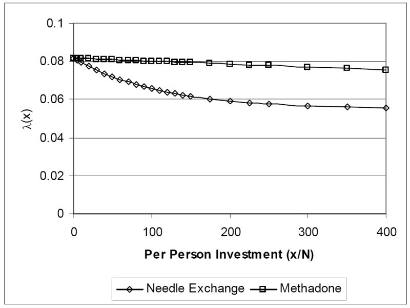
Estimated production functions for a needle exchange program (NEP) and a methadone maintenance treatment (MMT) program: sufficient contact rate λ(x) as a function of per person investment (x/N).

We modeled HIV transmission using an SI model with replacement [37]. This model has two disease states, susceptible and infected, denoted by S(t) and I(t). This model has three parameters: the fraction of the population that is infected at time zero (I(0), which corresponds to the initial disease prevalence), the replacement rate δ, and the sufficient contact rate λ. The population size is assumed to be constant (the total exit rate at any point in time equals the entry rate), and is denoted by N. The fraction of the population that is infected at time t (and thus the fraction of the population that is not infected) is given by the following equation:

$$I(t)=\{\begin{array}{ll}\frac{e^{(\lambda -\delta )t}}{\frac{\lambda (e^{(\lambda -\delta )t}-1)}{\lambda -\delta }+\frac{1}{I_0}}& \mathit{for}\lambda \ne \delta \\ \frac{1}{\lambda t+\frac{1}{I_0}}& \mathit{for}\lambda =\delta \end{array}$$ (6)

The function f(t,λ) is given by

$$\mathrm{f}(\mathrm{t},\lambda )=\text{λNI}(\mathrm{t})[1­\mathrm{I}(\mathrm{t})].$$ (7)

We calculated G(λ) as in equation (3) using T = 1 year (thus, 0 ≤ t ≤ 1) and an annual discount rate of r = 3%.

We first considered a stable epidemic with 40% HIV prevalence. This is similar to the prevalence seen among IDUs in areas such as New York City [38]. Zaric et al. [26] estimated a 3% non-HIV annual death rate among IDUs. We assumed survival of 12 years for untreated HIV [39] and 24 years for treated HIV [40], and that 75% of IDUs would eventually receive highly active antiretroviral treatment for HIV [41-43], leading to an average HIV-related life expectancy of 21 years. We thus assumed an annual death rate of.03+(1/21) = 7.76% among HIV-infected IDUs. Thus, the average death rate in the population (and therefore the replacement rate) is δ = .049 (=(.60×.03)+(.40×.0776)). The sufficient contact rate that corresponds to 40% HIV prevalence is calculated as λ₀ = (.049)/(.60) = .0817.

We calculated production functions of the form

$$\lambda (x)={\lambda }_{0}m(x).$$ (8)

We assume that the production function m(x) represents the behavior change achieved from one year of investment x in the program. When longer time horizons are considered, an investment would have to be made every year to maintain that level of behavior change.

Zaric and Brandeau [17] estimated the following production function for a needle exchange program based on data from the New Haven Legal Needle Exchange Program [13, 44]

$$m(x)=.67+.33e^{-.011\frac{x}{N}}$$ (9)

where N is the total population size. This was based on the estimate from the New Haven program that an expenditure of $65.22 per IDU yielded an overall reduction in needle sharing of 17.2%, and that the largest reduction in needle sharing that could be achieved would be 33% [13, 44]. With this function, an investment of $150,000 yields a risk multiplier of .950 in a population of 10,000. In 2006 dollars [45], the $150,000 cost is $191,000. Updating the production function to reflect 2006 dollars yields

$$m(x)=.67+.33e^{-.0089\frac{x}{N}}.$$ (10)

The corresponding production function (i.e., λ(x)=λ₀m(x)) has decreasing returns to scale (Figure 2).

For methadone maintenance, we estimated that for relatively small increases in capacity, benefits would be linear in investment [26]. Each methadone slot costs approximately $6494 (this value corresponds to $5250 in 1996 dollars [46], updated to 2006 dollars [45]), so (x/6494) is the number of new slots generated by an investment of x. Zaric et al. [26] estimated that the relative risk of infection for IDUs in methadone maintenance is 6% as high as that for IDUs not in methadone maintenance, so we estimated that each incremental slot would reduce overall transmission risk in the population by a multiplicative factor (.94/N). This yields the following function:

$$m(x)=1-\frac{.94x}{6494N}$$ (11)

The corresponding production function is linear (Figure 2). The maximum investment shown in Figure 2 corresponds to purchasing approximately 616 new methadone treatment slots (($400/person × 10,000 IDUs)/$6494/slot).

Figure 3 shows, for the needle exchange program and a time horizon of T = 1 year, the number of infections averted (top panel) as a function of per person investment, and the value of the objective function (bottom panel) as a function of per person investment for three values of W ($25,000, $50,000, and $100,000). The number of infections averted has decreasing returns to scale and the objective function is concave in the level of investment. Since the objective function is concave, the optimal solution is to either spend the entire budget or to spend up to the point x_D (which varies depending on W).

Figure 3.

Infections averted and objective function value for the needle exchange program, as a function of the net present value of investment, and for willingness-to-pay constant W = $25,000, $50,000, or $100,000 per HIV infection averted.

For example, consider the line corresponding to W = $50,000. The maximum value of W×IA(x)-x occurs at approximately x = $120 per person. If the budget is less than $120,000 (which corresponds to $120 per person), then it is optimal to spend the entire budget on the needle exchange program. If the budget is greater than $120,000, no more than $120,000 should be spent on the program; the rest of the funds should be spent on another intervention. Although additional funds would continue to avert infections (IA(x) is increasing in x), IA(x) has decreasing returns to scale. Thus, each additional unit of investment beyond $120,000 would yield benefits that are too small to justify the investment for that level of willingness to pay for benefits.

Figure 4 shows results for the methadone program. In this case, the number of infections averted (top panel) is approximately linear in the investment, as is the objective function (bottom panel). If the willingness to pay to avert a case of HIV is less than $300,000, then the objective function is negative for all levels of investment, and it is not optimal to invest in the methadone program. For a larger values of W, the objective function is positive and increasing in the amount invested, so it is optimal to invest the maximum amount possible in the methadone program.

Figure 4.

Infections averted and objective function value for the methadone program, as a function of the net present value of investment, and for willingness-to-pay constant W = $300,000, $400,000, or $500,000 per HIV infection averted.

For both programs, the value of the willingness-to-pay parameter (W) must be above a minimum level before any investment is made: this minimum value is approximately $20,000 per HIV infection averted for the needle exchange program and $300,000 for the methadone program.

The cases in Figures 3 and 4 correspond to the case of a stable epidemic, with 40% HIV prevalence among IDUs. Figure 5 shows the value of the objective function for the needle exchange program for different values of the sufficient contact rate, assuming W = $100,000. In the base case (λ = .0817), the optimal expenditure is approximately $200 per person when W = $100,000. For a smaller sufficient contact rate – and thus an epidemic that is shrinking below the initial 40% HIV prevalence – the optimal expenditure is lower: $75 per person if λ = .03 and $140 per person if λ = .05. For a larger sufficient contact rate than in the base case – and thus an epidemic that will grow above the initial 40% prevalence – the optimal expenditure is larger: approximately $250 per person if λ = .12. These results make intuitive sense: it is optimal to invest more in the prevention program when the epidemic is growing than when it is stable, and it is optimal to invest more when the epidemic is stable than when it is shrinking.

Figure 5.

Objective function value for the needle exchange program, for different values of the sufficient contact rate (λ₀ = .03, .05, .0817, and .12), assuming W = $100,000.

We also considered the case of a growing epidemic with 10% initial HIV prevalence among IDUs (and with δ= .049 and λ₀ = .0817 as in the base case above; thus, an epidemic with 10% prevalence that will grow to 40% prevalence). In this case, the willingness to pay to avert a case of HIV must be above $50,000 before any investment is made in the needle exchange program (Figure 6). For W = $100,000, the optimal expenditure on the needle exchange program is approximately $85 per person – an amount lower than the $200 per person spent when initial HIV prevalence is 40%.

Figure 6.

Objective function value for the needle exchange program, as a function of the net present value of investment, assuming a growing epidemic with initial HIV prevalence I(0) = .10 (with all other parameters the same as in the example of Figure 3), and for willingness-to-pay constant W = $100,000, $200,000, or $300,000 per HIV infection averted.

Finally, we considered a stable epidemic with 10% HIV prevalence among IDUs. This is similar to the prevalence seen among IDUs in areas such as San Francisco and Washington, DC [47, 48]. Using calculations similar to those above, we calculated epidemic parameters δ = . 0348 and λ ₀ = .0386 that lead to a stable epidemic with 10% prevalence. In this case (Figure 7), the willingness-to-pay constant must be higher than $100,000 per HIV case averted before any investment is made in needle exchange: for W = $200,000, the optimal investment is approximately $80/person.

Figure 7.

Objective function value for the needle exchange program, as a function of the net present value of investment, assuming a stable epidemic with initial HIV prevalence I(0) = .10 (with δ= .0348 and λ = .0386), and for willingness-to-pay constant W = $100,000, $200,000, or $300,000 per HIV infection averted.

For the lower prevalence population, a higher willingness to pay is required to justify investment compared to the higher prevalence population. Moreover, for any given value of W, the investment made in the lower prevalence population with a stable epidemic is less than the investment made in the lower prevalence population with a growing epidemic, which is less than the investment made in the higher prevalence population with a stable epidemic.

These examples underscore the need for decision makers to consider both the production function of the prevention program and the parameters of the epidemic when making decisions about how much to invest in an HIV prevention program.

5. Discussion

The optimal amount to spend on an HIV prevention program depends on the relationship between investment in the program and the resulting number of HIV infections averted. We have shown that this relationship can be expressed a function of the epidemic growth and of the prevention program’s production function. In general, the relationship between investment and HIV infections averted is not linear, so increased spending on a prevention program is not always cost effective. When infections averted has diminishing returns to scale in expenditure, it is optimal to invest only up to the point at which the marginal cost of the program equals its marginal benefit (expressed in terms of the willingness-to-pay factor W). When infections averted has increasing returns to scale in expenditure, it is optimal to either spend nothing or to spend the entire budget on the program.

In numerical analyses using a simple SI model, we found that the infections-averted function IA(x) tended to have the same returns-to-scale property as the production function λ(x) (although knowledge of both the production function and the epidemic growth is still required to determine the optimal level of expenditure). This highlights the importance of information about a prevention program’s production function. Brandeau et al. have provided guidelines for estimating basic information about such production functions [14]. To date, however, limited work has been done to estimate or infer production functions that directly link expenditure with reduction in HIV transmission risk [8, 13, 14, 16, 17, 21, 44]. For some programs, constant returns to scale have been estimated; other programs have been estimated to have decreasing returns to scale. A recent project assessing the efficiency of a variety of HIV prevention programs worldwide measured average program cost per unit of output (e.g., per person served) as a function of expenditure; this measure is likely a good surrogate for cost per reduction in transmission risk. The study found that some programs had decreasing returns to scale, whereas others had increasing and then decreasing returns to scale as expenditure increased [36]. An analysis of HIV prevention programs in Southern India that also measured cost per person served found increasing returns to scale in expenditure followed by decreasing returns to scale [35].

Our analysis has focused on optimal investment in a program aimed at preventing HIV, which is a communicable disease. For a non-communicable disease, epidemic effects are not relevant when considering the optimal level of investment in a prevention program, but the program’s production function is still relevant. Insights from studies that estimate production functions for non-communicable disease prevention programs could prove useful when estimating production functions for HIV prevention programs.

We have measured the health benefits of a prevention program in terms of HIV infections averted, but our analysis holds for any outcome measure that is a monotonically increasing function of total infections averted. For example, one could estimate quality-adjusted life years (QALYs) gained by multiplying the number of infections averted by an estimate of QALYs gained for each averted infection. Additionally, if one wished to use a range rather than a single value to define the acceptable cost-effectiveness threshold, our methodology could be used to find the corresponding range of expenditures.

Our model determines the optimal level of investment in a single HIV prevention program. When the decision maker must chose to invest in a single program from among competing prevention programs, the model can be used to determine the optimal amount to invest in each single program separately as we have done. The decision maker should then choose to invest in the program that averts the greatest number of infections at its optimal investment level. For the simple examples presented in Section 4, suppose the decision maker has a choice between needle exchange and methadone maintenance, a willingness to pay of W = $400,000 per HIV case averted, and a budget of $200 per person (net present value). In this case it is optimal when considering each program alone to spend the entire budget on that program. However, an investment of $200 per person on needle exchange averts approximately 54 HIV infections (Figure 3), whereas the same investment in the methadone program averts only 5 HIV infections (Figure 4). Thus, it is more cost effective (in terms of cost per HIV infection averted) to invest in the needle exchange program in this example. If the willingness to pay is $300,000 per HIV case averted, it would only make sense to invest in the needle exchange program (and it would be optimal to invest the maximum amount, $200 per person, on that program); at this level of willingness to pay, investment in the methadone maintenance program is not justified.

When the decision maker is choosing from among a portfolio of interventions that could be implemented simultaneously, a different model framework is needed (e.g., see [17, 18]) because the interventions may have interacting effects. For example, if both needle exchange and methadone maintenance are implemented, the number of infections averted is not the sum of the number that would be averted by each program alone because it is not possible to prevent the same infection twice. Moreover, as IDUs move into methadone maintenance, needle exchange may become less cost effective (because IDUs in methadone maintenance inject less often and share needles less often).

Our analysis has several limitations. We assumed that investment in a prevention program produces an instantaneous reduction in the sufficient contact rate. In practice, it is likely that such change is not instantaneous. A more sophisticated analysis could incorporate a non-constant sufficient contact rate. Additionally, our numerical analyses were based on a simple SI model with replacement. Depending on the population and intervention under consideration, other types of models, such as more sophisticated compartmental models [34, 49], network-based models [50], or discrete-event simulation models [12] could be used to more accurately capture epidemic effects when evaluating the likely impact of HIV prevention programs. For example, our illustrative analyses of investment in a needle exchange program and in a methadone program likely underestimate the benefits of these programs because the SI model does not capture sexual transmission of HIV from IDUs to non-IDUs. A more sophisticated model could capture this effect.

Despite these limitations, our work provides results that can be useful in making spending decisions. We have introduced a method for evaluating prevention program cost effectiveness for any feasible spending level, taking into account the characteristics of the epidemic and the prevention program. Natural next steps are the development of simple guidelines for decision makers as to how to characterize their local epidemic and how to understand the scale effects of prevention programs, and the incorporation of those guidelines into a simple planning tool that local decision makers could use when assessing potential investments in HIV prevention programs.

Appendix - Derivation of Optimal Expenditure Results in Table 1

Case 1: IA(x) has increasing returns to scale for 0 ≤ x ≤ B

If IA″(x) > 0, then IA(x) has increasing returns to scale. The optimal solution is specified as follows:

If W×IA(B) - B ≥ 0, then x* = B; otherwise, x* = 0.

Since IA(x) is increasing and has increasing returns to scale, the largest possible value of W×IA(x)-x will occur at the largest possible value of x, x=B. If this value is negative, then it must also be negative for all smaller values of x, x<B, and it is optimal to invest nothing. Note that if W×IA(B)-B=0, then a decision maker would be indifferent between investment of B versus none since the return on investment is exactly equal to the decision maker’s willingness to pay.

Case 2: IA(x) has decreasing returns to scale for 0 ≤ x ≤ B

If IA″(x) < 0, then IA(x) has decreasing returns to scale. We define the point x_D (if it exists) as the point that sets IA′(x_D)=1/W. The optimal solution is specified as follows:

1. If IA′(0) < 1/W, then x* = 0;

2. If x_D ≥ B, then x* = B;

3. If x_D < B, then x* = x_D.

In case (i), the benefits of investment are not justified by the costs even for the smallest possible investments. Since IA(x) has decreasing returns to scale, additional investments will yield proportionally fewer benefits, so it is optimal to invest nothing. In case (ii), the point at which marginal cost equals marginal benefit involves expenditure greater than available funds, so it is optimal to invest the entire budget. In case (iii), the point at which marginal cost equals marginal benefit involves an expenditure that is within the available budget, so it is optimal to invest up to this point. Since IA(x) has decreasing returns to scale, funds invested beyond x_D will generate less benefit than 1/W per dollar invested, and thus would represent wasted opportunities elsewhere.

Case 3: IA(x) has constant returns to scale for 0 ≤ x ≤B

If IA″(x) = 0, then IA(x) has constant returns to scale. The optimal solution is specified as follows:

If IA′(0) ≥ 1/W then x* = B; otherwise x* = 0.

In this case, if the marginal benefit of investment is greater than the marginal cost, it is worth investing the entire budget; otherwise, no investment should be made. If IA′(x)=1/W, a decision maker would be indifferent between investing anything in the intervention and not investing since the return on investment is exactly equal to the decision maker’s willingness to pay.

Case 4: IA(x) is “s-shaped” in the interval 0≤x≤B

Let x_F be a point of inflection (0 < x_F < B) where IA(x) switches from having increasing to decreasing returns to scale. IA(x) is “s-shaped” if IA″(x) > 0 for x < x_F and IA″(x) < 0 for x ≥ x_F. The optimal solution is determined by solving the two sub-problems corresponding to 0 ≤ x ≤ x_F (the region over which IA(x) has increasing returns to scale) and x_F < x ≤ B (the region over which IA(x) has decreasing returns to scale). The first problem is easily solved by comparing W×IA(x_F) - x_F and W×IA(0) - 0 = 0. The second problem is formed by defining λ₀=λ (x_F) and reducing the budget to B-x_F. The solution to the second problem will indicate whether any additional investment beyond x_F is required. The solution to this second problem is found using the methods outlined above for the case of decreasing returns to scale.

References

- 1.World Health Organization. Global HIV prevalence has levelled off. [March 7, 2008];2007 Available at http://www.who.int/mediacentre/news/releases/2007/pr61/en/index.html.
- 2.Joint United Nations Programme on HIV/AIDS (UNAIDS) Resource needs for an expanded response to AIDS in low- and middle-income countries. [March 7, 2008];2005 Available at http://www.unaids.org/html/pub/publications/irc-pub06/resourceneedsreport_24jun05_en_pdf.pdf.
- 3.Earnshaw SR, Hicks K, Richter A, et al. A linear programming model for allocating HIV prevention funds with state agencies: a pilot study. Health Care Manage Sci. 2007;10(3):239–252. doi: 10.1007/s10729-007-9017-8. [DOI] [PubMed] [Google Scholar]
- 4.Ruiz M, Gable A, Kaplan EH, et al., editors. No time to lose: getting more from HIV prevention. National Academy Press; Washington, DC: 2001. [PubMed] [Google Scholar]
- 5.Holtgrave DR, Kelly JA. Preventing HIV/AIDS among high-risk urban women: the cost-effectiveness of a behavioral group intervention. Am J Public Health. 1996;86:1442–1445. doi: 10.2105/ajph.86.10.1442. [DOI] [PMC free article] [PubMed] [Google Scholar]
- 6.Pinkerton SD, Holtgrave DR, Di Franceisco WJ, et al. Cost effectiveness of a community-level HIV risk reduction intervention. Am J Public Health. 1998;88:1239–1242. doi: 10.2105/ajph.88.8.1239. [DOI] [PMC free article] [PubMed] [Google Scholar]
- 7.Kahn JG, Kegeles SM, Hays R, et al. The cost-effectiveness of the Mpowerment Project, a community-level intervention for young gay men. J Acquir Immune Defic Syndr. 2001;27(5):482–491. doi: 10.1097/00126334-200108150-00010. [DOI] [PubMed] [Google Scholar]
- 8.Dandona L, Sisodia P, Kumar SG, et al. HIV prevention programmes for female sex workers in Andhra Pradesh, India: outputs, cost and efficiency. BMC Public Health. 2005 Sep 24;5:98. doi: 10.1186/1471-2458-5-98. [DOI] [PMC free article] [PubMed] [Google Scholar]
- 9.Heumann KS, Marx R, Lawrence SJ, et al. Cost-effectiveness of prevention referrals for high-risk HIV negatives in San Francisco. AIDS Care. 2001;13:637–642. doi: 10.1080/09540120120063269. [DOI] [PubMed] [Google Scholar]
- 10.Pinkerton SD, Holtgrave DR, Valdiserri RO. Cost-effectiveness of HIV-prevention skills training for men who have sex with men. AIDS. 1997;11(3):347–357. doi: 10.1097/00002030-199703110-00013. [DOI] [PubMed] [Google Scholar]
- 11.Ratcliffe J, Ades AE, Gibb D, et al. Prevention of mother-to-child transmission of HIV-1 infection: alternative strategies and their cost effectiveness. AIDS. 1998;12(11):1381–1388. doi: 10.1097/00002030-199811000-00021. [DOI] [PubMed] [Google Scholar]
- 12.Rauner MS, Brailsford SC, Flessa S. Use of discrete-event simulation to evaluate strategies for the prevention of mother-to-child transmission of HIV in developing countries. J Operational Res Soc. 2005;56(2):222–233. [Google Scholar]
- 13.Kaplan EH. Economic analysis of needle exchange. AIDS. 1995;9(10):1113–1119. doi: 10.1097/00002030-199510000-00001. [DOI] [PubMed] [Google Scholar]
- 14.Brandeau ML, Zaric GS, de Angelis V. Improved allocation of HIV prevention resources: using information about program effectiveness. Health Care Manage Sci. 2005;8(1):19–28. doi: 10.1007/s10729-005-5213-6. [DOI] [PubMed] [Google Scholar]
- 15.Brandeau ML, Zaric GS, Richter A. Optimal resource allocation for epidemic control among multiple independent populations: beyond cost effectiveness analysis. J Health Econ. 2003;22(4):575–598. doi: 10.1016/S0167-6296(03)00043-2. [DOI] [PubMed] [Google Scholar]
- 16.Richter A, Brandeau ML, Owens DK. An analysis of optimal resource allocation for prevention of infection with human immunodeficiency virus (HIV) in injection drug users and non-users. Med Decis Making. 1999;19(2):167–179. doi: 10.1177/0272989X9901900207. [DOI] [PubMed] [Google Scholar]
- 17.Zaric GS, Brandeau ML. Optimal investment in a portfolio of HIV prevention programs. Med Decis Making. 2001;21(5):391–408. doi: 10.1177/0272989X0102100506. [DOI] [PubMed] [Google Scholar]
- 18.Zaric GS, Brandeau ML. Resource allocation for epidemic control over short time horizons. Math Biosci. 2001;171(1):33–58. doi: 10.1016/s0025-5564(01)00050-5. [DOI] [PubMed] [Google Scholar]
- 19.Zaric GS, Brandeau ML. A little planning goes a long way: multi-level allocation of HIV prevention resources. Med Decis Making. 2007;27(1):71–81. doi: 10.1177/0272989X06297395. [DOI] [PubMed] [Google Scholar]
- 20.Kaplan EH, Pollack H. Allocating HIV prevention resources. Socio-Econ Plann Sci. 1998;32(4):257–263. [Google Scholar]
- 21.Kaplan EH. Economic evaluation and HIV prevention community planning. A policy analyst’s perspective. In: Holtgrave DR, editor. Handbook of HIV prevention policy analysis. Plenum Press; New York: 1998. pp. 177–193. [Google Scholar]
- 22.Friedrich CM, Brandeau ML. Using simulation to find optimal funding levels for HIV prevention programs with different costs and effectiveness. In: Katzper M, Anderson JG, editors. Proceedings of the 1998 Medical Sciences Simulation Conference. The Society for Computer Simulation International; San Diego. 1998. pp. 58–64. [Google Scholar]
- 23.Holtgrave DR, Qualls NL. Threshold analysis and programs for prevention of HIV infection. Med Decis Making. 1995;15(4):311–317. doi: 10.1177/0272989X9501500402. [DOI] [PubMed] [Google Scholar]
- 24.Sanders GD, Bayoumi AM, Sundaram V, et al. Cost effectiveness of screening for HIV in the era of highly active antiretroviral therapy. N Engl J Med. 2005;352(6):32–47. doi: 10.1056/NEJMsa042657. [DOI] [PubMed] [Google Scholar]
- 25.Walensky RP, Weinstein MC, Kimmel AD, et al. Routine HIV testing: an economic evaluation of current guidelines. Am J Med. 2005;118(3):292–300. doi: 10.1016/j.amjmed.2004.07.055. [DOI] [PubMed] [Google Scholar]
- 26.Zaric GS, Barnett PG, Brandeau ML. HIV transmission and the cost effectiveness of methadone maintenance. Am J Public Health. 2000;90(7):1100–1111. doi: 10.2105/ajph.90.7.1100. [DOI] [PMC free article] [PubMed] [Google Scholar]
- 27.Armbruster B, Brandeau ML. Optimal mix of screening and contact tracing for endemic diseases. Math Biosci. 2007;209(2):386–402. doi: 10.1016/j.mbs.2007.02.007. [DOI] [PMC free article] [PubMed] [Google Scholar]
- 28.Kahn JG, Marseille E, Auvert B. Cost effectiveness of male circumcision for HIV prevention in a South African setting. PLoS Medicine. 2006;3(12):2349–2358. doi: 10.1371/journal.pmed.0030517. [DOI] [PMC free article] [PubMed] [Google Scholar]
- 29.Goldie SJ, Paltiel AD, Weinstein MC, et al. Projecting the cost-effectiveness of adherence interventions in persons with human immunodeficiency virus infection. Am J Med. 2003;115(8):632–641. doi: 10.1016/j.amjmed.2003.07.007. [DOI] [PubMed] [Google Scholar]
- 30.Owens DK. Interpretation of cost-effectiveness analyses [Editorial] J Gen Intern Med. 1998;13:716–717. doi: 10.1046/j.1525-1497.1998.00211.x. [DOI] [PMC free article] [PubMed] [Google Scholar]
- 31.World Health Organization. The world health report 2002 - reducing risks, promoting healthy life. World Health Organization; Geneva, Switzerland: 2002. [Google Scholar]
- 32.Herbst JH, Sherba RT, Crepaz N, et al. A meta-analytic review of HIV behavioral interventions for reducing sexual risk behavior of men who have sex with men. J Acquir Immune Defic Syndr. 2005;39(2):228–241. [PubMed] [Google Scholar]
- 33.Kaplan EH. Needles that kill: modeling human immunodeficiency virus transmission via shared drug injection equipment in shooting galleries. Rev Infect Dis. 1989;11(2):289–298. doi: 10.1093/clinids/11.2.289. published erratum appears in Rev Infect Dis 1989 Jul-Aug;11(4):672. [DOI] [PubMed] [Google Scholar]
- 34.Zaric GS, Brandeau ML, Barnett PG. Methadone maintenance and HIV prevention: a cost effectiveness analysis. Manage Sci. 2000;46(8):1013–1031. [Google Scholar]
- 35.Guinness L, Kumaranayake L, Hanson K. A cost function for HIV prevention services: is there a ’u’ -shape? Cost Eff Resour Alloc. 2007 Nov 5;5:13. doi: 10.1186/1478-7547-5-13. [DOI] [PMC free article] [PubMed] [Google Scholar]
- 36.Marseille E, Dandona L, Marshall N, et al. HIV prevention costs and program scale: data from the PANCEA project in five low and middle-income countries. BMC Health Serv Res. 2007 Jul 12;7:108. doi: 10.1186/1472-6963-7-108. [DOI] [PMC free article] [PubMed] [Google Scholar]
- 37.Bailey NTJ. The mathematical theory of infectious diseases and its applications. Hafner Press; New York: 1975. [Google Scholar]
- 38.Des Jarlais DC, Friedman SR, Sotheran JL, et al. Continuity and change within an HIV epidemic. Injecting drug users in New York City, 1984 through 1992. JAMA. 1994;271(2):121–127. [PubMed] [Google Scholar]
- 39.Longini IM, Clark WS, Byers RH, et al. Statistical analysis of the stages of HIV infection using a Markov model. Stat Med. 1989;8(7):831–843. doi: 10.1002/sim.4780080708. [DOI] [PubMed] [Google Scholar]
- 40.Schackman BR, Gebo KA, Walensky RP, et al. The lifetime cost of current human immunodeficiency virus care in the United States. Med Care. 2006;44(11):990–997. doi: 10.1097/01.mlr.0000228021.89490.2a. [DOI] [PubMed] [Google Scholar]
- 41.Altice FL, Maru DS, Bruce RD, et al. Superiority of directly administered antiretroviral therapy over self-administered therapy among HIV-infected drug users: a prospective, randomized, controlled trial. Clin Infect Dis. 2007;45(6):770–8. doi: 10.1086/521166. [DOI] [PMC free article] [PubMed] [Google Scholar]
- 42.Lucas GM, Weidle PJ, Hader S, et al. Directly administered antiretroviral therapy in an urban methadone maintenance clinic: a nonrandomized comparative study. Clin Infect Dis. 2004;38(Suppl 5):S409–S413. doi: 10.1086/421405. [DOI] [PubMed] [Google Scholar]
- 43.Lucas GM, Mullen BA, Weidle PJ, et al. Directly administered antiretroviral therapy in methadone clinics is associated with improved HIV treatment outcomes, compared with outcomes among concurrent comparison groups. Clin Infect Dis. 2006;42(11):1628–1635. doi: 10.1086/503905. [DOI] [PubMed] [Google Scholar]
- 44.Kaplan EH, O’Keefe E. Let the needles do the talking! Evaluating the New Haven needle exchange. Interfaces. 1993;23(1):7–26. [Google Scholar]
- 45.National Aeronautics and Space Administration. GDP inflation calculator. [March 7, 2008];2007 Available at http://cost.jsc.nasa.gov/inflateGDP.html.
- 46.Barnett PG. The cost-effectiveness of methadone maintenance as a health care intervention. Addiction. 1999;94(4):479–488. doi: 10.1046/j.1360-0443.1999.9444793.x. [DOI] [PubMed] [Google Scholar]
- 47.Moss AR, Vranizan K, Gorter R, et al. HIV seroconversion in intravenous drug users in San Francisco, 1985-1990. AIDS. 1994;8(2):223–231. doi: 10.1097/00002030-199402000-00010. [DOI] [PubMed] [Google Scholar]
- 48.Friedman SR, Lieb S, Tempalski B, et al. HIV among injection drug users in large U.S. metropolitan areas, 1998. J Urban Health. 2005;82(3):434–445. doi: 10.1093/jurban/jti088. [DOI] [PMC free article] [PubMed] [Google Scholar]
- 49.Long EF, Brandeau ML, Galvin CM, et al. Slowing the HIV epidemic in St. Petersburg, Russia: effectiveness and cost-effectiveness of expanded antiretroviral therapy. AIDS. 2006;20(17):2207–2215. doi: 10.1097/QAD.0b013e328010c7d0. [DOI] [PubMed] [Google Scholar]
- 50.Armbruster B, Brandeau ML. Contact tracing to control infectious disease: when enough is enough. Health Care Manage Sci. 2007;10(4):341–355. doi: 10.1007/s10729-007-9027-6. [DOI] [PMC free article] [PubMed] [Google Scholar]