Repeated Measurements on Distinct Scales With Censoring—A Bayesian Approach Applied to Microarray Analysis of Maize

Abstract

We analyze data collected in a somatic embryogenesis experiment carried out on Zea mays at Iowa State University. The main objective of the study was to identify the set of genes in maize that actively participate in embryo development. Embryo tissue was sampled and analyzed at various time periods and under different mediums and light conditions. As is the case in many microarray experiments, the operator scanned each slide multiple times to find the slide-specific ‘optimal’ laser and sensor settings. The multiple readings of each slide are repeated measurements on different scales with differing censoring; they cannot be considered to be replicate measurements in the traditional sense. Yet it has been shown that the choice of reading can have an impact on genetic inference. We propose a hierarchical modeling approach to estimating gene expression that combines all available readings on each spot and accounts for censoring in the observed values. We assess the statistical properties of the proposed expression estimates using a simulation experiment. As expected, combining all available scans using an approach with good statistical properties results in expression estimates with noticeably lower bias and root mean squared error relative to other approaches that have been proposed in the literature. Inferences drawn from the somatic embryogenesis experiment, which motivated this work changed drastically when data were analyzed using the standard approaches or using the methodology we propose.

1. INTRODUCTION—AN EXPERIMENT TO ASSESS GENE EXPRESSION CHANGES DURING MAIZE EMBRYOGENESIS

Somatic embryogenesis in Zea mays is an important tool for genetic engineering. Natural plant development from a fertilized egg cell follows zygotic embryogenesis into a seed and eventually a mature plant. Somatic embryos begin as callus (undifferentiated cells) and are induced to develop into embryos by immersion in an embryogenic medium. Callus can be generated from existing plants by transfer to a callus-generating medium. Mature plants can then be grown from existing plant material through organogenesis, but this skips the embryonic stage. Somatic embryogenesis creates embryos that are similar to those arising from sexual reproduction and which have the same genotype as the explant from which they were created.

The first somatic embryos in maize tissue culture were produced by Green and Phillips (1975). Armstrong and Green (1985) found that cell lines derived from sources such as immature embryos are heterogeneous for cells with different embryogenic competence and that certain types of callus tend to be more embryogenic. Unfortunately, embryogenic competence is genotype-specific in many plant species including Zea mays, and often the most desirable or economically important lines are difficult to induce to regeneration. Because genetic transformation of the plant in the embryonic stage has enormous potential for development of high yielding varieties, it is important to recognize embryonic cells or tissues and to identify markers for them. In this way we hope to develop tools for improving embryogenic competence in particular maize lines.

To identify the genetic traits responsible for highly embryogenic lines, we examined gene expression changes during maize somatic embryo development. Somatic embryos were generated in six embryogenic callus lines (labeled A, B, C, D, E, and F) developed from immature Hi II embryo explants. These lines are assumed to be random samples from the population of Hi II lines. Hi II is a regeneration-proficient hybrid of Zea mays, which also produces high crop yields and thus is of economic importance. After callus populations were generated from the six lines in a callus-generating medium (N6E medium þ2, 4-D, 3% sucrose), embryogenic calli (identifiable by shape) were selected from the total callus for each of the lines. These selected calli were matured into somatic embryos by transferring them to a sucrose-enhanced medium (Regen Medium I -2, 4-D, 6% sucrose). After 21 days in the dark, the embryos were exposed to light and transferred to a new medium (Regen Medium II -2, 4-D, 3% sucrose) to encourage germination. Material was sampled at five time points during the development and maturation of the embryos into seedlings; see Figure 1.

Figure 1.

The time course experiment for somatic embryogenesis in maize.

The material used in the microarray analysis comes from the pooled pair of lines rather than from individual plant lines. Pools were labeled AB, CD, and EF. Gene expression patterns in the AB, CD and EF lines were profiled using 12,060 element maize cDNA arrays. The experimental design was a loop design with dye-swapping for line pools AB, CD, and EF, which resulted in a total of 30 slides. Under our design, gene expression is measured at each time point four times within each line pool, so that across line pools, time point samples are repeated 12 times. Not all replicates are independent, however, because the four technical replicates within a line pool used the same biological material. The design therefore allows for an analysis of the measurement variance across time and across line pools. For details on the microarray design considerations, see the Appendix A.4. The dataset used in this analysis can be obtained by contacting the authors.

We are interested in identifying the genes or groups of genes that actively participate in somatic embryogenesis. These genes will exhibit significant changes in their expression over the course of tissue development and maturation. Whereas most of the genes participating in embryonic development are expected to be up-regulated as embryos mature, it is also possible that some genes active in embryogenesis will downregulate over time or will exhibit some other expression profiles. Therefore, we seek to classify the 12,060 elements of the microarrays into those with constant expression over all time points and those with any other pattern of expression. Some initial results obtained using a subset of these data and standard statistical methods are reported in Che et al. (2004), however our collaborators in Plant Science had anticipated a more extensive group of differentially expressed genes and inspired development of our methods here.

As is often the case in microarray experiments, each slide was scanned multiple times using different laser and sensor settings. By varying the settings of the instruments, the operator can strike a balance between over-exposing the highly expressing genes while still picking up a signal from the lowly fluorescing spots. In a typical statistical analysis of gene expression data, only the “best” scan of each slide is included in the analysis and the rest are discarded (Swanson-Wagner et al. 2006). Yet it has been argued (Romualdi, Trevisan, Celegato, Costa, and Lanfranchi 2003; Lyng et al. 2004; Skibbe et al. 2006) that different choices by the operator can have an impact on the set of genes identified as differentially expressed.

We propose an approach that permits estimating gene expression profiles using all available measurements for each spot. We show that by making use of the additional information we obtain estimates of quantities of interest that are better (in the minimum mean squared error (MSE)-sense) than all other approaches recently reported in the literature. Importantly, the set of genes identified as possibly embryogenic in our experiment changes if all scans, rather than just the best, are used in statistical analyses of the data and the new set of genes is more biologically plausible than the old one.

This article is organized as follows. In Section 2 we provide some background on the cDNA microarray technology and include a discussion on the effects of changing laser and sensor settings on the readings obtained for a slide. We propose a new method for estimating gene expression profiles using multiple array scans in Section 3. The performance of the approach is compared with that of other approaches proposed in the literature via simulation in Section 4. We finally revisit the original embryogenesis study and analyze the experimental data using the standard and the proposed approaches. Results are presented in Section 5 and discussed in Section 6. Details on some of the derivations presented in the article and the specifics of standard microarray analysis methods used are given in an Appendix.

2. MICROARRAY ANALYSIS

The data generated from microarray experiments are obtained from images of the microarray slides. These images come from the scanner and record the intensity of fluorescence on the slide. The analysis of microarray data generates conclusions from these images through the following five stages of analysis:

1. Spot finding and background correction

2. Generating one intensity estimate per slide channel from multiple scans

3. Normalization across slides to make them comparable

4. Identification of differentially expressed genes

5. Post hoc analysis of differentially expressed genes (for example, by clustering)

The ordering of the first two steps is flexible under special circumstances of data collection. For instance, Romualdi et al. (2003) combine multiple scans at the pixel level before finding spots because all scans had identical settings. Generally, the scan to be used is selected by eye and thus before segmentation and background correction. Additionally, if there is only one scan, then the second stage is trivial.

The data generated from cDNA microarray experiments consist of two types of images of the microarray slide. The two images are obtained while the slide is excited with a laser tuned to Cy5 and to Cy3 fluorescent dyes, respectively, to match the dyes of the two biological samples applied to each slide. Different laser strengths and the sensitivities of the camera result in different images. Where as a particular setting for laser and camera may produce a large number of saturated spots on the slide image, other settings may result in too many spots with measured expression below the minimum that can be captured by the instruments. The laser strength and the sensitivity of the photomultiplier to light are generally adjusted by the operator to produce several scans of the microarray. The operator may find a ‘best’ picture, such as one where most of the spots show some measurable expression and where very few of the spots reach saturation and only send that image on for analysis. This is the standard approach to stage 2 analysis of microarrays (see Swanson-Wagner et al. (2006) for one of very few mentions of this practice in the literature).

In this work, we focus on the second stage of microarray analysis and the measurement error that is introduced when scientists vary the strength of the laser and the sensitivity of the photomultiplier used to amplify the expression signals and propose a modeling approach that allows incorporating multiple readings of each slide into the analysis. We show that under relatively lax model assumptions, expression levels can be estimated with significantly lower bias and higher precision when combining multiple readings for each gene into the statistical analysis than when choosing only the ‘best’ reading. For all other stages of analysis (spot selection, background cleaning, normalization, and identification of differential expression) we use standard techniques (see Appendix A.5 for more details).

Methods for estimating gene expression that use the multiple slide scans that are typically produced in microarray experiments have been discussed in the literature in recent years. Lyng et al. (2004) and Skibbe, Nettleton, and Schnable (2006) investigated the effects of scanner settings on expression ratios and significant differential expression, respectively. Both found that scanner settings have an important impact on the quality of and conclusions from microarray data. Lyng et al. (2004) suggests using two scans at different settings to increase the usable range of expression values. Romualdi et al. (2003) suggest combining the pixel intensities over multiple slide readings by averaging them before segmentation to create more uniform spots. However, the same scanner settings must be used to make the pixels exchangeable between scans. This means that there was no improvement of the dynamic range of expression estimates by Romualdi et al. (2003). Dudley, Aach, Steffen, and Church (2002) and Garcia de la Nava, van Hijum, and Trelles (2004) used multiple slide readings at varying settings to extend the dynamic range and address the censoring error. However, the former used only the estimate from one reading for each gene (possibly linearly transformed) whereas the latter accommodated only two scans. Thus, whereas the challenges that arise when attempting to use all measurements of a slide in statistical analyses have been recognized, no fully satisfactory approach has yet been proposed.

Most work on microarray analysis has addressed the problem of finding differentially expressed genes (what we have labeled as stage 4 in the analysis) although all stages have received some attention in the literature. In recent years, hierarchical models have been developed to identify differentially expressed genes over two or more treatments and with or without biological and technical replicates (including Newton, Kendziorski, Richmond, Blattner, and Tsui (2001) and Kendziorski, Newton, Lan, and Gould (2003)). These models use mixtures of differentially expressed and equivalently expressed genes to estimate the posterior probability of differential expression and the proportion of differentially expressed genes in an experiment. Whereas these models use the same distributions as our models, they do not address the replication of microarray scans on different scales because they assume that normalization has already been performed on all replicates to place them on the same scale. Those models cannot be trivially extended to unnormalized replicates on varied scales. Alternatively, each scan could be normalized separately and counted as a different technical replicate. However, it is unclear how one might proceed with normalization under this approach because there is no longer a pairing of observations sharing a slide that can be used to remove the intensity-dependent dye bias.

Doubly-censored models and other methods for treating the limited range of values obtained from the microarray scanners have also received some attention. As mentioned, Dudley et al. (2002) extends the usable range of expression values by linearly extrapolating between multiple scans without explicitly modeling the observed data as censored. Wit and McClure (2003) develop adjustments to expression estimates based on the approximate linear relationship between spot pixel mean, median, and standard deviation for uncensored spots, again without modeling censoring explicitly. Tadesse, Ibrahim, and Mutter (2003) model expression values from oligonucleotide arrays as doubly-censored with a lognormal likelihood after normalization without using multiple scans. We propose that after normalization, censoring has been further complicated by the transformation and therefore, modeling censoring on the original scale is more appropriate.

2.1 Multiple Laser and Sensor Settings

Different laser and sensor settings can be used to read a cDNA microarray slide. Stronger laser settings create more fluorescence and stronger sensor settings pick up more signal. There is a balance to be struck between picking up signal from the lowly fluorescing spots and over-exposing the highly expressing genes. There is an upper limit to the measurement of fluorescence (most often 65,535 = 2¹⁶ − 1 due to the limit of double precision memory, which allows 2¹⁶ distinct values); readings of spots that are brighter are censored. Over-exposing the high intensity spots will cause them to be artificially near other high expression values. Correspondingly, low signals will be artificially assigned to 0 if the laser and sensor settings are too low.

Figure 2 illustrates the two scenarios. It is possible to have both overexposed and underexposed spots in the same scan. The expression estimates used are background corrected average pixel intensities (see Appendix A.5 for details). Any spot will have variation in its pixels due to inconsistencies in spot printing and irregular spot shape. Further, background correction will reduce the measured expression value so that 65,535 is no longer the point of censoring (see Fig. 2 (a) where there is censoring at around 50,000) and create expression estimates that are negative or near zero. Negative expression measurements are routinely set to zero, however, often the true point of censoring is not zero (see Fig. 2 (b) where there is censoring near 10).

Figure 2.

(a) Many spots are censored above in the higher reading. (b) Many spots are censored below in the lower reading.

Multiple readings of the microarray slides can be taken for both fluorescence channels. Because all of the readings at different settings attempt to capture true expression levels for the genes on the slide, it is reasonable to assume that all readings contribute useful information about true expression levels and to think of combining the multiple readings into one estimate of gene expression for each spot. If the readings at different settings contain information about the true expression of the gene, then the variance in estimated gene expression that is due to the measurement process should be reduced in estimates based on all available readings.

Several aspects of the measurement process of gene expression create challenges for statistical modeling. As discussed earlier, many microarray experiments include pseudo-replicates, which we define as multiple readings of the slide under different laser and sensor settings. Generally, settings for different slides are very different because of the large experimental variation between slides. That is, one slide may result in a good reading at low laser and sensor settings whereas another may require higher settings to reduce the number of expression levels below the threshold while keeping the number of overexposed spots to a minimum. Because of this practice, we are typically unable to assume that the settings act as blocks in a traditional experimental design. However, because the settings to read the two channels are almost always chosen independently across slides, we can model each slide/ dye combination separately. In what follows, we consider an arbitrary slide and dye channel in the experiment and propose a hierarchical model for estimating gene expression levels that permits incorporating multiple measurements for each gene into a single analysis.

3. BAYESIAN HIERARCHICAL GAMMA MODEL

To estimate gene expression, we propose a Bayesian hierarchical model. The approach we propose is only similar to the one proposed in Newton et al. (2001) and Kendziorski et al. (2003) in that it assumes that gene expression can be represented using a Gamma probability model. The fact that we describe a model to account for all measurements of a slide (potentially collected at different instrument settings) results in a significantly different formulation for the statistical model in almost all other aspects. This model incorporates all slide scans into one estimate of expression per spot. Also of significance is that the modeling is done on each slide separately. The estimates generated are only later compared across slides to identify differential expression in further analysis, so that concerns about correlations across genes on a slide are not present at this level.

To formulate the model, we rely on the natural ordering of slide readings. For instance, if we have two readings with the same sensor setting and different laser settings, the measurements on the reading with the higher laser setting will tend to be larger. Dudley et al. (2002) discuss gene expression and its dependence on changes in one of the experimental settings (laser or sensor). Here we consider changing multiple settings simultaneously so that there is not an obvious ordering based on level of the settings; one setting may be raised and the other lowered. Using the fact that the scans will still be naturally ordered, we use median readings to order the slides from smallest to largest. Clearly, the median-based ordering is robust to censoring but subject to some uncertainty due to the measurement error in observed gene expressions. However, this is of no concern because ordering is done merely as a conceptual convenience and is not essential to the model.

3.1 Likelihood Function

Suppose that there are m + 1 readings taken on n spots on a particular slide and dye combination. In the maize embryogenesis experiment, m + 1 = 3 and n = 12,060 for each of the 60 slide/dye combinations, but the number of readings need not be constant over slides because they are analyzed separately. In the following we consider one arbitrary slide and dye channel in the experiment and therefore do not include the indexes of slide and dye. For a given gene i, we use S_i1, …, S_i(m+1) to denote the m + 1 signal measurements. Here S_i1 is the gene expression measurement from the scan having the smallest median expression (of all spots on the scan) and S_i(m+1) denotes the reading for gene i on the scan with the highest median expression. However, S_i1 ≤ … ≤ S_i(m+1) is not true for each i. This is because the ordering is done on the scans, not on each spot; measurement error for each scan can cause S_i′1 > S_i′2 though S_i1 < S_i2 for most spots (i).

We assume that all readings measure the same quantity—actual gene expression—with error. Therefore, under suitable scaling the readings would be identically distributed. We assume that the scaled readings (which are strictly positive) can be represented by a Gamma distribution. The Gamma has support on the positive real line and, depending on parameter values, exhibits noticeable skewness. (This model has also been implemented with a lognormal likelihood and the derivation is along the same lines.) Therefore, in the absence of censoring, we could model the signals for each gene i across the m + 1 readings in the following way:

$$S_{ij}*{\chi }_j=S_{ij}^{\prime }\sim \mathrm{\Gamma }(a,{\psi }_i)$$

for all i = 1, …, n and j = 1, …, m + 1, where the χ_j are constant for all genes in a given slide/dye combination. Here, the $S_{ij}^{\prime }$ are the appropriately scaled expression values (which are conditionally independent given the gene specific scale parameters ψ_i) and the χ_j are the scaling factors that adjust the observed expression values to the correct scale. This assumes that the changes in laser and sensor settings increase or decrease each spot’s fluorescence by the same multiplicative factor. This assumption appears reasonable based on exploratory analysis, equipment specifications, and other papers (Wit and McClure 2003). This model can also be written as

$$S_{ij}\sim \mathrm{\Gamma }(a,{\psi }_i{\chi }_j)$$

for all i = 1, …, n and j = 1, …, m + 1.

As formulated, the likelihood is not identifiable (as shown in Appendix 8.1), in that there is no way to estimate the parameters, a, ψ, and χ, directly. Thus, we do not attempt to estimate ψ_i and instead focus on estimating θ_i = χ_m+1ψ_i. Of course, using proper priors on our parameters, as we shall, it is not necessary to have an identifiable likelihood. However, both the ψ and χ are relative values (of gene expression and fluorescence scaling) and the χ are nuisance parameters. Additionally, the negative correlation between the average ψ_i estimate and the average χ_j estimate makes estimating these parameters with sequential sampling methods difficult.

We choose the highest of the m + 1 readings as a reference reading and scale all other readings to that level, though any of the readings could be chosen for the reference level. By scaling all readings upwards to the highest one we are increasing the effective range of gene expression measurement. This does not limit the usefulness of the model in any way, because all measures of gene expression are relative and normalization is subsequently performed on the expression estimates. Additionally, we do not restrict ψ_iχ₁ ≤ … ≤ ψ_iχ_m+1, though this is our conceptual framework. Such ordering would be a very strong assumption and rely on the ordering of the scans using the medians. Instead, we use a more general model that does not use the ordering of the scans for anything except picking the reference (observed highest) scan. This also allows our model to be used in its present form with a different reference scan.

We now have the following model, still assuming that no censoring occurs:

$$S_{ij}\sim \mathrm{\Gamma }(a,{\theta }_i{\delta }_j)$$

for all i = 1, …, n and j = 1, …, m + 1, where δ_j are constant for all genes in a given slide and dye combination and δ_m+1 ≡ 1. Here, the δ_j are the scaling factors that adjust the observed expression values to the reference scale. We let S = {S_ij} denote the set of measurements on a particular slide and dye. The unknown parameters in this model are a, θ₁, …, θ_n, and δ₁, …, δ_m.

This likelihood model assumes that we observe all the values of S_ij. Yet we do not observe intensity of spots in readings where they are censored; however, we do know that they are censored above (below) and that the measurement is larger (smaller) than a known value. We define an indicator variable, C_ij, where C_ij = 0 if observation S_ij is not censored, C_ij = 1 if observation S_ij is censored below, and C_ij = 2 if observation S_ij is censored above. This variable and the subset of S,S^(o),which includes noncensored measurements make up our observed data. The measurements that would have been observed in the absence of censoring are therefore taken to be missing. The set of missing data are denoted by S^(m) and S = S^(o) ∪ S^(m). In a Bayesian framework, we can estimate missing values along with parameters.

In practice a spot can be designated as censored below if any of its pixels are less than the background value. A spot can be designated as censored above if any of its pixels are saturated. Alternatively, exploratory data analysis can be used to decide appropriate cut-off values for a particular slide/dye combination, such as 5 and 50,000. For these threshold values, the maize embryogenesis experiment has 2,337 genes, which are censored below on at least one of the 60 measurements and 322 genes, which are censored above on at least one measurement. We shall denote the lower and upper truncation points by L and U, respectively.

We now examine the conditional likelihood of S_ij, given the censoring indicator, C_ij. Let f(·|λ) be the density function of the Gamma(a, λ) distribution and F(·|λ) be its cumulative distribution function. Then double censoring implies that the joint probability of S_ij and C_ij can be written in the following form:

$$\begin{array}{cc}p(S_{ij},C_{ij}|{\theta }_i{\delta }_j)\hfill & =p(S_{ij}|C_{ij}=0,{\theta }_i{\delta }_j)p(C_{ij}=0|{\theta }_i{\delta }_j)\hfill \\ \hfill & +p(S_{ij}|C_{ij}=1,{\theta }_i{\delta }_j)p(C_{ij}=1|{\theta }_i{\delta }_j)\hfill \\ \hfill & +p(S_{ij}|C_{ij}=2,{\theta }_i{\delta }_j)p(C_{ij}=2|{\theta }_i{\delta }_j)\hfill \\ \hfill & =f(S_{ij}|{\theta }_i{\delta }_j)I_{(L,U)}(S_{ij})I_{\{0\}}(C_{ij})\hfill \\ \hfill & +f(S_{ij}|{\theta }_i{\delta }_j)I_{(0,L]}(S_{ij})I_{\{1\}}(C_{ij})\hfill \\ \hfill & +f(S_{ij}|{\theta }_i{\delta }_j)I_{[U,\infty )}(S_{ij})I_{\{2\}}(C_{ij}).\hfill \end{array}$$ (1)

We shall divide the set of indexes, (i, j), into three groups, one for each distinct value of C_ij. Let A_N be the set of all (i, j) such that C_ij = 0, A_L be the set of all (i, j) such that C_ij = 1, and A_U be the set of all (i, j) such that C_ij = 2. The full data likelihood can then be written as

$$\begin{array}{cc}P(\mathit{S},\mathit{C}|{\theta }_i{\delta }_j)\hfill & ={\displaystyle \prod _{(i,j)\in A_N}(f(S_{ij}|{\theta }_i{\delta }_j)I_{(L,U)}(S_{ij}))}\hfill \\ \hfill & \times {\displaystyle \prod _{(i,j)\in A_L}(f(S_{ij}|{\theta }_i{\delta }_j)I_{(0,L]}(S_{ij}))}\hfill \\ \hfill & \times {\displaystyle \prod _{(i,j)\in A_U}(f(S_{ij}|{\theta }_i{\delta }_j)I_{[U,\infty )}(S_{ij})).}\hfill \end{array}$$ (2)

This leads to the following observed data likelihood:

$$\begin{array}{cc}p({\mathit{S}}^{(\mathit{o})},\mathit{C}|{\theta }_i{\delta }_j)\hfill & ={\displaystyle \prod _{(i,j)\in A_N}(f(S_{ij}|{\theta }_i{\delta }_j)I_{(L,U)}}(S_{ij}))\hfill \\ \hfill & \times {\displaystyle \prod _{(i,j)\in A_L}F(L|{\theta }_i,{\delta }_j)\times {\displaystyle \prod _{(i,j)\in A_U}(1-F(U|{\theta }_i,{\delta }_j)).}}\hfill \end{array}$$ (3)

The mean of the Gamma distributions for the expression of gene i is a/θ_i. Within a classical framework, an estimate of expression level for the ith gene would be based on the corresponding maximum likelihood estimation (MLE) of the mean. In a Bayesian framework, inference is instead based on the posterior distribution of a/θ_i. In both cases, these estimates still require normalization so that expressions observed for different slide/dye combinations can be compared.

3.2 Prior Distributions

We adopt a Bayesian approach to estimating the parameters in the model. To do so, we must complete the specification of the model by assigning prior distributions to each parameter. We restrict our attention to proper prior distributions to guarantee integrability of the posterior, and within the family of proper distributions we focus on the conjugate or semi-conjugate families to attempt to simplify computations wherever possible. If the prior distribution for the parameters is conjugate, then the posterior will have the same form as the prior. If a prior distribution for a set of parameters (α, β) is semiconjugate, then the conditional posterior distributions of α|β and β|α have the same form as the priors on α and β, respectively. However, in this case, the joint posterior of (α, β) is not of the same form as the joint prior on (α, β).

We assume that the scale parameters θ₁, …, θ_n and the scaling factors δ₁, …, δ_m arise from a common population distribution. Let p(θ, δ) = p(θ₁, …, θ_n, δ₁, …, δ_m) represent a joint prior distribution that for now will remain unspecified. We derive a joint posterior distribution for the vectors θ = (θ₁, …, θ_n) and δ = (δ₁, …, δ_m) and then determine the form of the prior distribution p(θ, δ) that would be conjugate for the likelihood. The likelihood for (S^(o), C) described in the previous section cannot be written in closed form. Therefore, we will find the conjugate distribution for the likelihood of S, the complete data.

Conditional on the shape parameter a and the complete data S, the joint posterior distribution of (θ, δ) is given by

$$\begin{array}{cc}P(\mathit{\theta },\mathit{\delta }|\mathit{S},a)\hfill & \propto p(\mathit{\theta },\mathit{\delta })p(\mathit{S}|\mathit{\theta },\mathit{\delta },a)\hfill \\ \hfill & =p(\mathit{\theta },\mathit{\delta }){\displaystyle \prod _{i=1}^n{\displaystyle \prod _{j=1}^{m+1}p(S_{ij}|a,{\theta }_i{\delta }_j)}}\hfill \\ \hfill & =p(\mathit{\theta },\mathit{\delta }){\displaystyle \prod _{i=1}^n{\displaystyle \prod _{j=1}^{m+1}\frac{{\theta }_i^a}{\mathrm{\Gamma }(a)}{(S_{ij}{\delta }_j)}^{a-1}{e}^{-{\theta }_i(S_{ij}{\delta }_j)}}}\hfill \\ \hfill & \propto p(\mathit{\theta },\mathit{\delta })({\displaystyle \prod _{i=1}^n{\theta }_i^{a(m+1)}})({\displaystyle \prod _{j=1}^m{\delta }_j^{n(a-1)}})\hfill \\ \hfill & \hfill \text{\hspace{1em}\hspace{1em}exp}(-{\displaystyle \sum _{i=1}^n{\theta }_i}{\displaystyle \sum _{j=1}^{m+1}{\delta }_j{S}_{ij}}).\hfill \end{array}$$

A conjugate prior for θ and δ would have the form

$$p(\mathit{\theta },\mathit{\delta })\propto {\displaystyle \prod _{i=1}^n{\theta }_i^{{\varphi }_1}}{\displaystyle \prod _{i=1}^m{\delta }_j^{{\varphi }_2}}{e}^{-{\varphi }_3{\displaystyle {\sum }_{i=1}^n{\theta }_i{\displaystyle {\sum }_{j=1}^{m+1}{\delta }_j}}}.$$

This distribution is difficult to interpret from a biological viewpoint and, further, implies a prior dependency between θ and δ, which we cannot justify. Thus, the conjugate prior option, whereas convenient from a mathematical viewpoint, appears to be unsuitable from a biological viewpoint. We consider instead independent Gamma prior distributions for each of the n + m parameters. Gamma distributions can be justified from a biological point of view because typically genes spotted on a slide exhibit low expression levels and a small number of them exhibit high levels of expression. The Gamma distribution would appear to be an appropriate model for the population distribution because the expression values of the genes, estimated by a/θ_i, will be skewed. Thus

$${\theta }_i\sim \mathrm{\Gamma }(a_0,\nu )$$

for i = 1, …, n. The Gamma model may also be reasonable for the strictly positive scaling parameters, so that

$${\delta }_j\sim \mathrm{\Gamma }({\alpha }_1,{\alpha }_2)$$

for j = 1, …, m. The joint Gamma prior has the form

$$p(\mathit{\theta },\mathit{\delta })\propto {\displaystyle \prod _{i=1}^n{\theta }_i^{a_0}}{\displaystyle \prod _{i=1}^m{\delta }_j^{{\alpha }_1}}{e}^{-\nu {\displaystyle {\sum }_{i=1}^n{\theta }_i-{\alpha }_2{\displaystyle {\sum }_{j=1}^{m+1}{\delta }_j}}}.$$ (4)

The conditional posterior distributions of θ|δ and δ|θ are Gamma distributions under this prior, but the joint posterior of (θ,δ) is not. Therefore, the prior in (4) is a semiconjugate prior distribution for the likelihood of the complete data S. We will use this prior along with the likelihood for the observed data, (S^(o), C), in the analysis.

3.3 Estimating the Hyperparameters

The hyperparameters in the model are η = (a, a₀, ν, α₁, α₂). We must either specify prior distributions for these hyperparameters or fix the parameters at some appropriate value. The hyperparameters α₁ and α₂ are both chosen to be 10 to create a relatively noninformative prior on δ. Specifying a value for the other hyperparameters a, a₀, and ν, however, requires some thought because these parameters can have a significant effect on the estimates of expression levels. Again, the intractability of the likelihood for the observed data leads us to use the complete data likelihood in these calculations as an approximation.

First, we consider estimating (a, a₀, ν) with the fully Bayesian method. We assign chosen priors to each parameter and estimate (a, a₀, ν) along with the other parameter values. All three parameters are restricted to be strictly positive. This led us to assign independent exponential or Gamma priors to each of them. No difference in the estimation of expression was observed when we varied the values of the parameters of these priors. The following three priors are examples of those tried:

$$a\sim \mathrm{\Gamma }(5,1),$$ (5)

$$a_0\sim \mathrm{\Gamma }(4,1),$$ (6)

$$\nu \sim \mathrm{\Gamma }(100,1).$$ (7)

These prior distributions lead to posterior and full conditional distributions that are not closed form. The posterior distributions can be calculated, but the process is computationally intensive.

A more computationally simple approach to obtaining values for hyperparameters is to find the values (â, â₀, ν̄) that maximize the marginal likelihood of the parameters marginal maximum likelihood estimation (MMLEs), e.g., Carlin and Louis 2000). The marginal likelihood p(S|a, a₀, ν) is obtained by integrating (δ, θ) out of the joint likelihood function as follows (the complete derivation of p(S|a, a₀, ν) is presented in Appendix 8.2):

$$\begin{array}{cc}p(\mathit{S}|a,a_0,\nu )\hfill & ={\displaystyle \int {\displaystyle \int p(\mathit{S},\mathit{\theta },\mathit{\delta }|a,a_0,\nu )d\mathit{\delta }d\mathit{\theta }}}\hfill \\ \hfill & \propto \mathrm{\Gamma }{(a)}^{-n(m+1)}\mathrm{\Gamma }{(na+{\alpha }_1)}^m{\displaystyle \prod _{i=1}^n{\displaystyle \prod _{j=1}^{m+1}{S}_{ij}^{a-1}}}\hfill \\ \hfill & {\displaystyle \int {\displaystyle \prod _{i=1}^n{\theta }_i^{a(m+1)+a_0-1}}{e}^{-\nu {\displaystyle {\sum }_{i=1}^n{\theta }_i}}{\displaystyle \prod _{j=1}^m}}\hfill \\ \hfill & ({{\displaystyle \sum _{i=1}^n{\theta }_i{S}_{ij}-{\alpha }_2})}^{-(na+{\alpha }_1)}d\mathit{\theta }.\hfill \end{array}$$ (8)

This marginal distribution is not analytically tractable. However, we can integrate δ out analytically if instead of conditioning on S we derive the marginal likelihood given only expression values from the largest reading, S_•(m+1). Here, we have chosen to use the largest reading because it is not scaled. Any reading S_•j used as the scale reference with the model adjusted to estimate θ = χ_hψ can be used in the same way. In this case (full derivation in Appendix A.3),

$$\begin{array}{cc}p({\mathit{S}}_{•(m+1)}|a,a_0,\nu )\hfill & ={\displaystyle \int {\displaystyle \int p({\mathit{S}}_{•(m+1)}},\mathit{\theta },\mathit{\delta }|a,a_0,\nu )d\mathit{\delta }d\mathit{\theta }}\hfill \\ \hfill & \propto ({\frac{{\nu }^{a_0}\mathrm{\Gamma }(a+a_0)}{\mathrm{\Gamma }(a)\mathrm{\Gamma }(a_0)})}^n{\displaystyle \prod _{i=1}^n(\frac{S_{i(m+1)}^{a-1}}{{(S_{i(m+1)}+\nu )}^{a+a_0}}).}\hfill \end{array}$$ (9)

The resulting expression can now be maximized with respect to a, a₀, and ν using standard nonlinear optimization techniques.

Conditioning on S_•(m+1) may lead to poor estimates of the hyperparameters because S_•(m+1) may include censored spots that reduce the variability of the observed data. Because it is the highest reading, we expect it to have more such spots than moderate readings. With a bit more computation, we have estimated a, a₀, and ν using any reading S_•j. We have also implemented a hybrid method for estimating the hyperparameters using a prior on ν and the MMLE estimates of a and a₀. Details on all of these methods can be found in Love (2005). In simulation, though the estimates of the hyperparameters varied by method, the estimation of gene expression values did not differ noticeably across methods. We use the fully Bayesian method in the simulation study described here and the fastest method (MMLE of (a, a₀, ν)) in the analysis of the somatic embryogenesis data.

3.4 Posterior Distributions

The joint posterior distribution of (δ, θ, S^(m)) is given by:

$$\begin{array}{cc}p(\mathit{\delta },\mathit{\theta },{\mathit{S}}^{(\mathit{m})}|{\mathit{S}}^{(\mathit{o})},\mathit{C},\mathit{\eta })\hfill & =p(\mathit{\delta },\mathit{\theta }|{\mathit{S}}^{(\mathit{m})},{\mathit{S}}^{(\mathit{o})},\mathit{C},\mathit{\eta })\hfill \\ \hfill & \times p({\mathit{S}}^{(\mathit{m})}|{\mathit{S}}^{(\mathit{o})},\mathit{C},\mathit{\eta }),\hfill \end{array}$$

where

$$\begin{array}{cc}p(\mathit{\delta },\mathit{\theta }|{\mathit{S}}^{(\mathit{m})},{\mathit{S}}^{(\mathit{o})},\mathit{C},\mathit{\eta })\propto \hfill & ({\displaystyle \prod _{j=1}^m{\delta }_j^{na+{\alpha }_1-1}})e^{-{\displaystyle {\sum }_{j=1}^{m+1}{\delta }_j({\displaystyle {\sum }_{i=1}^n{\theta }_i{S}_{ij}-{\alpha }_2})}}\hfill \\ \hfill & ({\displaystyle \prod _{i=1}^n{\theta }_i^{a(m+1)+a_0-1}})e^{-\nu {\displaystyle {\sum }_{i=1}^n{\theta }_i}}.\hfill \end{array}$$

There is no closed form expression for the joint or marginal posteriors.

We use Markov chain Monte Carlo (MCMC) methods to approximate the joint posterior distribution of the parameters and missing values in the model (Carlin and Louis 2000). To do so, we first derive the full conditional distributions for each of them:

$${\delta }_j|\mathit{\eta },{\mathit{\delta }}_{-j},\mathit{\theta },\mathit{S},\mathit{C}\sim \mathrm{\Gamma }(na+{\alpha }_1,{\displaystyle \sum _{i=1}^n{\theta }_i{S}_{ij}+{\alpha }_2})$$ (10)

for j = 1, …, m,

$${\theta }_i|\mathit{\eta },\mathit{\delta },{\mathit{\theta }}_{-i},\mathit{S},\mathit{C}\sim \mathrm{\Gamma }((m+1)a+a_0,S_{i(m+1)}+{\displaystyle \sum _{j=1}^m{\delta }_j{S}_{ij}+\nu )}$$ (11)

for i = 1, …, n,

$$S_{ij}|\mathit{\eta },\mathit{\delta },\mathit{\theta },{\mathit{S}}_{-ij},\mathit{C}\sim \mathrm{\Gamma }(a,{\theta }_i,{\delta }_j)I_{(0,L]}(S_{ij})$$ (12)

for (i,j) ∈ A_L,

$$S_{ij}|\mathit{\eta },\mathit{\delta },\mathit{\theta },{\mathit{S}}_{-ij},\mathit{C}\sim \mathrm{\Gamma }(a,{\theta }_i{\delta }_j)I_{[U,\infty )}(S_{ij})$$ (13)

for (i, j) ∈ A_U. Here, sampling from the last distribution is equivalent to drawing from Γ(a, θ_iδ_j) and rejecting the draw if it is less than U.

Notice that all full conditional distributions have standard forms, and thus the Gibbs sampler can be used to sequentially draw parameter values from the conditionals. We implement this Gibbs Sampler in WinBUGS (Lunn, Thomas, Best, and Spiegelhalter 2000); 1,000 iterations are used for burn-in and an additional 1000 iterations for estimation of the posterior distribution. A point estimate for the expression of the ith gene is the posterior mean of a/θ_i. These estimates may be subsequently used as the expression values for further normalization. The expression estimates have intensity-related variance (as expected from the model), but the log-scale values used in further normalization and analysis have very similar variances across all genes on a slide/dye combination. There are currently no normalization methods that account for measurement error, so only the point estimates are used in further analysis.

4. PERFORMANCE ASSESSMENT VIA A SIMULATION EXPERIMENT

Before applying the proposed approach to the data collected in the maize somatic embryogenesis experiment, we assessed its performance via simulation. We designed a simulation study to examine the differences in bias and root mean squared error (RMSE) of gene expression estimates between different approaches to estimate gene expression. A cDNA microarray dataset of n = 10,000 genes read at m + 1 = 3 reading levels was simulated from the hierarchical model. Gene expression was then estimated using the Bayesian hierarchical model we propose here, and also using the average and geometric mean gene expression over the m + 1 readings, and a linear extrapolation method proposed in the literature (Dudley et al. 2002). We replicated the experiment 100 times, and computed average bias and RMSE over the 100 replicates for each gene. Note that the focus is estimating expression for a particular treatment, so differential expression is not a factor.

We simulated data from a lognormal-normal model for expression values. This is a hierarchical model similar in form to the gamma-gamma model proposed here, but with a different shape. The lognormal distribution has been proposed as another model for gene expression intensities (Kendziorski et al. 2003). The simulation model assumes that the ith log-expression value comes from a normal distribution with mean µ_i and variance σ² for all i = 1, …, n. Furthermore, the log-expression means, µ_i, come from a normal distribution with mean µ₀ and variance τ². The values of the hyperparameters that we chose for the simulation are given in Table 1. Given the hyperparameters, we then simulated true values for the n expression intensities, µ_i for i = 1, …, n. The δ_j’s were sampled from an inverse Uniform (0,1) (to ensure that the highest reading was not scaled) and observed expression intensities for the m + 1 readings of each gene were simulated.

Table 1.

Values of the hyperparameters used in the simulation experiment

Parameter	n	m + 1	µ0	σ2	τ2	L	U
Value	10,000	3	7.6	0.1	2	10	65,535

4.1 Estimation of Scaling Parameters

The method performs very well when estimating the scaling parameters δ₁, …, δ_m. The average bias over 100 replications was 0.00252 and the average root mean squared error was 0.00508. To put those values in context, the average value of δ in these simulations was 4.43. The linear extrapolation method proposed by Dudley et al. (2002) relies on the same assumption that the scaling between scans is constant across the slide. However, only one scan value (possibly scaled) is used to estimate gene expression. The average bias in estimating the scaling constants under the linear model was 0.09015 and the average RMSE was 0.09817. Both of the estimation methods use the same assumption that there is a linear relationship between the readings, so we expect their estimates to be close.

4.2 Estimation of Gene Expression

We fit the hierarchical model we propose to each of the 100 simulated datasets using the m + 1 readings available for each spot in each replicate. The posterior means of the a/θ_i’s (mean expression values) were used as estimates of the true expression values. We also calculated the average observed expression value from m + 1 readings, the geometric average observed expression value, the estimates obtained by linear extrapolation between readings (Dudley et al. 2002), and the posterior mean expression values under a Bayesian hierarchical model that shares information across genes and uses only one reading per slide (Newton et al. (2001) without the mixture). All of the estimates were compared with a naive gene expression estimate obtained by simply using the value from the highest scan (by median ranking) as the estimate. This is close to the standard method; however it is ad hoc and there is no clear way to implement it in simulation.

The biases for each of the 10,000 expression values were calculated for each of the 100 simulated datasets. The average bias and RMSE for each expression value were calculated over the simulations. Results are presented in Table 2. The average range of expression values for these simulations was 523,757; of the 10,000 expression values in each simulated dataset, around 20 spots were saturated in all three readings and another 150–200 were saturated in one or two scans. Simulations were run with many more or no genes being always saturated and the results were the same; bias increases for all methods with more always-saturated genes and our method remains better in both the bias and RMSE sense.

Table 2.

Simulation results for 10,000 genes after 100 simulations

Method	Average bias	RMSE
Hierarchical model using m + 1 readings	136.04	2,929.71
Average observed gene expression	−1,976.64	6,217.87
Geometric average observed expression	−2,631.21	7,330.23
Linear extrapolation	1,015.34	10,867.41
Hierarchical model using highest reading	246.84	6,040.94
Naive (one reading)	−158.66	5,080.15

Results suggest that gene expression estimates obtained by implementing the hierarchical model that we propose are better (in the minimum bias and RMSE sense) than estimates obtained from the other methods implemented. Even though gene expression is estimated with similar bias using only one reading (hierarchical model on one reading or using only the raw measurements of one reading), the hierarchical model proposed here for all scans has a significantly lower RMSE. This means that the sampling variance of the estimates from the model is much smaller.

4.3 Improvements Over Estimates That Use a Single Reading

The results presented in Table 2 suggest that the sampling variance of gene expression estimates is reduced when all available readings are used for estimation. We now argue that by incorporating all available information about gene expression, it is also possible to increase the dynamic range of gene expression estimates in the microarray. Table 3 shows the average ranges that result from the application of three different methods that use a single reading. The average range (over the 100 simulated datasets) of the actual gene expressions in these simulations was 523,757, so Table 3 shows that by appropriately combining the three available scans we manage to recover more of the range of the actual expressions than using one scan. Here, the bias is defined as the difference between the simulated range (here 523,757 on average) and the estimated range (maximum estimate minus minimum estimate), and is averaged over the 100 replicates. The RMSE is defined in a similar manner. The linear extrapolation method also recovers more of the range of expression intensities than a single reading (Dudley et al. 2002). However, in our simulations we found that it often overestimated the range and had more variable estimation of the range.

Table 3.

Average range in simulation. The simulated data range was 523,757 on average

Method	Average range	RMSE
Hierarchical model using m + 1 readings	215,916	443,569
Linear extrapolation	358,039	560,420
Hierarchical model using one reading	56,138	572,014
Naive (highest reading)	65,527	563,665

The hierarchical model proposed in Newton et al. (2001) (without the mixture distribution of differentially and non-differentially expressed genes) can be used to obtain better estimates of expression intensities using a single reading per slide. Expression estimates are noisy and therefore a hierarchical model that shares information across genes may give better estimates than the original values. Unlike Newton et al. (2001), the purpose of our hierarchical model is not to detect differentially expressed genes, but rather to obtain better estimates of gene expression from each slide before normalization and further analysis. Our method, which shares information across genes and incorporates all slide readings, is more accurate in terms of estimating expression and recovering the range of intensities.

4.4 Closely Related Models

Our method has an obvious nonmodel-based corollary. The scaling factors, δ₁, …, δ_m, can be estimated by the ratios of the medians of each scan in the following way:

$$\begin{array}{cc}{\widehat{\delta }}_1\hfill & =M_{m+1}/M_1\hfill \\ \hfill ⋮\hfill & ⋮\hfill \\ {\widehat{\delta }}_m\hfill & =M_{m+1}/M_m\hfill \end{array}$$

where M₁, …, M_m+1 are the scan median values for the m + 1 scans and the m + 1^st scan is being used as the scale of reference. Then, the expression of gene i can be estimated as the scaled mean of the m + 1 scans, $(1/(m+1)){\displaystyle {\sum }_{j=1}^{m+1}{S}_{ij}{\widehat{\delta }}_j}$where δ̂_m+1 ≡ 1: Here, censored values are not included in the estimates. In simulation, this method performs almost identically to point estimates from the hierarchical model in simulation. The scaled mean estimates, however, do not provide a measure of the uncertainty around the δ’s nor do they result in posterior distributions of gene expression.

As mentioned earlier, the gamma-gamma (GG) model is not the only plausible model for gene expression data. A lognormal-normal (LNN) model has been proposed as an alternative. Kendziorski et al. (2003) compare the fit of the GG and LNN models to microarray datasets and assert that data may fit either model better in practice. To asses the dependence of our results on model choice, we implemented our method with the LNN model for the expression values, again accounting for the observed censoring of the data.

In the LNN model, we have a lognormal likelihood function for the observed data as follows (corollary to 3):

$$\begin{array}{cc}p({\mathit{S}}^{(\mathit{o})},\mathit{C}|\mu ,\mathit{\delta })\hfill & ={\displaystyle \prod _{(i,j)\in A_N}(f(S_{ij}|{\mu }_i+\text{log}({\delta }_j)){\mathit{I}}_{(L,U)}(S_{ij}))}\hfill \\ \hfill & \times {\displaystyle \prod _{(i,j)\in A_L}F(L|{\mu }_i+\text{log}({\delta }_j))}\hfill \\ \hfill & \times {\displaystyle \prod _{(i,j)\in A_U}(1-F(U|{\mu }_i+\text{log}({\delta }_j)))}\hfill \end{array}$$ (14)

where f(·|λ) is the density function of the lognormal(λ, σ²) distribution, δ_j are constant for all genes in a given slide/dye combination and are scaling factors with the same interpretation as in the original model, and δ_m+1 ≡ 1 as before. The unknown parameters in this model are σ², µ₁, …, µ_n, and δ₁, …, δ_m.

As in the GG model, we place independent priors on the scaling parameters, δ, and the expression means, µ. Using lognormal and normal distributions, respectively, gives us a semiconjugate prior when there is no missing data. Thus

$${\delta }_j\sim \text{log}\text{Norm}({\delta }_0,{\kappa }^2)$$

for j = 1, …, m where we specify δ₀ = 0 and κ² = 100 and

$${\mu }_i\sim \text{Norm}({\mu }_0,{\tau }^2)$$

for i = 1, …, n. The hyperparameters in the model are η = (µ₀, τ², σ²). We chose conjugate (normal and inverse gamma) distributions for the hyperparameters.

To compare the method proposed in this work using the two hierarchical models, we performed an additional, smaller simulation study. As described earlier, we simulated datasets with three readings from the LNN model; additionally, we simulated data from the GG model, in both cases only n = 1000 genes were generated in 100 simulations. All datasets were fit with both models and the bias and RMSE of expression estimation were calculated. As expected, fitting the data with the generating model led to more exact estimates of expression intensities, but both models were better at estimating expression than the alternatives discussed in Section 4.2. Table 4 compares the results of these simulations.

Table 4.

Comparing hierarchical models. Simulation results for 1,000 genes after 100 simulations

Data generation	Model	Average bias	Average RMSE	Average bias of range
GG	GG	217.71	481.08	−175,320
GG	LNN	325.74	507.42	−210,867
LNN	GG	103.39	313.21	4,687
LNN	LNN	73.71	290.21	1,638

5. MAIZE EMBRYOGENESIS EXPERIMENT

We now complete the analysis of the maize embryogenesis experiment that motivated the need for precise expression estimates. The main objective of the experiment was to determine the subset of the 12,060 genes that are involved in the process of somatic embryogenesis in maize. Thirty cDNA microarray slides were spotted in the course of the experiment, which resulted in 60 slide/dye combinations on which to implement the standard approach as well as the new method proposed here. Each of the 60 slide/dye combinations were scanned three times at different laser and sensor settings and one was chosen as the ‘best’ scan as described in Appendix 8.5. Unequal numbers of scans per slide would not have limited the application of the procedure because it is carried out on each collection of readings separately. We can examine the difference in expression profiles and inferences on differential expression between the two methods.

5.1 Gene Expression Profiles

We are interested in the differences in gene expression profiles that are obtained by using the standard and proposed approaches. The expression values from both methods are on the log scale and normalized after estimation of gene expression, see Appendix 8.5 for details.

We assume that expression estimates measured in the most accurate central range of expression values will not be very different across different estimation techniques. Figure 3 shows that for genes with estimated values in the middle of the possible range, there is very little difference between the estimates from one scan or three scans combined with the hierarchical model. However, the estimates are more distinct for values in the extreme ranges where censoring is possible. These estimates are consistent across the four replicates for all time points and line pools except one (time 4, line AB, replicate 1) where differences in experimental conditions created ‘best’ scanned values that do not agree with values from other replicates for that line and time, even for moderately expressed genes. The hierarchical model estimates are more accurate as we can see in the comparisons in Figure 4 of all gene expression estimates between the four technical replicates for time 4 and line AB. These show that the technical replicates are very consistent except for replicate 1 when estimated with only one scan; however replicate 1 is not exceptional when estimated more accurately with three scans. This highlights the need for a proper estimating technique to counteract poor quality scans; the naive ‘best’ scan is generally chosen with a goal of minimizing censoring and not to find the most representative estimates of gene expression.

Figure 3.

Comparison of gene expression estimates from the naive method (one scan) and the hierarchical model (three scans). On the left, the values are compared for all three line pools for the first three time points. The individual estimates are very consistent for moderate values and more distinct for values in the extreme ranges of possible censoring. On the right, the values are compared for the fourth time point. The estimates for Line AB do not agree as well as the other lines for moderate expression values.

Figure 4.

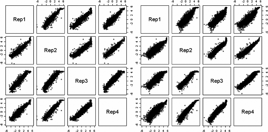
Comparison of gene expression estimates across the four technical replicates for time point 4 of line AB. On the left, the estimates are the ‘best’ scan values. On the right, the estimates are the values from the hierarchical model with three scans. The replicates generally agree with each other except for replicate 1 estimated with one scan. The estimates for replicate 1 using the hierarchical model are more in agreement with the other technical replicates.

Figure 5 shows two genes that have smaller variance among the 12 estimated expression values at each of the five time points when the hierarchical model with three scans is used to estimate the expression values than when one scan is used. A quarter of the genes have a reduction in variance at all five time points; 82% have a reduction in variance at three or more time points. Note that these are normalized values and the combination of scans and normalization were carried out on each slide. There was no shrinkage due to the model for combining scans because it is applied separately for each slide/dye combination. Therefore, this reduction in variance is a side-effect of more accurate estimation within each slide.

Figure 5.

Errorbar plots for two example genes from the 12 normalized replicate expression estimates for each time point. The red lines are estimates from one scan and the black lines use the hierarchical model for three scans. The first gene was censored below on three slides out of 60; the second gene was not censored. Average estimated expression across the 12 replicates does not change substantially except for censored genes. The errorbars from one scan are all larger than the errorbars from the hierarchical model with three scans for these two genes and 25% of the genes in the experiment.

The experimental design used both biological replication among lines and technical replication. Most of the genes have a reduction in variance between the four technical replicates taken for each of the 15 combinations of line and time point; 77% have a reduction in variance of technical replicates at eight or more line and time point combinations. Additionally, the line effects (AB, CD, and EF) were confounded by an order effect because all of the microarrays for each line were prepared and measured at the same time. Samples from line AB were run first, and the raw data from this line is strikingly different from the other two lines (which are fairly similar). When three scans are used to estimate the gene expression values, the three lines show expression patterns over time that are more consistent across lines/running time order. These better estimates of the gene expression values correct somewhat for the difference in procedure between the lines. Again, the combination of scans was carried out separately on each slide. The increased similarity of the expression estimates for technical replicates is not built into the model; rather, it is a side-effect of the increased accuracy of expression estimates.

5.2 Inferences About Time and Line Effects

Also of interest is how the changes to the precision for gene expression estimates affect later analysis and identification of differentially expressed genes. There are many possible analyses that could be applied at this stage including adjusted t test procedures, hierarchical mixture models, and analysis of variance or analysis of covariance models. Similar changes in the quality of conclusions are expected if our estimation method is applied before any technique for identifying differential expression. A hierarchical Gamma-Gamma mixture model for identifying differential expression, of the type in Kendziorski et al. (2003), was applied to these data after the use of all scans to estimate expression in Love and Carriquiry (2005). Here, we apply the related hierarchical lognormal-Normal mixture models to examine the difference in conclusions with the incorporation of all slide readings (see Appendix A.5 for details).

To identify line and time effects we fit hierarchical Normal-Normal mixture models to normalized estimated log-expression for each of the 12,060 genes. We are interested in identifying those genes for which time points have statistically significant differential expression. We designate genes with greater than 50% posterior probability of differential expression under the model as differentially expressed.

When gene expression is estimated using one scan for each gene, 158 genes are identified as exhibiting significant differential expression over time. When the hierarchical model using three scans per slide/dye combination is used to estimate gene expression, 377 genes are found to have significantly different expression levels at different time points, thus indicating that these genes are active during embryo maturation and germination in the somatic embryogenesis experiment.

Note that the number of genes identified as differentially expressed during somatic embryogenesis approximately doubled when all available measurements on each spot were used for analysis. This result was to be expected given the reduction in bias and RMSE in gene expression estimates that was achieved by implementing the procedure we propose. More precise estimates of expression for each slide should lead to less variable estimates of expression for each treatment; this in turn leads to enhanced power to detect significant differential expression. Of the 158 genes that were identified as differentially expressed using only one scan, 75 were also included in the longer list of genes identified when all readings were used. We expect to make Type I errors on individual genes because each gene has at least 50% posterior probability of differential expression whereas the entire list has a smaller probability of being all differentially expressed. Therefore this small amount of overlap is not surprising in the microarray framework. Closer study of the gene lists supports our confidence that the longer list is more useful for continuing study.

A collaborator in Plant Sciences hand-classified the 460 genes identified as differentially expressed using either the standard expression estimation or our proposed method. About 25% were of unknown function and the majority were classified into 27 functional categories. This experiment follows maize embryos through large changes (from small embryos through shoot and root development) and there are consequentially several expected functional patterns of differential expression. The most obvious of these is the activation of photosynthesis during embryo germination (shoot development). Of the 39 genes related to photosynthesis and found to be significantly differentially expressed using either method, 38 are found significantly differentially expressed when combining three scans and only two are identified using one scan. Also, a large number of metabolism genes are expected to be active; there are 18 found with one scan and 50 found with three scans. Finally, an interestingly large number of defense, stress, transcription, translation, and nuclear proteins were identified as differentially expressed in the experiment regardless of which estimation method is used. These unexpectedly active categories of genes are possibly related to somatic embryogenesis (about which little information exists); they are of interest for further investigation. However, these interesting genes are much better identified using the three scans estimates of expression (except for nuclear proteins of which only one additional is found with our method). For example, the five stress genes identified using the standard method are all discovered using the proposed method along with 12 additional stress genes. Whereas five stress genes out of 158 is already an interesting finding, 17 out of 377 is of even greater interest. The 377 genes identified as differentially expressed in the reanalysis of these data more closely match the biological hypotheses regarding expression patterns in this experiment and they find more interesting candidates for further investigation.

6. DISCUSSION

Data collected from a somatic embryogenesis experiment in maize (described in Section 1) were analyzed using standard statistical approaches and results were presented in Che et al. (2004). Even though the collection of genes that were originally identified as differentially expressed was plausible given the nature of the experiment, our collaborators in Plant Sciences had anticipated that a more extensive group of genes with more diverse functions would be included among those suspected to actively participate in the process of embryo formation in maize. In an attempt to extract more information from this experimental dataset, we developed methodology for estimating gene expression values that uses all the measurements routinely made on each spot by study technicians.

The use of multiple scans obtained under the same laser and sensor settings has been proposed as a means to reduce the variability of gene expression estimates (Romualdi et al. 2003). Yet improving homogeneity of spots and accounting for the purely random measurement error should be possible using effective segmentation and background cleaning methods. It has been only recently that some attention has been focused on analytical methods that might permit incorporating multiple slide scans obtained under different measurement conditions into statistical analyses. Several approaches have been proposed in the literature for doing so (Dudley et al. 2002; Lyng et al. 2004; Garcia de la Nava et al. 2004). None of these approaches, however, can incorporate an arbitrary and possibly different number of scans per slide into the analysis. Thus, none can make full use of the information available on each slide.

In this manuscript, we propose a general hierarchical modeling approach that allows incorporation of as many readings as may be available for each slide into the model, even if the number of readings per slide vary across slides. The basic premise is that each reading of a spot contains some information about the true expression of the gene and that if an appropriate scaling factor for each spot can be estimated, then all readings for a spot estimate the same quantity and can be combined. Then it is to be expected that the estimate of gene expression will have smaller variance than it would have if based on a single spot measurement. We show via simulation that gains in expression estimation are accrued in both the bias and the RMSE senses. The somatic embryogenesis experiment provides an argument that the power with which differentially expressed genes can be identified is substantially increased if all information on each slide is used in the analyses.

We make several modeling assumptions in our work. For example, we assume that a single multiplicative factor is associated with expression levels of all spots on a slide. That is, if a specific laser and sensor settings tends to increase expression levels, we assume that the multiplicative factor is uniform across all spots on a slide. Whereas this assumption appeared justified in our embryogenesis experiment, it may not hold in all situations; however modeling each spot within a slide individually makes the problem analytically intractable. Simulation results show that the bias with which we can estimate gene expression is associated with expression levels, indicating that spots in different expression level categories might require different scalings to correct for the effect of the same laser and sensor settings. This is an area for further investigation.

To determine whether the modeling approach we propose results in estimators of gene expression with good statistical properties, we ran a simulation study and assessed bias and root mean squared error of the estimators over repeated sampling. The simulation experiment is described in some detail in Section 4. Using simulated gene expression data, we applied several of the approaches (including the approach proposed here) to estimate gene expression for 10,000 genes and compared the various methods on the basis of bias, RMSE, and the dynamic range of the estimates obtained. The hierarchical modeling approach we propose had smaller bias and smaller RMSE than all other stimators and recovered much of the true range, suggesting that assuming linear scaling and basing estimation on as many readings for each spot as are available is a reasonable idea. Genes with very high and with very low true expression levels were subject to larger biases. This is to be expected because these are the genes that are likely to have censored expression measurements under high or low laser and sensor settings; changes in instrument settings cause not only a shift but also a censoring of the expression measurements in those genes.

While promising, conclusions drawn from the simulation experiment may be overly optimistic. Because the model used to generate the data is similar to that used for analyzing the data, biases and uncertainties in the estimates that may result from actually fitting the wrong model cannot be assessed. Thus, data obtained through simulation, while often quite informative, must be cautiously interpreted. We addressed this issue somewhat by fitting alternative specifications of the model to data generated from alternative models. The results uniformly pointed to improved expression estimates using our method.

We implemented the proposed hierarchical modeling approach on the microarray data from a maize somatic embryogenesis experiment carried out by scientists in the Plant Sciences Institute at Iowa State University (Che et al. 2004). Whereas we present only a subset of the results here, this serves to highlight some of the improvements that appear to be associated with the use of the three scans available for each slide. Though not included here, we have compared expression estimates with our method for this data to those obtained from fitting the hierarchical model using only one reading per slide (to share information across genes); we note that the posterior variance of expression estimates is lower when based on three readings, as would be expected. We also notice that expression levels are not as shrunken toward the mean expression (2,594).

Inferences about the set of genes involved in somatic embryogenesis in maize change drastically when statistical analyses are based on one or on three readings of each slide. This is because of the smaller bias and RMSE in gene expression estimates from our method, as shown in the simulation studies. Here we have indicated that the power of lognormal-Normal mixture models (as in Kendziorski et al. (2003)) to find differential expression increases as the bias and RMSE in gene expression estimates decreases (which results in more precise time and line pool effect estimates). It is expected that a similar increase in the power to identify differentially expressed genes would be observed if analysis of variance, adjusted t-tests, or another differential expression detection method were compared on data using the standard (one scan) expression values and our proposed estimates for gene expression. As Skibbe, Nettleton, and Schnable (2006) pointed out, conclusions drawn about differential expression can be dependent on the slide scan used. Here we see that stronger conclusions about differential expression are possible using all available scans than using only one.

Of more practical importance than simply identifying more differentially expressed genes with the proposed method, are the conclusions that the new list more closely matches the biological hypotheses regarding expression patterns during embryo maturation and germination and finds more interesting candidates for further investigation with regard to somatic embryogenesis. An interestingly large number of defense, stress, transcription, translation, and nuclear proteins were identified as differentially expressed in the experiment regardless of which estimation method is used. These unexpectedly active categories of genes are possibly related to somatic embryogenesis; they are of interest for further investigation. However, these interesting genes are much better identified using the hierarchical model with three scans to estimate expression.

APPENDIX

A.1 Identifiability of the First Likelihood

Consider the first likelihood from Section 3. We have S_ij independently distributed Gamma(a, ψ_iχ_j) for i = 1, …, n and j = 1, …, m + 1. Let L(θ) be the likelihood function, θ₁ = (a, ψ₁, …, ψ_n, χ₁, …, χ_m+1), and θ₂ = (a, ψ₁/2, …, ψ_n/2, 2χ₁, …, 2χ_m+1).

$$\begin{array}{cc}L({\theta }_1)\hfill & ={\displaystyle \prod _{i=1}^n{\displaystyle \prod _{j=1}^{m+1}\frac{{({\psi }_i{\chi }_j)}^a}{\mathrm{\Gamma }(a)}}{S}_{ij}^{a-1}{e}^{-{\psi }_i{\chi }_j{S}_{ij}}}\hfill \\ \hfill & ={\displaystyle \prod _{i=1}^n{\displaystyle \prod _{j=1}^{m+1}\frac{{(({\psi }_i/2)(2{\chi }_j))}^a}{\mathrm{\Gamma }(a)}}{S}_{ij}^{a-1}{e}^{-({\psi }_i/2)(2{\chi }_j)S_{ij}}=L({\theta }_2).}\hfill \end{array}$$

Therefore, this likelihood is not identifiable.

A.2 Marginal Likelihood of (a, a₀, ν)

Consider the joint probability distribution p(S, θ, δ|a, a₀, ν). The marginal likelihood function p(S|a, a₀, ν) is obtained by integrating the joint probability distribution with respect to δ and θ as follows:

$$\begin{array}{cc}p(\mathit{S}|a,a_0,\nu )\hfill & \hfill \\ \hfill & ={\displaystyle \int {\displaystyle \int p(\mathit{S},\mathit{\theta },\mathit{\delta }|a,a_0,\nu )d\mathit{\delta }d\mathit{\theta }}}\hfill \\ \hfill & \propto {\displaystyle \int {\displaystyle \int \mathrm{\Gamma }{(a)}^{-n(m+1)}{\displaystyle \prod _{i=1}^n{\theta }_i^{a(m+1)+a_0-1}}{\displaystyle \prod _{j=1}^m{\delta }_j^{na+{\alpha }_1-1}}}}\hfill \\ \hfill & \hfill {\displaystyle \prod _{i=1}^n{\displaystyle \prod _{j=1}^{m+1}{S}_{ij}^{a-1}}}\\ \hfill & e^{-{\displaystyle {\sum }_{i=1}^n{\theta }_i}{\displaystyle {\sum }_{j=1}^{m+1}{\delta }_j{S}_{ij}-\nu {\displaystyle {\sum }_{i=1}^n{\theta }_i-{\alpha }_2}{\displaystyle {\sum }_{j=1}^{m+1}{\delta }_j}}}d\mathit{\delta }d\mathit{\theta }\hfill \\ \hfill & =\mathrm{\Gamma }{(a)}^{-n(m+1)}{\displaystyle \prod _{i=1}^n{\displaystyle \prod _{j=1}^{m+1}{S}_{ij}^{a-1}}}\hfill \\ \hfill & {\displaystyle \int {\displaystyle \prod _{i=1}^n{\theta }_i^{a(m+1)+a_0-1}}{e}^{-\nu {\displaystyle {\sum }_{i=1}^n{\theta }_i}}}\hfill \\ \hfill & {\displaystyle \int {\displaystyle \prod _{j=1}^m{\delta }_j^{na+{\alpha }_1-1}}{e}^{-{\displaystyle {\sum }_{j=1}^{m+1}{\delta }_j}({\displaystyle {\sum }_{i=1}^n{\theta }_i{S}_{ij}-{\alpha }_2})}d\mathit{\delta }d\mathit{\theta }}\hfill \\ \hfill & =\mathrm{\Gamma }{(a)}^{-n(m+1)}{\displaystyle \prod _{i=1}^n{\displaystyle \prod _{j=1}^{m+1}{S}_{ij}^{a-1}}}\hfill \\ \hfill & {\displaystyle \int {\displaystyle \prod _{i=1}^n{\theta }_i^{a(m+1)+a_0-1}}{e}^{-\nu {\displaystyle {\sum }_{i=1}^n{\theta }_i}}}\hfill \\ \hfill & \mathrm{\Gamma }{(na+{\alpha }_1)}^m{\displaystyle \prod _{j=1}^m({{\displaystyle \sum _{i=1}^n{\theta }_i{S}_{ij}-{\alpha }_2})}^{-(na-{\alpha }_1)}d\mathit{\theta }}\hfill \\ \hfill & =\mathrm{\Gamma }{(a)}^{-n(m+1)}\mathrm{\Gamma }{(na+{\alpha }_1)}^m{\displaystyle \prod _{i=1}^n{\displaystyle \prod _{j=1}^{m+1}{S}_{ij}^{a-1}}}\hfill \\ \hfill & {\displaystyle \int {\displaystyle \prod _{i=1}^n{\theta }_i^{a(m+1)+a_0-1}}{e}^{-\nu {\displaystyle {\sum }_{i=1}^n{\theta }_i}}}\hfill \\ \hfill & {\displaystyle \prod _{j=1}^m({{\displaystyle \sum _{i=1}^n{\theta }_i{S}_{ij}-{\alpha }_2})}^{-(na-{\alpha }_1)}d\mathit{\theta }}.\hfill \end{array}$$

A.3 Marginal Likelihood of (a, a₀, ν) Conditional Only on Largest Reading

The marginal likelihood function p(S_•(m+1)|a, a₀, ν) is obtained by integrating the marginal probability distribution with respect to δ and θ as follows:

$$\begin{array}{cc}p({\mathit{S}}_{•(m+1)}|a,a_0,\nu )\hfill & \hfill \\ \hfill & ={\displaystyle \int {\displaystyle \int p({\mathit{S}}_{•(m+1)},\mathit{\theta },\mathit{\delta }|a,a_0,\nu )d\mathit{\delta }d\mathit{\theta }}}\hfill \\ \hfill & \propto {\displaystyle \int {\displaystyle \int p({\mathit{S}}_{•(m+1)}|a,a_0,\nu ,\mathit{\theta })p(\mathit{\theta }|a_0,\nu )p(\mathit{\delta })d\mathit{\delta }d\mathit{\theta }}}\hfill \\ \hfill & ={\displaystyle \int p({\mathit{S}}_{•(m+1)}|a,a_0,\nu ,\mathit{\theta })p(\mathit{\theta }|a_0,\nu )d\mathit{\theta }}\hfill \\ \hfill & ={\displaystyle \int \mathrm{\Gamma }{(a)}^{-n}{\displaystyle \prod _{i=1}^n{\theta }_i^a}{S}_{i(m+1)}^{a-1}\exp (-{\theta }_i{S}_{i(m+1)})}\hfill \\ \hfill & \mathrm{\Gamma }{(a_0)}^{-n}{\nu }^{n{a}_0}{\displaystyle \prod _{i=1}^n{\theta }_i^{a_0-1}\text{exp}(-\nu {\theta }_i)d\mathit{\theta }}\hfill \\ \hfill & ={\mathrm{\Gamma }(a)\mathrm{\Gamma }(a_0))}^{-n}{\displaystyle \prod _{i=1}^n{S}_{i(m+1)}^{a-1}{\nu }^{n{a}_0}}\hfill \\ \hfill & {\displaystyle \int {\displaystyle \prod _{i=1}^n{\theta }_i^{a+a_0-1}}\text{exp}(-{\displaystyle \sum _{i=1}^n{\theta }_i(S_{i(m+1)}+\nu }))d\mathit{\theta }}\hfill \\ \hfill & =({\frac{{\nu }^{a_0}\mathrm{\Gamma }(a+a_0)}{\mathrm{\Gamma }(a)\mathrm{\Gamma }(a_0)})}^n{\displaystyle \prod _{i=1}^n(\frac{S_{i(m+1)}^{a-1}}{{(S_{i(m+1)}+\nu )}^{a+a_0}}).}\hfill \end{array}$$

A.4 Experimental Design

To compare design strategies, we use the mixed effects model as in Kerr and Churchill (2001). Here, we consider only the observations for one particular gene. The total number of time points, biological lines, and slides were fixed by the experimental conditions at 5, 6, and 30, respectively. We assume that each gene expression number, Y_ijkl, is a random variable resulting from the sum of several fixed and random effects:

$$Y_{ijkl}=\mu +R_i+{\tau }_j+S_{k(i)}+{\delta }_l+{(RT)}_{ij}+e_{ijkl}$$

where

• µ is the grand mean for expression,

• R_i denotes the effect of the ith biological sample and is random, i = 1, …, r where r is the number of biological replications used, and $R_i\sim N\left(0,{\sigma }_R^2\right)$,

• τ_j denotes the effect of the jth time point in the experiment and is fixed, j = 1, …, 5.

• S_k(i) denotes the effect of the kth slide in the ith biological sample and is random, k = 1, …, s where s is the number of slides used for each biological sample, and $S_{k(i)}\sim N\left(0,{\sigma }_S^2\right)$,

• δ_l denotes the effect of the lth dye color and is fixed, l = R, G.

• (RT)_ij denotes the interaction of the biological samples and the time points (to allow for different biological samples to react differently at the same time points) and is random and ${(RT)}_{ij}\sim N\left(0,{\sigma }_{RT}^2\right)$,

• ε_ijkl denotes the random error from the biological replication ${\epsilon }_{ijkl}\sim N\left(0,{\sigma }_e^2\right)$.

We are interested in estimating the difference in gene expression at different time points for a particular gene, τ_m – τ_n where m ≠ n. This is estimated by the average observed difference between the two time points, Ȳ_•m•• – Ȳ_•n••.

The point estimate of the difference in gene expression between two time points m and n is the same under all designs discussed later. However, the variance of the estimate can be affected by the study design. In its most general form the variance is given by

$$\begin{array}{cc}\text{Var}({\overline{Y}}_{•m••}-{\overline{Y}}_{•n••})\hfill & =\text{Var}{\overline{((RT)}}_{•m}-{\overline{(RT)}}_{•n})+\text{Var}({\overline{S}}_{••}(m)\hfill \\ \hfill & -{\overline{S}}_{••}(n))+\text{Var}({\overline{e}}_{•m••}-{\overline{e}}_{•n••}).\hfill \end{array}$$

• Loop Design: A loop design, pairing each sample with a different time point instead of a reference sample, was used within the analysis of each line, see Figure 6. The loop design has been clearly shown to be preferable to a reference design for cDNA microarray experiments (Kerr and Churchill 2001). This means that the variance of the estimate for differential expression, Var(Ȳ_•m•• – Ȳ_•m••), is smaller when using the loop design than the reference design.

• Pooling Samples: The experiment was conducted using six biological samples. Two approaches are of interest: analyze all six lines independently, or pool pairs of lines into three unique biological samples (as done, for example, in Kendziorski et al. 2003 where mRNA from four rats were pooled). We discuss the advantages and disadvantages of each approach in the context of the variance of estimated effects of interest. In both cases, a loop design is assumed.

• Let m and n be any two different time points. For the unpooled design we have

  $$\begin{array}{cc}\hfill & \text{Var}({\overline{Y}}_{•m••}-{\overline{Y}}_{•n••})\hfill \\ \hfill & =\text{Var}{\overline{((RT)}}_{•m}-{\overline{(RT)}}_{•n}+\text{Var}({\overline{S}}_{••}(m)-{\overline{S}}_{••}(n))\hfill \\ \hfill & \hfill +\text{Var}({\overline{e}}_{•m••}-{\overline{e}}_{•n••})\\ \hfill & =\text{var}(\frac{1}{12}(2{\displaystyle \sum _{i=1}^6{(RT)}_{im}-2{\displaystyle \sum _{i=1}^6{(RT)}_{in}}}))+\frac{3{\sigma }_S^2}{24}+\frac{2{\sigma }_e^2}{12}\hfill \\ \hfill & =\text{Var}{\overline{((RT)}}_{•m}-{\overline{(RT)}}_{•n})+\frac{3{\sigma }_S^2}{24}+\frac{2{\sigma }_e^2}{12}\hfill \\ \hfill & =\frac{2{\sigma }_{RT}^2}{6}+\frac{3{\sigma }_S^2}{24}+\frac{2{\sigma }_e^2}{12}.\hfill \end{array}$$ (A.1)
• Correspondingly for the pooled design we have

  $$\begin{array}{cc}\hfill & \text{Var}({\overline{Y}}_{•m••}-{\overline{Y}}_{•n••})\hfill \\ \hfill & =\text{Var}(\frac{1}{12}(4{\displaystyle \sum _{i=1}^3\frac{{(RT)}_{(2i-1)m}+{(RT)}_{(2i)m}}{2}}\hfill \\ \hfill & \hfill -4{\displaystyle \sum _{i=1}^3\frac{{(RT)}_{(2i-1)m}+{(RT)}_{(2i)m}}{2}}))\hfill \\ \hfill & +\frac{3{\sigma }_S^2}{24}+\frac{2{\sigma }_e^2}{12}\hfill \\ \hfill & =\text{Var}(\frac{1}{12}(2{\displaystyle \sum _{i=1}^6{(RT)}_{im}}-2{\displaystyle \sum _{i=1}^6{(RT)}_{in}}))+\frac{3{\sigma }_S^2}{24}+\frac{2{\sigma }_e^2}{12}\hfill \\ \hfill & =\text{Var}({\overline{(RT)}}_{•m}-{\overline{(RT)}}_{•n})+\frac{3{\sigma }_S^2}{24}+\frac{2{\sigma }_e^2}{12}\hfill \\ \hfill & =\frac{2{\sigma }_{RT}^2}{6}+\frac{3{\sigma }_S^2}{24}+\frac{2{\sigma }_e^2}{12}.\hfill \end{array}$$ (A.2)

• Table 5 compares the use of pooled and unpooled samples in terms of the variability of measurements and the estimability of several quantities. Because there is no great interest in the distributions of gene expressions (instead we are mostly interested in their means and variances), we make no firm recommendation on this point. The inclination was toward pooling, because of limitations in the amount of biological matter for the earliest time points. It is reasonable to pool pairs into three samples.

Figure 6.

The microarray double loop design with dye swap for the maize embryogenesis experiment.

Table 5.

Comparison of unpooled and pooled experimental designs

Characteristic	Unpooled (6 lines)	3 Pooled lines
Number of slides per line	5	10
Biological variability in each observation	more	less
Estimability of biological variability	greater	lesser
Estimability of the expression distribution	greater	lesser
Variability in effects of interest	equivalent	equivalent

A.5 The Five Stages of Microarray Analysis

Here we detail the standard methods used for each of the five stages of microarray analysis introduced in Section 2.

1. Spot detection and background correction

The software Imagene was used to read the picture files from the scanner. Because the regularity of the spots created by design in the process of printing, we know the approximate address of each spot. This software used a fixed circle method to segment the spots. This means that at each address where a spot was supposed to be, a circle of fixed diameter was positioned so that there was the greatest difference between pixels inside and outside the spot. Then the intensity of each pixel inside the spot was recorded. It has been demonstrated that segmentation has little effect on microarray analysis results and background selection has more of an effect (Yang, Dudoit, Luu, Lin, and Speed 2001).

The background pixels were selected using the concentric-circle-band method. This means that a second and third concentric circle were placed around the circle identified as the spot and pixels within those two circles were designated as background.

At this point, for each spot on each slide there are approximately 125 spot pixel and 130 background pixel intensity measurements. The mean signal pixel intensity is used as the observed intensity for each spot. The median of the (local) background pixel intensity measurements is used as the estimate of the background effect. Because we assume that the intensity measured in the signal is composed of background and true signal intensity, background values are subtracted from observed values to obtain background-corrected values to be used in further analysis.

Note that because background estimates are local and done separately for each scan, the scanner settings will affect the background estimates in the same manner as the spot intensities. For a particular spot, let E and B be the expression and background values and O_j for j = 1, …, J be the observed measurements on the jth scan. Then, O_j = δ_j(E + B) for j = 1, 2, 3 for each of the three scans. So, we use δ_jE = O_j – δ_jB as the background corrected estimate. Because the background estimates are generated for each scan, whatever scaling (δ_j) is included in them is included without needing to be estimated during background removal.

2. Generating one intensity estimate per slide channel from multiple scans

Two methods are compared: the naive method of choosing one ‘best’ scan and the method of combining all scans detailed in the article. The naive method primarily seeks to choose a scan that reduces censoring at the bottom of the possible signal values (0) and at the top of the possible signal values (65,535). To implement the naive method, the following algorithm was used on uncorrected average signal intensities as an approximation to the commonly used methods:

1. The maximums of average spot intensities on each scan were found.

2. If no scan had a maximum intensity of 65,535,

   • the scan with the highest median value was chosen.

3. Otherwise, if any scans had a maximum intensity less than 65,535,

   • among those, the scan with the highest median value was chosen.

4. Otherwise, if all scans had a maximum intensity of 65,535,

   • the scan with the lowest median value was chosen.

3. Normalization across slides to make them comparable

Normalization can be broken down into two classes, within slide normalization and between slide normalization. In most cases, after suitable within slide normalization has occurred, between slide normalization is no longer necessary. After suitable normalization, there should be no slide effect or dye effect, but possibly a gene by dye interaction.

We assume that there is a systematic bias in the gene expression measurements between the two dyes. For gene j, which is not differentially expressed, we do not expect R_j = G_j on average. Instead, we expect R_j = k_jG_j for some k_j.

The normalization used here is print tip group-intensity dependent normalization (Yang et al. 2002). Each print tip has certain individual characteristics that can cause spots printed by the same print tip to be correlated. Also, spots in the same print tip group (MetaRow and MetaColumn combination) appear in spatially close groups within the slide. Thus print tip groups account for bias due to print tips and act as surrogates for spatial effects on the slide.

Print tip group-intensity dependent normalization assumes that the normalizing constant is a distinct function of intensity for each print tip group, k_j = f_i(R_j*G_j) where i indexes print tip group membership. Therefore, R_j = f_i(R_j*G_j) × G_j for all genes j in print tip group i that are not differentially expressed. When we believe that only a small proportion of genes in our experiment are differentially expressed or there are equal magnitudes of over and under expressed genes, a robust estimator of log f_i(·) is the loess curve of log(R/G) against log(R * G) for print tip group i.

The normalized values used are$R_j^{*}=R_j/\sqrt{f_i(R_j^{*}{G}_j)}\text{and}{G}_j^{*}=G_j\times \sqrt{f_i(R_j^{*}{G}_j)}$

4. Identification of differentially expressed genes

The analysis used to identify differentially expressed genes is a Hierarchical Bayesian lognormal-Normal model as in Kendziorski et al. (2003) with the addition of an effect for line pool. This can be written as the following mixture random effects model for each gene:

$$\text{log}(E_{ijk})={\mu }_i+{\alpha }_j+{\epsilon }_{ijk}$$

where i = 1, …, 5, j = 1, …, 3, and k = 1, …, 4; ${\alpha }_j\sim \mathrm{N}\left(0,{\sigma }_a^2\right)$ is the line effect; ε_ijk ~ N(0, σ²); the vector µ is a mixture of µ₁ × (1, 1, 1, 1, 1) and (µ₁, µ₂, µ₃, µ₄, µ₅) with mixing parameter p; and ${\mu }_i\sim \mathrm{N}({\mu }_0,{\sigma }_m^2)$.

5. Post hoc analysis of differentially expressed genes

No statistical post hoc analysis was done for this article.

REFERENCES

- Armstrong CL, Green CE. Establishment and Maintenance of Friable Embryogenic Maize Callus and the Involvement of L-Proline. Planta. 1985;164:207–214. doi: 10.1007/BF00396083. [DOI] [PubMed] [Google Scholar]
- Carlin BP, Louis T. Bayes and Empirical Bayes Methods for Data Analysis. London: Chapman & Hall; 2000. [Google Scholar]
- Che P, Love TM, Frame BR, Wang K, Carriquiry AL, Howell SH. Gene Expression Program During Maturation and Germination of Somatic Embryos in Maize Cultures. Plant Molecular Biology. 2004;62:1–14. doi: 10.1007/s11103-006-9013-2. [DOI] [PubMed] [Google Scholar]
- Dudley AM, Aach J, Steffen MA, Church GM. Measuring Absolute Expression with Microarrays with a Calibrated Reference Sample and an Extended Signal Intensity Range. Proceedings of the National Academy of Sciences of the United States of America. 2002;99:7554–7559. doi: 10.1073/pnas.112683499. [DOI] [PMC free article] [PubMed] [Google Scholar]
- Garcia de la Nava J, van Hijum S, Trelles O. Saturation and Quantization Reduction in Microarray Experiments using Two Scans at Different Sensitivities. Statistical Applications in Genetics and Molecular Biology. 2004;3 doi: 10.2202/1544-6115.1057. article 11. [DOI] [PubMed] [Google Scholar]
- Green CE, Phillips RL. Plant Regeneration From Tissue Cultures of Maize. Crop Science. 1975;15:417–420. [Google Scholar]
- Kendziorski CM, Newton MA, Lan H, Gould MN. On Parametric Empirical Bayes Methods for Comparing Multiple Groups Using Replicated Gene Expression Profiles. Statistics in Medicine. 2003;22:3899–3914. doi: 10.1002/sim.1548. [DOI] [PubMed] [Google Scholar]
- Kerr MK, Churchill GA. Experimental Design for Gene Expression Microarrays. Biostatistics (Oxford, England) 2001;2:183–201. doi: 10.1093/biostatistics/2.2.183. [DOI] [PubMed] [Google Scholar]
- Love TM. PhD Dissertation. Iowa State University; 2005. Exploring Statistical Methods for Analysis of Microarray Data. [Google Scholar]
- Love TM, Carriquiry AL. Estimating Gene Expression Profiles Using all Available Information. The Proceedings of the 2005 Kansas State University Conference on Applied Statistics in Agriculture. 2005;17:1–32. [Google Scholar]
- Lunn DJ, Thomas A, Best N, Spiegelhalter D. WinBUGS – a Bayesian Modelling Framework: Concepts, Structure, and Extensibility. Statistics and Computing. 2000;10:325–337. [Google Scholar]
- Lyng H, Badiee A, Svendsrud DH, Hovig E, Myklebost O, Stokke T. Profound Influence of Microarray Scanner Characteristics on Gene Expression Ratios: Analysis and Procedure for Correction. BMC Genomics. 2004;5:10. doi: 10.1186/1471-2164-5-10. [DOI] [PMC free article] [PubMed] [Google Scholar]
- Newton MA, Kendziorski CM, Richmond CS, Blattner FR, Tsui KW. On Differential Variability of Expression Ratios: Improving Statistical Inference about Gene Expression Changes from Microarray Data. Journal of Computational Biology. 2001;8:37–52. doi: 10.1089/106652701300099074. [DOI] [PubMed] [Google Scholar]
- Romualdi C, Trevisan S, Celegato B, Costa G, Lanfranchi G. Improved Detection of Differentially Expressed Genes in Microarray Experiments Through Multiple Scanning and Image Integration. Nucleic Acids Research. 2003;31:e149. doi: 10.1093/nar/gng149. [DOI] [PMC free article] [PubMed] [Google Scholar]
- Skibbe DS, Wang X, Zhao X, Borsuk LA, Nettleton D, Schnable PS. Scanning Microarrays at Multiple Intensities Enhances Discovery of Differentially Expressed Genes. Bioinformatics (Oxford, England) 2006;22:1863–1870. doi: 10.1093/bioinformatics/btl270. [DOI] [PubMed] [Google Scholar]
- Swanson-Wagner RA, Jia Y, DeCook R, Borsuk LA, Nettleton D, Schnable PS. All Possible Modes of Gene Action Are Observed in a Global Comparison of Gene Expression in a Maize F1 Hybrid and its Inbred Parents. Proceedings of the National Academy of Sciences of the United States of America. 2006;103:6805–6810. doi: 10.1073/pnas.0510430103. [DOI] [PMC free article] [PubMed] [Google Scholar]
- Tadesse MG, Ibrahim JG, Mutter GL. Identification of Differentially Expressed Genes in High-Density Oligonucleotide Arrays Accounting for the Quantification Limits of the Technology. Biometrics. 2003;59:542–554. doi: 10.1111/1541-0420.00064. [DOI] [PubMed] [Google Scholar]
- Wit E, McClure J. Statistical Adjustment of Signal Censoring in Gene Expression Experiments. Bioinformatics (Oxford, England) 2003;19:1055–1060. doi: 10.1093/bioinformatics/btg003. [DOI] [PubMed] [Google Scholar]
- Yang YH, Dudoit S, Luu P, Lin DM, Peng V, Ngai J, Speed T. Normalization for cDNA Microarray Data: A Robust Composite Method Addressing Single and Multiple Slide Systematic Variation. Nucleic Acids Research. 2002:30. doi: 10.1093/nar/30.4.e15. [DOI] [PMC free article] [PubMed] [Google Scholar]
- Yang YH, Dudoit S, Luu P, Lin DM, Speed T. Normalization for cDNA Microarray Data. Proceedings of SPIE. 2001;4266:19. [Google Scholar]