A black-box re-weighting analysis can correct flawed simulation data

Abstract

There is a great need for improved statistical sampling in a range of physical, chemical, and biological systems. Even simulations based on correct algorithms suffer from statistical error, which can be substantial or even dominant when slow processes are involved. Further, in key biomolecular applications, such as the determination of protein structures from NMR data, non-Boltzmann-distributed ensembles are generated. We therefore have developed the “black-box” strategy for reweighting a set of configurations generated by arbitrary means to produce an ensemble distributed according to any target distribution. In contrast to previous algorithmic efforts, the black-box approach exploits the configuration-space density observed in a simulation, rather than assuming a desired distribution has been generated. Successful implementations of the strategy, which reduce both statistical error and bias, are developed for a one-dimensional system, and a 50-atom peptide, for which the correct 250-to-1 population ratio is recovered from a heavily biased ensemble.

Ensemble averages over configurations are fundamental to the analysis of finite-temperature systems of physical, chemical, and biological interest, as well as to any statistically defined system. Yet it is well appreciated that estimates of such averages based on computer simulations can suffer from both systematic and statistical error (1,2). We therefore ask: Given a set of previously generated configurations of uncertain quality, what is the best way to estimate ensemble averages? Our proposed answer, the “black-box reweighting” (BBRW) strategy described below, appears promising in its ability to overcome both types of error in some systems.

Statistical error is a ubiquitous problem of underappreciated practical importance. Every algorithm known to the authors, including sophisticated methods (3–5), relies on repeated visits to a state (a subset of configuration space) to generate statistical reliability or precision in the population estimate for that state. If we define the simulation-and-system-specific correlation time t_corr as the time required to visit all important states at least once, then statistical precision requires a long total simulation time, t_sim ≫ t_corr. Standard square-root-of-duration arguments (1,2) suggest that a simulation retains a fractional imprecision of $\sqrt{t_{\text{corr}}/t_{\text{sim}}}$ (on a unit scale). Below, we show that BBRW dramatically cuts statistical error, avoiding the slow square-root behavior.

Systematic bias is typical in some systems of great practical importance—such as full-sized proteins—where, to date, it is not clear that any atomically detailed simulation has come close to reaching t_corr. Indeed, surprisingly lengthy simulations are required to obtain statistical ensembles for small peptides (6). Nevertheless, biased non-Boltzmann distributed sets of atomically detailed protein structures are regularly generated, e.g., for NMR structure determination (7) and in the study of protein folding (8). These sets can be useful for docking (9), which is employed in drug design. The proposed BBRW strategy, in principle, can convert such sets into statistically distributed ensembles.

Background and Theory

The fundamental basis of our reweighting approach is the recognition that a simulation's output (the configurations generated) contains valuable information that is not conventionally used to estimate ensemble averages. This information is the observed configuration-space density. It is critical to note that the observed density never matches the targeted distribution (e.g., proportional to a Boltzmann factor) because of (i) the omnipresent statistical error and also, possibly, (ii) errors in the algorithm or software. Our approach can treat both statistical and systematic error because it is blind to the source of error.

Theory.

Standard reweighting theory assumes that configurations in a simulated ensemble are already distributed according to a known distribution, typically proportional to a Boltzmann factor (10–14). The novelty of our reweighting method is that we treat configurations as if they were generated by an unknown process, a “black box.” Thus, any ensemble can be treated because the results of the reweighting do not depend on the specific process that was used to generate the ensemble.

Our goal is to estimate ensemble averages and relative weights for configurations x⃗_j—denoted by j—in the target distribution P(j), regardless of how the configurations were generated. Although our approach will be general, we will assume for concreteness that the target ensemble is a classical system with potential energy U(x⃗). In this case, the targeted probability density is P(j) = Z⁻¹e^{−U(x⃗_j)/k_BT}, where Z = ∫dx⃗e^{−U(x⃗)/k_BT} is the configurational partition function at temperature T. Because Z is typically not known, it will prove useful to define the unnormalized distribution

The overall partition function Z will not affect our quest to assign relative configurational weights.

The sample to be analyzed consists of a set of N configurations {x⃗₁, x⃗₂, …,  x⃗_N} generated by an arbitrary simulation protocol. This set of configurations is distributed according to the observed probability density P^obs(j), by definition. In general, the observed and targeted distributions will differ, P^obs(j) ≠ P(j), because of statistical and/or systematic error as explained earlier. It will again prove useful to consider an unnormalized density denoted by p^obs(j) ∝ P^obs(j).

With the targeted and observed distributions defined, the straightforward logic of standard reweighting (11) may be applied. In an ideal sample, an infinitesimal configuration-space volume dx⃗ about j would contain a quantity of configurations- proportional to the targeted distribution p(j)dx⃗. However, in actuality, p^obs(j)dx⃗ is obtained. The erroneous sampling can be corrected to cancel the error, by applying a relative weight

to each configuration. For the physical systems considered here, the target distribution is given exactly by the standard Boltzmann factor of Eq. 1. Therefore, we assume p is “known” in the sense that it can be evaluated for an arbitrary configuration. Then, because Eq. 2 is exact, the key to practical application of this equation is accurate estimation of p^obs.

Note that the relative weights of Eq. 2 will only be applied to the N configurations already generated—and, therefore, do not report on regions of configuration space not sampled.

Ensemble averages of any function f, in our approach, are given by a weighted sum over sampled configurations x⃗_j:

The average Eq. 3 differs from what we term a “canonical average” of the same configurations, where one assumes p^obs(j) ∝ p(j); then w^bb(j) is a constant, and averages reduce to the usual unweighted estimate ${\langle f\rangle }_{\text{can}}={\displaystyle {\sum }_{j=1}^{N}f(j)/N(2)}$. Note that the proportionality constants for p(j) and p^obs(j) cancel in 3 and thus do not affect the average.

To see why it is better to reweight samples when p^obs can be estimated well, consider the extreme case of a discrete system with six equi-probable states s (e.g., a cubic die). Of course, all ensemble properties can be calculated by hand, but what if statistical sampling were relied upon? Assume N = 30 samples were generated (either by a biased or unbiased procedure), yielding the frequencies (8,4,2,4,7,5), proportional to p^obs(s) for s = (1,…,6), respectively. Clearly, the canonical assumption p^obs ∝ p will lead to substantial errors in ensemble averages. However, the frequencies of observation will exactly cancel p^obs when the relative weights w^bb are used in 3—summing over all 30 “configurations”— to yield exact ensemble averages. The extension of this simple idea to continuum systems is the subject of this report.

Several additional points should be made regarding the strategy embodied in 2 and 3: (i) It is an analysis scheme, treating the same set of configurations as might be analyzed canonically; the approach is not capable of predicting populations for regions of configuration space that are not in the observed ensemble. (ii) The observed relative probabilities {p^obs(j)} will always differ from those intended (e.g., canonical Boltzmann factors) due to statistical error—and perhaps significantly. (iii) The relative weights Eq. 2 are valid regardless of the specific process used to generate configurations. (iv) The approach is particularly suited to estimating conformational free energy differences, as described below. (v) As in the single histogram approach (10), the BBRW method retains the ability to reweight configurations into an arbitrary target ensemble p. (vi) The principal practical challenge in implementing our strategy is the estimation of p^obs.

Free Energy Differences.

To provide a proof of principle for our reweighting approach, we will determine free energy differences (ΔF), between states for various test systems (15–21).

A well established canonical technique for determining ΔF is to use ordinary simulation methods (e.g., molecular dynamics) to generate an ensemble that is distributed according to the desired distribution p. Then, the free energy difference is defined as

where $Z_s={\displaystyle {\int }_{\vec{x}\in s}d\vec{x}{e}^{-U(\vec{x})/k_{B}T}}$ is the configurational partition function for state s with coordinates given by x⃗, and N_s is the number of configurations observed in state s.

For our reweighting approach, we do not assume that configurations are distributed according to p. Instead, each configuration must first be assigned a relative weight using Eq. 2; then ΔF is estimated based on summing these weights in the respective states:

where ${\displaystyle {\sum }_{j\in s}}$ represents a sum over all relative weights w^bb(j) in the state s.

One-Dimensional Thought Experiment.

The central idea behind our reweighting approach is that one can utilize the observed configuration-space density to reweight an arbitrary set of configurations into any desired ensemble. Because this idea is so fundamental to the present discussion, and apparently novel, it is useful to illustrate the idea by using a one-dimensional potential.

Consider the equal-energy double-square-well system depicted in Fig. 1, for which we would like to estimate the relative populations of the two states. Assume that the barrier is so high that it cannot be crossed in a conventional simulation of affordable length, but that we can run independent simulations in each state (a common situation for biomolecular systems when multiple structures are known). The states' widths are in the ratio 1:10.

Fig. 1.

One-dimensional potential for a “thought experiment.” The energy is constant and equal in both states, but the right state is 10 times as wide as the left.

After generating, say, equi-sized trajectories in each state, a conventional view would hold that no analysis of the relative populations is possible because the barrier has not been crossed. However, because the right well is 10 times wider than the left, the observed configuration-space density in the right well will be, on average, one-tenth that in the left. Combined with knowledge of the two ensemble sizes, this is sufficient information for calculating the state populations.

More explicitly, one can estimate the observed density by counting configurations in equi-sized histogram bins, leading to p^obs(j) ∝ n_b(j), where n_b(j) is the count in the bin containing configuration j. In this example, p(j) = const for all j because the energy is constant over both states. Now, by using Eq. 2 in Eq. 5, the sum over relative weights leads to exact cancellation of n_b for each bin. Thus, this purely entropic case is correctly handled, ultimately yielding simply the ratio of the numbers of (equi-sized) bins in each state—i.e., the ratio of state widths. Below, we will see that the “easier” energetic effects are also treated correctly in less trivial examples.

The key point is that the observed density p^obs, combined with knowledge of the desired ensemble p, provides sufficient information to deduce the state populations, regardless of the sampling bias. Perhaps equally importantly, we note that the density can be estimated in different ways besides binning, e.g., by using configuration-space distances between nearby configurations.

The reasoning used to correct systematic bias can be applied equally to statistical error. Assume now that we possess a single continuous trajectory that has crossed the barrier in Fig. 1 at least once. The population estimates will be statistically flawed because of finite sampling. Yet, our reweighting analysis will still yield correct results because the approach does not depend on the source of the bias in the data.

Below we will show that such density information is both present and often accessible in high-dimensional systems. We emphasize that the information is always present in principle and does not depend on prior knowledge.

Results and Discussion

How can the observed density be computed in a way that will be useful, even for high-dimensional systems? We will explore two distinct strategies: binning and also the use of configuration-space distances (“nearest-neighbors strategy”). For high-dimensional systems, we will demonstrate that not all coordinates need be considered in the analysis. We emphasize that other strategies for estimating density are possible (22,23).

The test systems chosen for this study are a one-dimensional double-well potential and a 50-atom dileucine peptide [ACE-(leu)₂-NME]. Our reasoning for choosing these systems are as follows: (i) The system sizes are small enough that it is possible to compute an independent ΔF estimate via counting, i.e., using Eq. 4. (ii) Both are nontrivial: The one-dimensional potential has high barrier, and dileucine has large side chains and thus 144 degrees of freedom.

Binning Strategy.

In the simplest use of bins, the observed density is estimated on the basis of simple counting: omitting normalization, p^obs(j) = n_b(j), where n_b(j) is the number of configurations in the bin that includes configuration j. Indeed, we have tried this scheme and it works, but not optimally.

A more effective procedure for weighting individual configurations combines simple counting with the assumption of local equilibration: Within bins, configurations are assumed distributed according to p itself. This assumption could correspond to the case where separate canonical simulations have been performed in different regions of configuration space, or to a canonical simulation that was not equilibrated on long time scales but well sampled locally. The local-equilibration estimate for the observed distribution is

which implies w^bb(j) = p̄_j/n_b(j). The bin-specific normalization is the average relative target probability in the bin, namely, ${\overline{p}}_j={\displaystyle {\sum }_{i\in \text{bin}}p(i)}/n_b(j)$. This normalization serves to keep the total observed probability of a bin proportional to the number of counts, and independent of the local Boltzmann factors. As explained in the Supporting information (SI) Appendix, a consequence of adopting the approximation Eq. 6 is that p̄_j is implicitly assumed proportional to the local partition function for the bin containing configuration j. (Each bin has a different local partition function estimate.) Nevertheless, we emphasize that the use of local partition functions is not intrinsic to the black-box approach, but only to binning methods for estimating p^obs: See, for instance, the nearest-neighbor strategy described below.

One-dimensional double-well potential.

Here we consider the smooth potential of Fig. 2a. The relative target probability is defined by p(x) = e^-U(x)/k_BT, where U(x) is the potential energy sketched for the approximately 6 k_BT barrier height used here. The barrier heights for this potential, as well as basin curvatures and separations, are fully adjustable, by using, $U(x)=-\ln \left[\exp (-0.5{(x-x_a)}^6-{(x-x_a)}^2/2s_a^2)+\exp (-0.003{(x-x_b)}^4)-{(x-x_b)}^2/2s_b^2\right]$, where we have used x_a = 2.0, x_b = 8.0, s_a = 0.5, and s_b = 1.5. We estimated the ratio of partition functions for the two wells (right over left) using data obtained from ordinary canonical simulation, i.e., Metropolis Monte Carlo (MC) (24).

Fig. 2.

Results for a one-dimensional double-well test system. (a) The potential energy plotted as a function of the coordinate. (b) The ratio of partition functions between the left and right wells. All results shown are the average of 10³ independent computations. The canonical estimates (squares) are given by Eq. 4, the black-box estimates (circles) by Eq. 5. An independent estimate, obtained via integration, is shown by the solid horizontal line. (c) The standard deviation from the same data as that for b is plotted showing the rapid decrease in the standard deviation for our method (circles) as compared to canonical (squares). (d) Estimate of the ratio of partition functions using our reweighting approach via Eq. 5, based on a heavily biased ensemble of configurations. Note that canonical estimation using Eq. 4 is not possible.

Fig. 2 shows the differences between reweighting, by using a binning strategy, and canonical estimates of the ratio of partition functions between two wells (right over left) in Fig. 2a. Results shown are the averages in Fig. 2b and standard deviations in Fig. 2c from 10³ independent computations. The canonical estimates (squares) were computed via 4, and the black-box estimates (circles) via Eqs. 5 and 6 with a bin size of 0.005. All data were generated using the same MC trajectories, each initiated from the left basin of the potential in Fig. 2a. Specifically, all MC trajectories were generated by starting the system at x = 2.0. Each trajectory consisted of 10⁶ trial moves generated by adding a uniform random deviate between -1.0 and 1.0 to the current position. An independent estimate, obtained via numerical integration, is shown by the solid horizontal line in Fig. 2b. Note that in Fig. 2b, the apparent accuracy of canonical estimation at short times represents only the average behavior; the statistical uncertainty is so large that any individual estimate would be completely unreliable.

Fig. 2c demonstrates that the error in our reweighting analysis decreases at a rate greater than the typical square-root behavior, as seen for the canonical error. Because the same ensembles were used for both the reweighting and canonical estimates, this improvement may lead one to believe we are getting something for nothing. In fact, there are costs, but in essence, they have already been paid: (i) The reweighting approach requires knowledge of the desired distribution; in our case (and most other cases of interest), this is given by the Boltzmann factor. (ii) The observed density is available information that is not generally used for analysis of simulation data, and it requires only a small additional computational cost.

In Fig. 2d, we show that our reweighting approach can be used to estimate the correct populations between the left and right wells, with an example that simply cannot be treated canonically. We generated a biased ensemble, with configurations that were not distributed according to p (Boltzmann factor for U shown in Fig. 2a). Then Eqs. 5 and 6 were used with a bin size of 0.005 to estimate the ratio of partition functions. The data show the averages (circles) and standard deviations (error bars) for 10³ independent computations. Because our reweighting approach is independent of the method used to generate the ensemble, we are able to obtain the correct ratio, even though the ensemble used in the analysis was heavily biased. For completeness, we note that the biased ensemble configurations were generated by using the same MC protocol as above, but with a square well potential defined as U(x) = 0 between x = 0 and x = 15 and infinite elsewhere.

Dileucine peptide.

In this high-dimensional molecular example, we again apply our approach to a biased ensemble, where canonical estimation would be meaningless. We use the BBRW method to estimate the free energy difference ΔF between conformational states of the 50-atom dileucine peptide based on independent simulations of each state. The two states considered were defined by backbone dihedrals angles: alpha, -140.0 < Φ_1,2 < -80.0 and -120.0 < Ψ_1,2 < -60.0, and beta, -125.0 < Φ_1,2 < -65.0 and 120.0 < Ψ_1,2 < 180.0.

To test the accuracy of the results from our reweighting approach, we also generated an independent estimate of ΔF. An ordinary, unrestrained, 1.0 μs simulation was performed and analyzed via Eq. 4, yielding ΔF_ind ≈ -3.3 ± 0.1 kcal/mol, with statistical error estimated via block averaging (25). The simulation data were generated using TINKER 4.2 with the OPLS-AA forcefield (26). A 1.0-fs timestep was utilized, and the simulation was coupled to a 300.0 K bath by using the Andersen thermostat (27). Solvation was provided by the generalized Born surface area (GBSA) implicit model (28).

To generate a BBRW estimate based on the locally equilibrated scheme of Eq. 6, simulations of dileucine were performed constrained to either the alpha or beta state. We generated 500,000 configurations in each state based on a total of ≈104 ns. Bins used in Eq. 6 were constructed uniformly by using only the four backbone dihedrals—out of 144 degrees of freedom—leading to a four-dimensional histogram. Note that empty bins, which are expected for physical and statistical reasons, simply do not contribute to averages computed via Eq. 3, because only sampled configurations are summed over.

Fig. 3a shows that our reweighting approach can be used to correctly predict the free energy difference between the alpha and beta states of dileucine. The solid horizontal line is the independent estimate ΔF_ind computed via Eq. 4 with an approximate error determined by block averaging (25). The circles are results from our reweighting method using the backbone dihedral angles Φ and Ψ for both residues. These data were computed by using Eqs. 2, 5, and 6, and plotted as a function of the number of bins used per dihedral angle in the histograms. Even though an equal number of alpha and beta configurations were utilized in our analysis, the ratio of ≈250 is recovered. Note that our strategy, as shown here, is an example of an end-point free energy difference method, because no path connecting alpha and beta is needed (e.g., refs. 15–21).

Fig. 3.

Results for dileucine peptide. (a) The free energy difference between the alpha and beta states of dileucine from binning. Results from our reweighting approach using a heavily biased ensemble are shown. Data were generated by using Eqs. 2, 5, and 6, using only the backbone dihedrals Φ and Ψ. The independent estimate is shown by the solid horizontal line with an error bar determined by block averaging (25). (b) Box-counting analysis of dileucine configurations used to determine the range of bin sizes for a.

Fig. 3a also demonstrates a certain robustness in the approach: There is a broad range of bin sizes that can be used generate the correct free energy difference.

Two criteria were used to determine the range of bin sizes used for the reweighting results in Fig. 3a: (i) The range of bin sizes for accurate ΔF estimation apparently corresponds to the power-law regime of a plot for estimating the box counting dimension (29). This plot is shown in Fig. 3b, where the linear regions denote the power-law behavior. (ii) The extreme bin size results are known exactly. If one bin per dihedral angle is chosen, then the estimate will always be poor and ΔF = 0 (for equi-sized ensembles). At the other extreme, if a very large number of bins per dihedral angle is used, then each bin will have a count of 1, and p^obs = 1 for every structure. Because no true density information is obtained near either extreme, we excluded such estimates.

Nearest-Neighbors Strategy.

In addition to the binning implementation above, we now estimate p^obs of Eq. 2 by computing distances between conformations. The motivation behind pursuing such nonbinning approaches is the realization that for biomolecular systems, it may prove difficult to populate the necessary high-dimensional histogram bins. The number of bins will increase exponentially with the number of coordinates, but the density of sampling in configuration space can always be estimated on the basis of “distances” in configuration space.

In general, to implement the nearest-neighbors strategy (30), the distances between all configurations in the ensemble are computed, by using any metric that preserves the Cartesian volumes intrinsic to partition functions. By definition, the dimensionality of the metric can be as large as the number of degrees of freedom needed to describe a conformation. The observed configuration-space (relative) density for structure j is then given by

which implies w^bb = p(j) R_hyp(j)^d/N_dist(j). Here, R_hyp(j) is the radius of the hypersphere centered on structure j enclosing N_dist(j) structures, and d is the dimensionality of the distance metric used. Typically, as we will demonstrate below, d can be chosen to be much smaller than the dimensionality of the system. See SI Appendix for further discussion of the approximations entailed when d is less than the full dimensionality of the system.

We used Eq. 7 to estimate p^obs for a particular structure j using the following implementation: (i) Compute the distance (by using any appropriate metric) between structure j and all other structures in the ensemble. (ii) Choose a value of N_dist. The radius of the hypersphere R_hyp is given by the distance to the N_dist nearest neighbor. For example, if N_dist = 10 is chosen, then R_hyp is given by the distance to the tenth nearest neighbor.

We tested the approach embodied in Eq. 7 by estimating the free energy difference ΔF between the alpha and beta conformations of dileucine, using the same restrained (thus biased) ensemble that was used above. Following the previous success of using only the torsion angles of dileucine, we chose to use a dihedral angle distance between structures j and k defined by

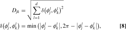where φ^l could be any dihedral angle (e.g., Φ₁, Ψ₂, χ₁), and d is the number of angles used in the computation, i.e., the metric dimension.

Fig. 4 shows that our reweighting approach, using the nearest-neighbors strategy, can be used to predict the free energy difference between the alpha and beta states of dileucine. The solid horizontal line is the independent estimate ΔF_ind computed via Eq. 4 with an approximate error determined by block averaging (25). The circles are results from our reweighting method using the backbone dihedral angles Φ and Ψ from both residues. These data were computed by using Eqs. 2, 5, and 7, with distances given by Eq. 8. The results are plotted as a function of the number of neighbors used in the analysis procedure, N_dist. Even though an equal number of alpha and beta configurations were utilized in our analysis, the ratio of ≈250 is again recovered.

Fig. 4.

The free energy difference (ΔF) between the alpha and beta states of dileucine from a nearest-neighbors strategy. Results from our reweighting approach using a heavily biased ensembles are shown. Data were generated by using Eqs. 2, 5, and 7, with distances computed via Eq. 8. The analysis used only the backbone dihedrals Φ and Ψ. Data are given as a function of the number of distances (neighbors) used in the analysis. The independent estimate is shown by the solid horizontal line with an approximate error determined by block averaging (25).

The accuracy of the nearest-neighbors strategy (or at least the way we implemented the idea) appears to be lower than that of the binning approach; see Fig. 3a. However, the results in Fig. 4 are encouraging, and demonstrate that it is possible to estimate p^obs using a nonbinning procedure.

Note on Efficiency.

It is worthwhile to briefly discuss the efficiency of the reweighting approach using Eq. 5 compared with that of using Eq. 4. There are, in general, two extreme cases to consider: (i) The barrier between the states of interest is very low. This implies that barrier crossing events occur frequently, and thus counting via Eq. 4 will likely be the most efficient approach. (ii) The barrier between the states is too high to cross during ordinary simulation. In this case, counting via Eq. 4 is not possible. Importantly however, the reweighting approach of Eq. 5 can still be utilized because all that is required are independent simulations in each state.

The fairly lengthy simulations required for the BBRW method in the case of dileucine reflects the choice of state definitions: within each state, i.e., alpha or beta, the rotameric (side-chain) timescales are substantially longer than those of the backbone torsions.

Dimensionality.

With dileucine we were able to obtain accurate results for p^obs, and thus ΔF, by using only four degrees of freedom—out of a possible 144. The underlying assumption is that the the degrees of freedom not included in the analysis will provide the same contribution to each relative weight (see SI Appendix for details). Thus, at a minimum, the coordinates used to define the states of interest must be included in the reweighting analysis (here, the backbone dihedrals Φ and Ψ).

A particularly promising strategy for the future is to use principal components analysis, or related methods, to suggest an optimal reduced set of coordinates (15,31,32). These collective coordinates can then be used for binning or to determine configuration-space distances for the nearest-neighbor approach.

Conclusions

The BBRW strategy computes ensemble averages for any target distribution based on estimating the observed configuration-space density actually sampled in a simulation—without employing typical assumptions about sampling quality. In principle, the approach can be used to reweight any ensemble, regardless of the process used to generate the configurations. Our data show that using BBRW can dramatically reduce both systematic and statistical error for some systems.

As a proof of principle, we used the approach to estimate free energy differences (ΔF) for nonoverlapping states of one-dimensional and molecular systems, based on completely independent ensembles generated in each state. Further, when ordinary one-dimensional trajectories exhibiting transitions between states were reanalyzed with BBRW, statistical error was substantially reduced.

Practical application of BBRW hinges on estimation of the observed configuration-space density, p^obs, but the theoretical basis does not. We have obtained reasonable results using two different methods for estimating p^obs, emphasizing that the central idea behind our re-weighting approach is independent of the specific strategy used to estimate p^obs. Strategies beyond those examined in this report are available (22,23) and will be explored in future work.

There are two primary limitations of the overall approach. First, improved density estimation schemes will be needed for higher-dimensional systems. Second, BBRW is an analysis method that reweights configurations in existing ensembles; thus, it cannot predict populations for regions of configuration space not represented in the original data.

Our motivation for the black-box approach stems from the still-outstanding challenge of producing statistical ensembles for full-sized proteins. The black-box approach seems promising in this context because: (i) Non-Boltzmann-distributed sets of diverse structures can be generated by using a variety of methods, including NMR structure prediction software (7), and by the addition of atomic detail to coarse models (8,33). (ii) Local canonical sampling based on ad hoc starting structures is readily possible with existing software. (iii) Our own box-counting studies of proteins (unpublished work) suggest that folded proteins act as systems with dramatically reduced dimensionality; see also refs. 31 and 32. We also hope that BBRW will prove useful in reweighting implicitly solvated biomolecules into explicit solvent ensembles. Finally, the idea could prove of value in the analysis of data from insufficiently converged canonical simulation of any type.

References

- 1.Landau DP, Binder K. A Guide to Monte Carlo Simulations in Statistical Physics. Cambridge, UK: Cambridge Univ Press; 2000. [Google Scholar]
- 2.Frenkel D, Smit B. Understanding Molecular Simulation: From Algorithms to Applications. San Diego: Academic; 1996. [Google Scholar]
- 3.Swendsen RH, Wang J-S. Replica Monte Carlo simulation of spin-glasses. Phys Rev Lett. 1986;57:2607–2609. doi: 10.1103/PhysRevLett.57.2607. [DOI] [PubMed] [Google Scholar]
- 4.Berg BA, Neuhaus T. Multicanonical algorithms for first order phase transitions. Phys Lett B. 1991;267:249–253. doi: 10.1103/PhysRevLett.68.9. [DOI] [PubMed] [Google Scholar]
- 5.Lyman E, Ytreberg FM, Zuckerman DM. Resolution exchange simulation. Phys Rev Lett. 2006;96:028105. doi: 10.1103/PhysRevLett.96.028105. [DOI] [PubMed] [Google Scholar]
- 6.Lyman E, Zuckerman DM. Ensemble-based convergence analysis of biomolecular trajectories. Biophys J. 2006;91:164–172. doi: 10.1529/biophysj.106.082941. [DOI] [PMC free article] [PubMed] [Google Scholar]
- 7.Spronk CAEM, Nabuurs SB, Bonvin AMJJ, Krieger E, Vuister GW, Vriend G. The precision of NMR structure ensembles revisited. J Biomol NMR. 2003;25:225–234. doi: 10.1023/a:1022819716110. [DOI] [PubMed] [Google Scholar]
- 8.De Mori GMS, Micheletti C, Colombo G. All-atom folding simulation of the villin headpiece from strochastically selected coarse-grained structures. J Phys Chem B. 2004;108:12267–12270. [Google Scholar]
- 9.Knegtel RMA, Kuntz ID, Oshiro CM. Molecular docking to ensembels of proteins. J Mol Biol. 1997;266:424–440. doi: 10.1006/jmbi.1996.0776. [DOI] [PubMed] [Google Scholar]
- 10.Ferrenberg AM, Swendsen RH. Optimized Monte Carlo data analysis. Phys Rev Lett. 1989;63:1195–1198. doi: 10.1103/PhysRevLett.63.1195. [DOI] [PubMed] [Google Scholar]
- 11.Liu JS. Monte Carlo Strategies in Scientific Computing. New York: Springer; 2001. [Google Scholar]
- 12.Lee HK, Okabe Y. Reweighting for nonequilibrium Markov processes using sequential importance sampling methods. Phys Rev E. 2005;71:015102. doi: 10.1103/PhysRevE.71.015102. [DOI] [PubMed] [Google Scholar]
- 13.Shehu A, Clementi C, Kavraki LE. Modeling protein conformational ensembles: From missing loops to equilibrium fluctuations. Proteins. 2006;65:164–179. doi: 10.1002/prot.21060. [DOI] [PubMed] [Google Scholar]
- 14.Abreu CRA, Escobedo FA. A general framework for non-Boltzmann Monte Carlo sampling. J Chem Phys. 2006;124:054116. doi: 10.1063/1.2165188. [DOI] [PubMed] [Google Scholar]
- 15.Karplus M, Kushick JN. Method for estimation the configurational entropy of macromolecules. Macromolecules. 1981;14:325–332. [Google Scholar]
- 16.Xiang Z, Soto CS, Honig B. Evaluating conformational free energies: The colony energy and its application to the problem of loop prediction. Proc Natl Acad Sci USA. 2002;99:7432–7437. doi: 10.1073/pnas.102179699. [DOI] [PMC free article] [PubMed] [Google Scholar]
- 17.Chang CE, Gilson MK. Free energy, entropy, and induced fit in host-guest recognition. J Am Chem Soc. 2004;126:13156–13164. doi: 10.1021/ja047115d. [DOI] [PubMed] [Google Scholar]
- 18.White RP, Meirovitch H. A simulation method for calculating the absolute entropy and free energy of fluids: Application to liquid argon and water. Proc Natl Acad Sci USA. 2004;101:9235–9240. doi: 10.1073/pnas.0308197101. [DOI] [PMC free article] [PubMed] [Google Scholar]
- 19.Cheluvaraja S, Meirovitch H. Simulation method for calculating the entropy and free energy of peptides and proteins. Proc Natl Acad Sci USA. 2004;101:9241–9246. doi: 10.1073/pnas.0308201101. [DOI] [PMC free article] [PubMed] [Google Scholar]
- 20.Ytreberg FM, Zuckerman DM. Simple estimation of absolute free energies for biomolecules. J Chem Phys. 2006;124:104015. doi: 10.1063/1.2174008. [DOI] [PubMed] [Google Scholar]
- 21.Ytreberg FM, Zuckerman DM. Peptide conformational equilibria computed via a single-stage shifting protocol. J Phys Chem B. 2005;109:9096–9103. doi: 10.1021/jp0510692. [DOI] [PubMed] [Google Scholar]
- 22.Silverman BW. Density Estimation for Statistics and Data Analysis. London: Chapman and Hall; 1986. [Google Scholar]
- 23.Scott DW. Multivariate Density Estimation: Theory, Practice, and Visualization. New York: Wiley; 1992. [Google Scholar]
- 24.Metropolis N, Rosenbluth AW, Rosenbluth MN, Teller AH, Teller E. Equation of state calculations by fast computing machines. J Chem Phys. 1953;21:1087–1092. [Google Scholar]
- 25.Flyvbjerg H, Petersen HG. Error estimates on averages of correlated data. J Chem Phys. 1989;91:461–466. [Google Scholar]
- 26.Jorgensen WL, Maxwell DS, Tirado-Rives J. Development and testing of the OPLS all-atom force field on conformational energetics and properties of organic liquids. J Am Chem Soc. 1996;117:11225–11236. [Google Scholar]
- 27.Andersen HC. Molecular dynamics simulations at constant pressure and/or temperature. J Chem Phys. 1980;72:2384–2393. [Google Scholar]
- 28.Still WC, Tempczyk A, Hawley RC. A general treatment of solvation for molecular mechanics. J Am Chem Soc. 1990;112:6127–6129. [Google Scholar]
- 29.Strogatz SH. Nonlinear Dynamics and Chaos: With Applications in Physics, Biology, Chemistry, and Engineering. Reading, MA: Addison-Wesley; 1994. [Google Scholar]
- 30.Hnizdo V, Darian E, Fedorowicz A, Demchuk E, Li S, Singh H. Nearest-neighbor nonparametric method for estimating the configurational entropy of complex molecules. J Comput Chem. 2007;28:655–668. doi: 10.1002/jcc.20589. [DOI] [PubMed] [Google Scholar]
- 31.Teodoro ML, Phillips GN, Kavraki LE. Understanding protein flexibility through dimensionality reduction. J Comput Biol. 2003;10:617–634. doi: 10.1089/10665270360688228. [DOI] [PubMed] [Google Scholar]
- 32.Das P, Moll M, Stamati H, Kavraki LE, Clementi C. Low-dimensional, free-energy landscapes of protein-folding reactions by nonlinear dimensionality reduction. Proc Natl Acad Sci USA. 2006;103:9885–9890. doi: 10.1073/pnas.0603553103. [DOI] [PMC free article] [PubMed] [Google Scholar]
- 33.deBakker PIW, DePristo MA, Burke DF, Blundell TL. construction of polypeptide fragments: Accuracy of loop decoy discrimination by an all-atom statistical potential and the AMBER force field with the Generalized Born solvation model. Proteins Struct Funct Genet. 2002;51:21–40. doi: 10.1002/prot.10235. [DOI] [PubMed] [Google Scholar]