A Semilogarithmic Scale for Glucose Provides a Balanced View of Hyperglycemia and Hypoglycemia

Abstract

Objective

It would be desirable to improve the ability of physicians and patients to identify hypoglycemic episodes when viewing displays of glucose by date, time of day, or day of the week.

Research Design and Methods

A logarithmic scale is utilized for display of glucose versus date and time of day using a range of 40 to 400 mg/dl. Several plausible alternatives are considered for transformation of the glucose data.

Result

Use of a semilogarithmic plot triples the percentage of the vertical axis allocated to hypoglycemia (e.g., 40–80 mg/dl) from 10% to 30.1% while compressing the hyperglycemic region. The log scale improves the symmetry of the glucose distribution. Transformations were evaluated corresponding to the Schlichtkrull M₁₀₀ value, the high blood glucose index/low blood glucose index of Kovatchev and associates, an index of glycemic control developed by the present author, and the GRADE score of Hill and coworkers. Results are similar for all four transformations. This approach is applicable both to self-monitoring of blood glucose (SMBG) and continuous glucose monitoring (CGM). Based on preliminary results, it is proposed that the log transform could potentially facilitate analysis of glucose patterns and may facilitate rapid and consistent detection and appreciation of the severity and consistency of hypoglycemic episodes, even in the presence of complex overlapping patterns commonly observed in both SMBG and CGM glucose profiles.

Conclusion

Display of glucose on a logarithmic scale can potentially improve the accuracy of analysis and interpretation of popular methods for graphic display of glucose values. Device manufacturers should consider including options for semilogarithmic display of glucose on SMBG meters, CGM sensors, and software for retrospective analyses of glucose data.

Introduction

Hypoglycemia presents greater acute risks to patients with diabetes than does hyperglycemia, both in terms of acute symptomatology and in terms of cardiac events and mortality.^1–3 However, when glucose data are examined graphically using an arithmetic scale, the maximal negative excursion for hypoglycemia is typically only 40 mg/dl, the difference between a commonly used lower limit for the target range of 80 mg/dl and the lowest measureable value, e.g., 40 mg/dl. In contrast, hyperglycemic excursions might range from 140 to 400 mg/dl or more, i.e., a range of at least 260 mg/dl, which is 6.5-fold larger than the magnitude of the maximal excursion for hypo-glycemia. Because of this asymmetry, it is easy for the physician and patient to overlook hypoglycemic values on graphic displays. When presented with a graph such as that shown in Figure 1A (linear glucose versus date) or Figure 1B (linear glucose versus time of day), one may fail to appreciate the presence or severity of hypo-glycemia, even if those patterns are serious, recurrent, and consistent. Data regarding the frequency of this potential problem in cognition and other errors in interpretation of self-monitoring of blood glucose (SMBG) and continuous glucose monitoring (CGM) data are not available in the literature, although anecdotal evidence suggests that it could have adverse consequences for clinical care.

Figure 1.

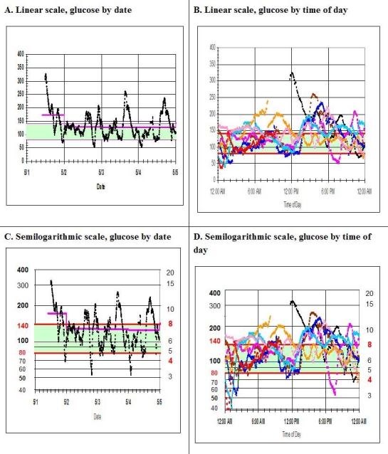
(A) Display of glucose by date for CGM data of one patient for 8 days (linear scale). Vertical axis, glucose (mg/dl); horizontal axis, date. The daily mean glucose is also shown for each day (pink line). (B) Display of glucose profile by time of day for the data of 1A (linear scale). Vertical axis, glucose (mg/dl); horizontal axis, time of day. (C) Glucose by date with glucose displayed on semilogarithmic scale for the same data as 1A. Vertical axis, glucose (mg/dl) on logarithmic scale; horizontal axis, date. (D) Glucose profile by time of day (glucose displayed on logarithmic scale) for the same data as shown in 1B. Vertical axis, glucose (mg/dl) on logarithmic scale; horizontal axis, time of day. The target range of 80–140 mg/dl is shaded light green with red horizontal lines at the upper and lower limits of that range. Values of 50, 100, 200, and 400 mg/dl are emphasized because they are equally spaced on a logarithmic scale. Glucose is shown in units of mg/dl on the left vertical axes and in units of mmol/liter on the right vertical axes of 1C and 1D.

Methods

Several data sets^4–6 have been utilized from CGM and SMBG to examine the effectiveness of a variety of transformations of the scale for glucose in terms of the ability to identify patterns and potential clinical problems involving hypoglycemia, hyperglycemia, or both. A series of transformations were examined, including the common logarithm (log-base-10) and transformations based on the principles underlying the Schlichtkrull M_R index,⁷ the index of glycemic control (IGC),^8,9 the high blood glucose index (HBGI) and low blood glucose index (LBGI) as introduced by Kovatchev and coworkers,^10,11 and the GRADE score as introduced by Hill and associates.¹² These transformations were examined alone or in various combinations. Data have been utilized from studies of CGM, SMBG, and synthetic data sets generated by numerical simulations corresponding to both CGM and SMBG data.

Examined transformations include the following:

1. Logarithmic (use of common logs): G′ = log₁₀(glucose) or log(glucose/R), where R is a reference value, e.g., 100 mg/dl.

2. Linear scale below a specified threshold or cut point and a different linear relationship above that cut point, i.e., different scaling factors for hypoglycemic and hyperglycemic ranges:

   1. If glucose < R, G′ = R + (glucose – R)/c.

   2. If glucose ≥ R, G′ = R + (glucose – R)/d.

      If R = 100 mg/dl, c = 1, and d = 2, this would correspond to a relative expansion of the scale for glucose values below 100 mg/dl by a factor of two or a relative compression of the glucose scale for values above 100 mg/dl. Alternatively, deviations below 100 mg/dl could be given a five-fold greater importance than deviations above 100 mg/dl. In this manner, a value of 40 mg/dl would be given the same weight as a value of 400 mg/dl.

3. A scale corresponding to the Schlichtkrull M_R value,⁷ using a reference value of R = 100 mg/dl, i.e., G′ = 1000*|log₁₀(Glucose/100)|³.

4. A scale corresponding to the IGC₁,^8,9 i.e.,

   1. If glucose < LLTR,

      G′ = – ((LLTR – glucose)^b)/c e.g., where LLTR = 80 mg/dl, b = 2.0 and c = 30.

   2. If glucose > ULTR, G′ = + ((glucose – ULTR)^a)/d,

      e.g., where ULTR = 140 mg/dl, a = 1.1, and d = 30.

5. A scale corresponding to the IGC with different sets of parameters,^8,9 e.g., IGC₂ with LLTR = ULTR = 110, b = 1.8, a = 1.5, and c = d = 30.

6. A scale corresponding to the HBGI and LBGI transformation:^10,11

   G′ = ± 22.765 × (log_e(glucose)^1.084 – 5.381)².

   (Use negative value if glucose <112.5 mg/dl).

7. A scale corresponding to the GRADE score:¹²

   G′ = ± Min[50, 42.5 × {log₁₀(log₁₀(glucose/18) + 0.16)²}].

   (Use negative value if glucose <112.5).

8. Modified logarithmic transformation: G′ = log(glucose + c), where c is a constant.

9. Modified root transformation: G′ = (glucose + c)^(1/n). For example, if c = 0 and n = 2, this corresponds to a square root transform, while setting n = 4 corresponds to a fourth-root transform.

10. Combinations of any of these scales, e.g., using one transformation below a specified glucose value (e.g., 100 mg/dl) and a different transformation above that cut point.

Transformations of the type described in options 8 and 9 are commonly used in statistical analyses to improve the degree of Gaussianness, i.e., similarity to a normal or Gaussian distribution.^9,13

Results

Figure 1A is a representative display of CGM data for a patient with type 1 diabetes, showing glucose by date. Figure 1B shows similar data in the form of a glucose profile by time of day. In view of the massive amount of data generated by CGM, it can be difficult to appreciate that there are several periods of hypoglycemia, with subcutaneous glucose values of 40 mg/dl or below. When these data sets are displayed using a logarithmic scale covering one logarithmic unit (the 10-fold range from 40 to 400 mg/dl), Figures 1C and 1D, respectively, are obtained. The author suggests that the use of the log scale can potentially make it easier to appreciate the existence, timing, severity, and consistency of the multiple episodes of hypoglycemia, especially when the time for review of the graphs is limited, i.e., within a few seconds.

If one uses a linear scale from 40 to 400 mg/dl, the measurable hypoglycemic range of 40–80 mg/dl represents only 11% of the dependent variable. When the same data are shown on a semilogarithmic scale, the hypoglycemic range consists of 30.1% of the total range—a three-fold expansion. The target range of 80 to 140 corresponds to 16.7% of the linear scale but 24.3% on the semilogarithmic scale, representing approximately a 1.5-fold expansion. The combination of the hypoglycemic range and the target range represents 27% of the linear scale but 54.4% of the semilogarithmic scale, essentially a doubling. (If the linear scale ranges from 0 to 400, then the hypoglycemic and euglycemic ranges will be compressed by an additional factor of 1.11.) In contrast, the hyperglycemic range will have been compressed from 61% on the linear scale to 45.6% on the semilogarithmic scale. [If one were to use a log scale covering the range from 40 to 320 mg/dl, then the hypoglycemic range (40 to 80 mg/dl), the target range (80 to 160 mg/dl), and the hyperglycemic range (160 to >320 mg/dl) would each be given exactly one-third of the total range.]

One can also examine the data when displayed on other nonlinear scales corresponding to the transformations 2–10 as described in Methods. An example of a combination of transformations would be the use of a linear scale for glucose values above 100 mg/dl, but use of a power function relationship when glucose is below 100 mg/dl, e.g., G′ = 100 - ((100 – glucose)^1.45, (e.g., LLTR = 100, b = 1.45, c = 1). In that manner, a 2.5-fold decrease in glucose from 100 to 40 mg/dl would have the same impact as a 4.8-fold increase from 100 to 479 so that values of 40 and 479 would effectively be given the same penalty score.

Several of the transformations designated as 1–7 in Methods are very similar (Figure 2). The IGC has the advantage that it has adjustable parameters (LLTR, ULTR, a, b, c, d). By adjusting these parameters, one can change the relative influence of or weight attributed to hyperglycemic values or hypoglycemic values and can change the relative importance of mild to moderate to severe hypoglycemic values (e.g., 80 to 60 to 40 mg/dl). The transformation designated as IGC2 has parameters selected so it becomes nearly equivalent to the use of GRADE or to the use of HBGI and LBGI combined. The linear relationship in Figure 2 corresponds to the log transform. The GRADE transform is very similar to the use of the log transform. Both GRADE and the combination of LBGI and HBGI may be regarded as minor variations of a log transform. Figure 2 also shows the transformation corresponding to the use of percentage of glucose values within the range 80 to 200 mg/dl as a criterion for quality of glycemic control, as has been used by several authors in the literature.^4,5 In effect, values within the range of 80 to 200 mg/dl are given a score of zero. Values above 200 mg/dl are high and can be coded with an arbitrary numerical score, in this case 75. Values below 80 mg/dl can be given the same arbitrary numerical score, but with a negative sign, in this case -75. This abrupt step function criterion is relatively crude because, unlike the other transformations, it does not gradually and gracefully undergo a transition as one moves from target range to hypoglycemia or hyperglycemia. Instead, the step function “clicks over” abruptly in an all-or-none manner as glucose changes from 81 to 79 mg/dl or from 199 to 201 mg/dl.

Figure 2.

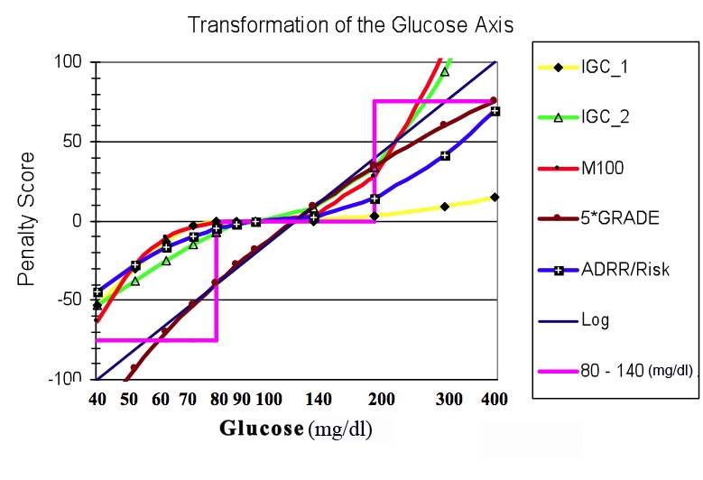
Comparison of several types of transformations of the glucose scale. Abscissa, glucose on semilogarithmic scale from 40 to 400 mg/dl; ordinate, transformations, including logarithmic transform with an arbitrary linear scaling factor, G' = 200*log(glucose/126.5) (black straight line, no data points); use of a criterion that glucose should be in the range 80 to 200 mg/dl (pink step function); IGC1 (yellow, black diamonds) using parameters LLTR = 80, ULTR = 140, b = 2.0, a = 1.1, and c = d = 30; IGC₂, (green, open triangles) using parameters LLTR = ULTR = 100 mg/dl (a target level of 100), b = 1.8, a = 1.5, c = d = 30; Schlichtkrull M_R index with R = 100 mg/dl (M₁₀₀, red curve with black closed circles), Kovatchev and colleagues' HBGI and LBGI transformations (blue curve with closed black squares with superimposed white plus sign), and Hill and coworkers' GRADE score transformation (brown curve with superimposed closed brown circles) multiplied by a constant scaling factor of five to facilitate comparison with the other transformations. Of the transformations included here, the GRADE transformation most closely approximates a simple log transformation.

The curves corresponding to these transformations are closely clustered together, especially in the range where the majority of glucose values are likely to fall, e.g., 60 to 250 mg/dl (Figure 2). This explains why these criteria give very similar, highly correlated results, as was observed when each of these transformations was applied to clinical studies so as to obtain an overall average measure of quality of glycemic control after an intervention.^9,13–15

Discussion

The present study proposes that use of a logarithmic scale (alternatively designated as a semilogarithmic scale) for glucose can potentially make it easier for physicians and patients to appreciate fluctuations, patterns, and excursions in the hypoglycemic and euglycemic ranges, without sacrificing the ability to appreciate changes in the hyperglycemic range. Log scales for glucose have been used previously, in the context of the intravenous glucose tolerance test, to facilitate the estimate of the glucose disappearance rate constant.¹⁶ However, a literature search failed to identify previous use of log(glucose) for the display of SMBG or CGM data in routine clinical practice. Use of semilogarithmic scales are very common in medicine and the sciences in general. Many kinds of clinical laboratory data are more nearly “log normal” in distribution than “normal” (Gaussian) in distribution, so it is a routine practice in many scientific studies and statistical analyses to display data using a semilogarithmic scale or to utilize a log transform. In view of the potential advantages of a log scale for glucose, it would be desirable to have an option to display graphs in this format in programs for routine display of SMBG and CGM data. It would be important to retain the option to utilize linear scales, because most users of this software are accustomed to use of linear scales. However, the individual user should have the option to select the scale to be used as a routine or “default approach.”

It might also be desirable to provide the user with options to use any one of the kinds of transformations described here (e.g., 1–10 in Methods) to display the data or to perform statistical analyses. For example, when computing standard deviations, or a more detailed analysis of variance,^9,13–15 it may be desirable to use one or another of these transformations. Multiple large-scale data sets obtained from multiple subjects have been examined using several criteria for symmetry and Gaussianness of the distribution of glucose values, and it was found that, for many patients, Gaussianness is best achieved with use of a modified log transform, log(glucose + c), where c is a small constant that often falls in the range from 15 to 30 mg/dl. In contrast, use of a simple log transform (with c = 0) often results in an asymmetrical distribution, tailing off to the left, corresponding to a negative skew or skewness.

Use of these transformations can provide a number of advantages: improved symmetry and Gaussianness of the distribution of glucose values, increased emphasis on the hypoglycemic range, and reduction of the correlation of mean glucose and the standard deviation of glucose commonly observed when using the original (untransformed) glucose data for analysis of data from multiple individuals.

A logarithmic scale can be applied to glucose values equally well whether they are expressed in units of mg/dl or mmol/liter. If desired, one can show glucose expressed in mg/dl on one of the vertical axes and glucose expressed in mmol/liter on the other vertical axis (Figures 1C and 1D). Alternative transformations (e.g., M₁₀₀, IGC, LBGI/HBGI, GRADE as shown in Figure 2) are also expected to be useful when calculating the variance or standard deviation of the glucose distribution, since these transformations were designed so that the transformed values would be more closely related to the potentially deleterious clinical risks than the original (linear) scale for glucose.

Glucose fluctuations in the hyperglycemic range are often so large and dominating that it is easy to overlook a few values in the hypoglycemic range, even if they occur consistently at about the same time of day, within a localized range of dates or on a particular day of the week. The author's experience suggests that it is not uncommon for physicians to fail to detect significant patterns and features either when using graphic displays or inspection of tabular (logbook) data. This problem is compounded by the fact that the patient may present to an office visit with 3 months of data, which may need to be analyzed within a period of 2 or 3 min, at best.

There are few, if any, studies of the ability of physicians to interpret graphic displays, e.g., of vital signs, flowcharts, and laboratory data, in terms of accuracy, sensitivity for detection of various features, reproducibility, and speed. It is possible that, with appropriate training, many or most physicians might be able to interpret the graphic displays using a linear scale much better than they had been previously. The premise of the present report is that, by displaying glucose on a log scale, it would be possible for physicians to improve their ability to analyze and interpret these graphic displays with little or no additional training. How can one objectively evaluate whether the new type of displays, as described here and in related studies describing new methods for graphic displays of glucose data,^17,18 result in significant improvement in the effectiveness of the computer analysis of SMBG and CGM data? One can use empirical field evaluation and cognitive laboratory studies.

Empirical Field Evaluation

One or more of the developers of software for routine analysis of SMBG and CGM data could include an option to provide graphs using a logarithmic scale for glucose. One could then utilize a survey or questionnaire to assess whether the users like the method and whether they plan to use it in the future, along with their reasons for their response. However, a much better criterion for evaluating whether new methods are useful would be to monitor the percentage of clinicians, patients, and other users who utilize graphs with logarithmic scales and the relative frequency of use compared with a simple linear scale. These approaches would capture the information needed to answer the question of whether potential users like the method and, more importantly and objectively, whether they actually use it.

Cognitive Laboratory Studies

It would be desirable to perform a cognitive laboratory study involving a reasonable number (perhaps 25) of physicians, other members of diabetes management teams, and patients. Such a study would involve display of a series of graphic displays from several case studies—using both linear and log scales—and asking the subjects to identify and prioritize the problems illustrated by each case (e.g., hyperglycemia, hypoglycemia, variability, inadequate monitoring, or combinations of these). Such a study might involve 25 subjects × 10 case studies × 2 types of displays × 2 types of graphs (glucose by date, glucose by time of day) or 1000 analyses. That study would need to be repeated for different durations of display of each graph, e.g., 5, 10, and 15 s, resulting in a total of 3000 displays. The study becomes more complicated because the subjects may “learn” as they are viewing the 10 × 2 × 2 × 3 = 120 showings. The study should be videotaped to secure objective data that can be reviewed, or it could be computer administered so that one could capture the length of time that the subject requires to make decisions about the types of patterns or problems for each case study. This entire process could be repeated separately for data from SMBG or from CGM, for different densities of data for SMBG (e.g., once per day versus six times per day), and for glucose time series of different durations. So this simple little study is really large and complex and would require institutional review board approval, and substantially delay the reporting of this modest little proposal. The problem of possible (and likely) “learning” during the study would be particularly challenging but could be addressed using randomization of the order of presentation of the displays or by means of a crossover study. These kinds of studies could also evaluate the effectiveness of tabular displays such as logbooks and electronic displays simulating logbooks. Indeed, they would be helpful for evaluation of the effectiveness and user-friendliness of all of the components of displays of glucose, medications, diet, exercise, and related data as captured in routine analyses of SMBG, CGM and CSII data. In view of the size, scope, and costs of these types of studies, it was not possible to include them in the present report.

Conclusions

Current methods for display of glucose data generally give insufficient emphasis and inadequate resolution to the hypoglycemic range. The simple expedient of plotting glucose on semilogarithmic graph paper or use of the numerical (digital) equivalent, log₁₀(glucose), expands the relative range of the hypoglycemic data by a factor of three. This approach is applicable to graphs of glucose by date, time of day, or day of the week and is applicable to displays of either CGM or SMBG data. The log scale imparts better symmetry and Gaussianness of the glucose distribution, which can facilitate statistical analyses. Several alternative transformations are available and may be useful in selected circumstances and applications. However, the simple log transform appears to be sufficient for most purposes to facilitate graphic analysis and interpretation of glucose data. Studies to evaluate the effectiveness of this and other methods for display of SMBG and CGM data have been designed and planned.

Abbreviations

CGM

continuous glucose monitoring

CSII

continuous subcutaneous insulin infusion

HBGI

high blood glucose index

IGC

index of glycemic control

LBGI

low blood glucose index

LLTR

lower limit of the target range

SMBG

self-monitoring of blood glucose

ULTR

upper limit of the target range

References

- 1.The Diabetes Control and Complications Trial Research Group. Hypoglycemia in the Diabetes Control and Complications Trial. Diabetes. 1997;46(2):271–286. [PubMed] [Google Scholar]
- 2.Skyler JS, Bergenstal R, Bonow RO, Buse J, Deedwania P, Gale EA, Howard BV, Kirkman MS, Kosiborod M, Reaven P, Sherwin RS. American Diabetes Association, American College of Cardiology Foundation, American Heart Association. Intensive glycemic control and the prevention of cardiovascular events: implications of the ACCORD, ADVANCE, and VA Diabetes Trials: a position statement of the American Diabetes Association and a Scientific Statement of the American College of Cardiology Foundation and the American Heart Association. J Am Coll Cardiol. 2009;53(3):298–304. doi: 10.1016/j.jacc.2008.10.008. [DOI] [PubMed] [Google Scholar]
- 3.American Diabetes Association. Veterans Administration Diabetes Trial. http://www.diabetesconnect.org/storetemplate/CVDPackage.aspx Accessed September 23, 2009.
- 4.Garg S, Zisser H, Schwartz S, Bailey T, Kaplan R, Ellis S, Jovanovic L. Improvement in glycemic excursions with a trans-cutaneous, real-time continuous glucose sensor: a randomized controlled trial. Diabetes Care. 2006;29(1):44–50. doi: 10.2337/diacare.29.01.06.dc05-1686. [DOI] [PubMed] [Google Scholar]
- 5.Garg S, Jovanovic L. Relationship of fasting and hourly blood glucose levels to HbA1c values: safety, accuracy, and improvements in glucose profiles obtained using a 7-day continuous glucose sensor. Diabetes Care. 2006;29(12):2644–2649. doi: 10.2337/dc06-1361. [DOI] [PubMed] [Google Scholar]
- 6.Bailey TS, Zisser HC, Garg SK. Reduction in hemoglobin A1C with real-time continuous glucose monitoring: results from a 12-week observational study. Diabetes Technol Ther. 2007;9(3):203–210. doi: 10.1089/dia.2007.0205. [DOI] [PubMed] [Google Scholar]
- 7.Schlichtkrull J, Munck O, Jersild M. The M-valve, an index of blood-sugar control in diabetics. Acta Med Scand. 1965;177:95–102. doi: 10.1111/j.0954-6820.1965.tb01810.x. [DOI] [PubMed] [Google Scholar]
- 8.Rodbard D. Diabetes Technology Meeting. San Francisco: CA; 2005. Nov, Improved methods for calculating a “figure of merit” for blood glucose monitoring data. [Google Scholar]
- 9.Rodbard D. Interpretation of continuous glucose monitoring data: glycemic variability and quality of glycemic control. Diabetes Technol Ther. 2009;11(Suppl 1):S55–S67. doi: 10.1089/dia.2008.0132. [DOI] [PubMed] [Google Scholar]
- 10.Kovatchev BP, Cox DJ, Gonder-Frederick LA, Young-Hyman D, Schlundt D, Clarke W. Assessment of risk for severe hypoglycemia among adults with IDDM: validation of the low blood glucose index. Diabetes Care. 1998;21(11):1870–1875. doi: 10.2337/diacare.21.11.1870. [DOI] [PubMed] [Google Scholar]
- 11.Kovatchev BP, Otto E, Cox D, Gonder-Frederick L, Clarke W. Evaluation of a new measure of blood glucose variability in diabetes. Diabetes Care. 2006;29(11):2433–2438. doi: 10.2337/dc06-1085. [DOI] [PubMed] [Google Scholar]
- 12.Hill NR, Hindmarsh PC, Stevens RJ, Stratton IM, Levy JC, Matthews DR. A method for assessing quality of control from glucose profiles. Diabet Med. 2007;24(7):753–758. doi: 10.1111/j.1464-5491.2007.02119.x. [DOI] [PubMed] [Google Scholar]
- 13.Rodbard D. New and improved methods to characterize glycemic variability using continuous glucose monitoring. Diabetes Technol Ther. 2009;11(9):551–565. doi: 10.1089/dia.2009.0015. [DOI] [PubMed] [Google Scholar]
- 14.Rodbard D, Bailey T, Jovanovic L, Zisser H, Kaplan R, Garg S. Reduced glycemic variability with the use of real-time continuous glucose monitoring. Diabetes Technol Ther. 2009;11(11):717–723. doi: 10.1089/dia.2009.0077. [DOI] [PubMed] [Google Scholar]
- 15.Rodbard D, Jovanovic L, Garg S. Impact of continuous glucose monitoring in patients with type 1 diabetes using multiple daily injections versus insulin pump. Diabetes Technol Ther. 2009;11(12) doi: 10.1089/dia.2009.0078. In press. [DOI] [PubMed] [Google Scholar]
- 16.Rosenqvist U, Licko V, Karam JH. Evaluation of a “true” fractional removal rate of glucose in man by bolus and simulated-ramp increase of glucose. Diabetes. 1976;25(7):580–585. doi: 10.2337/diab.25.7.580. [DOI] [PubMed] [Google Scholar]
- 17.Rodbard D. New approaches to display of self-monitoring of blood glucose data. J Diabetes Sci Technol. 2009;3(5):1121–1127. doi: 10.1177/193229680900300515. [DOI] [PMC free article] [PubMed] [Google Scholar]
- 18.Rodbard D. Display of glucose distributions by date, time of day, and day of week: new and improved methods. J Diabetes Sci Technol. 2009;3(6):1388–1394. doi: 10.1177/193229680900300619. [DOI] [PMC free article] [PubMed] [Google Scholar]