Real-time calculation of a limiting form of the Renyi entropy applied to detection of subtle changes in scattering architecture

Abstract

Previously a new method for ultrasound signal characterization using entropy H_f was reported, and it was demonstrated that in certain settings, further improvements in signal characterization could be obtained by generalizing to Renyi entropy-based signal characterization I_f(r) with values of r near 2 (specifically r=1.99) [M. S. Hughes et al., J. Acoust. Soc. Am. 125, 3141–3145 (2009)]. It was speculated that further improvements in sensitivity might be realized at the limit r→2. At that time, such investigation was not feasible due to excessive computational time required to calculate I_f(r) near this limit. In this paper, an asymptotic expression for the limiting behavior of I_f(r) as r→2 is derived and used to present results analogous to those obtained with I_f(1.99). Moreover, the limiting form I_f,∞ is computable directly from the experimentally measured waveform f(t) by an algorithm that is suitable for real-time calculation and implementation.

INTRODUCTION

In an earlier paper1 we reported on the application of Renyi entropy I_f(r), which is defined for all r<2 (r is roughly a reciprocal “temperature”), for the detection of changes in backscattered radio frequency (rf) ultrasound arising from the accumulation of targeted nanoparticles in the neovasculature in the insonified region of a tumor. That study was motivated by the observation that acoustic characterization of sparse collections of targeted perfluorocarbon nanoparticles presented challenges that might require the application of novel types of signal processing.2 We were able to show that signal processing based on a “moving window” H_f analysis [see Eq. 7] could detect accumulation of tissue-targeted nanoparticles 30 min following nanoparticle injection. The signal energy, defined as the sum of squares over the same moving window, was unable to distinguish measurements made at any time during the 1 h experiment (as was conventional B-mode imaging). Subsequently we determined that moving window I_f(r) analysis, with r=1.99, could distinguish the difference in backscatter measured at 0 and 15 min. Reduction in the accumulation time required to reach detectability from 30 to 15 min is clearly of significance: potentially reducing both patient discomfort and increasing clinical throughput. Moreover, although the computational effort to obtain the result precluded its clinical application with currently available equipment, the study raised the possibility of further sensitivity improvements by using values of r closer to the limiting value of 2, where I_f(r) approaches infinity. The purpose of the current study is to investigate the behavior of I_f(r) as r→2 by extracting its asymptotic form. While this involves use of the second derivatives of f(t) at its critical points, which can be expected to increase noise in the processing chain output, surprisingly the resulting signal processing scheme does not sacrifice sensitivity. Moreover, the operation count in this approach is lower than that used to produce the signal envelope, which currently is the standard for real-time ultrasonic imaging display, thus demonstrating its suitability for implementation in a real-time imaging system to facilitate detection of molecular epitopes associated with neovasculature in a growing tumor. As our technique is based on moving window analysis of digitized rf, which requires some sacrifice in spatial resolution, clinical implementation of entropy detection would probably follow the same approach currently employed in Doppler “imaging” systems, where the conventional B-mode image is color-coded according to the blood cell velocity to present a combined B-mode∕velocity image; similarly, a B-mode∕entropy image could be made as well.

APPROACH

All results in this study were obtained using the density function w_f(y) of the continuous function y=f(t), assumed to underlie the sampled rf data. Subsequently, w_f(y) was used to compute the entropy I_f(r). As described in previous studies w_f(y) corresponds to the density functions used in statistical signal processing.1 In contradistinction to statistical signal processing, where f(t) is a random function, and often nowhere differentiable, we assume that the noise levels in our apparatus are low enough so that with sufficient signal averaging, noise may be eliminated, or at least reduced to a low enough level, that derivatives of f(t) may be accurately computed. From these derivatives the density function w_f(y) may be computed,1 which then facilitates calculation of the quantities typically discussed in statistical signal processing (e.g., mean values, variances, and covariances).3, 4, 5 However, in that environment, the density function is usually assumed to be continuous, infinitely differentiable, and to approach zero at infinity. In our case w_f(y) is not so well-behaved and has (integrable) singularities. While this renders calculation of the density function more difficult, applications of entropy imaging based on w_f(y) have shown the cost to be justified in terms of increased sensitivity to subtle changes in scattering architecture that are often undetected by more conventional imaging.

We use the same conventions as in previous studies so that

$$w_f\left(y\right)=\sum _{k=1}^N\mid g_k^{\prime }\left(y\right)\mid ,$$ (1)

where N is the number of laps [regions of monotonicity of f(t)], g_k(y) is the inverse of f(t) in the kth-lap, and if y is not in the range of f(t) in the kth-lap, $g_k^{\prime }\left(y\right)$ is taken to be 0.

We also assume that all experimental waveforms f(t) have a Taylor series expansion valid in the domain [0,1]. Then near a time t_k such that f^′(t_k)=0,

$$y=f\left(t\right)=f\left(t_k\right)+\frac{1}{2!}{f}^{″}\left(t_k\right){\left(t-t_k\right)}^2+\cdots ,$$ (2)

where t_k is a lap boundary. On the left side of this point Eq. 2 may be truncated to second order and inverted to obtain

$$g_k\left(y\right)\sim t_k\pm \sqrt{2\left(y-f\left(t_k\right)\right)∕f^{″}\left(t_k\right)},$$ (3)

with

$$\mid g_k^{\prime }\left(y\right)\mid \sim 1∕\sqrt{2f^{″}\left(t_k\right)\left(y-f\left(t_k\right)\right)}.$$ (4)

The contribution to w_f(y) from the right side of the lap boundary, from g_k+1(y), is the same, so that the overall contribution to w_f(y) coming from the time interval around t_k is

$$\mid g_k^{\prime }\left(y\right)\mid \sim \sqrt{2∕\left(f^{″}\left(t_k\right)\left(y-f\left(t_k\right)\right)\right)},$$ (5)

for 0<f(t_k)−y⪡1 for a maximum at f(t_k) and 0<y−f(t_k)⪡1 for a minimum. Thus, w_f(y) has only a square root singularity (we have assumed that t_k is interior to the interval [0,1]; if not, then the contributions to w_f come from only the left or the right). If, additionally, f^″(t_k)=0, then the square root singularity in Eq. 4 will become a cube-root singularity, and so on, so that the density functions we consider will have only integrable algebraic singularities.

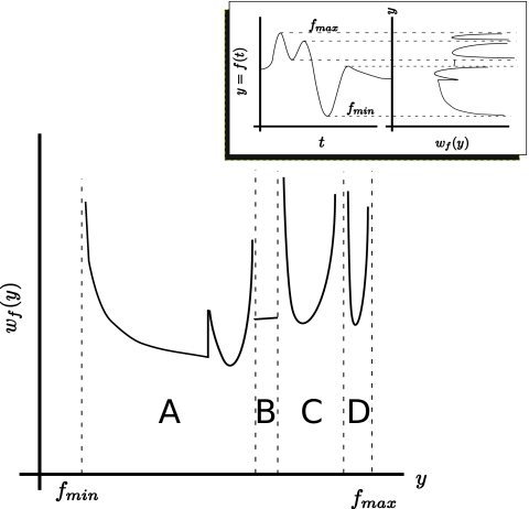
Figure 1 shows a typical waveform (inset) and its associated density function, which may be divided into four different regions, A–D, separated by singularities (dashed lines) corresponding to the critical points of f(t). In general, three types of behavior are possible in w_f(y): continuous, finite jump discontinuity, and integrable singularity. In region A, there are two singularities and a finite jump discontinuity. In region B, w_f(y) is continuous. In C and D, there are singularities at the region boundaries. This figure shows that the density functions possess significantly different attributes from those usually considered in statistical signal processing. To compare the current approach with that usually taken in discussions of “random variable theory,” we point out that a “random variable,” usually denoted X(t) [instead of our f(t)] is nothing more or less than a Lebesgue measurable function. In many applications of random variable theory, X(t) is everywhere continuous but nowhere differentiable (e.g., the Brownian motion), and various means are devised to estimate its probability density function. In the current investigation, it is not necessary to estimate w_f(y) by these means since we may calculate it from f(t). However, as f(t) is assumed to be Lebesgue measurable, it is, in the strictly formal sense, also a random variable, and w_f(y) is its probability density function. As we are investigating a subset of random variables, where it happens that the probability density function may be calculated from the random variable itself, we will carefully refrain from using this term, since it will only raise associations with the reader’s mind that are misleading in the current context.

Figure 1.

Plot of a typical density function w_f(y) employed in our study. Inset shows a time-domain waveform f(t) with five critical points (left) and their relationship to the singularities of the associated density function w_f(y) (right).

The mathematical characteristics of the singularities of w_f(y) are important in order to guarantee the existence of the following integral on which we base our analysis of signals in this study:

$$I_f\left(r\right)=\frac{1}{1-r}\text{log}\left[{\int }_{f_{\text{min}}}^{f_{\text{max}}}{w}_f{\left(y\right)}^{r}dy\right],$$ (6)

which is known as the Renyi entropy.6 It is similar to the partition function in statistical mechanics with the parameter r playing the role of an “artificial” reciprocal temperature1, 7 (unrelated to the actual physical temperature in the scattering region); moreover, I_f(r)→−H_f, as r→1, using L’Hôpital’s rule, so that I_f is a generalization of H_f as follows:

$$H_f={\int }_{f_{\text{min}}}^{f_{\text{max}}}{w}_f\left(y\right)\text{log}{w}_f\left(y\right)dy.$$ (7)

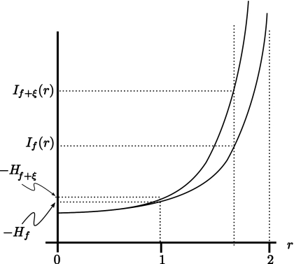
Previous studies have shown that this quantity can be more sensitive to subtle changes in scattering architecture than are more commonly used energy-based measures,2 with subsequent studies demonstrating further sensitivity improvements using I_f at the suitable value of r.1 For the density functions w_f(y) encountered in our study, I_f(r) is undefined for r≥2, since as r→2⁻, the integral appearing in Eq. 6 will grow without bound due to the singularities in the density function w_f(y) described in Eq. 5. The behavior as r→2 is dominated by contributions from these singularities, all of which correspond to critical points of f(t). This behavior is shown in Fig. 2. Moreover, as shown in the figure, it is possible that two slightly different functions, f(t) and f(t)+ξ(t), where ξ is small, may have entropies, H_f and H_f+ξ, that are close, as shown, but whose Renyi entropies, I_f(r) and I_f+ξ(r), diverge as r→2. Previous studies have shown that this can happen in practice.1 However, these results left open the possibility of further sensitivity gains. The purpose of the present study is to investigate the possibility of obtaining further sensitivity improvements by pushing toward this limit. As described in the Appendix0, the asymptotic form of I_f(r) as r→2 is given by

$$I_{f,\infty }=\text{log}\left[\sum _{\left\{t_k\mid f^{\prime }\left(t_k\right)=0\right\}}\frac{1}{\mid f^{″}\left(t_k\right)\mid }\right].$$ (8)

We will use this quantity to generate the images presented in the current study.

Figure 2.

Plots of I_f(r) and I_f+ξ(r) (left) showing that while I_f(1)=−H_f and I_f+ξ(1)=−H_f+ξ may be close, I_f(r) and I_f+ξ(r) diverge as r→2.

MATERIALS AND METHODS

Numerical computation of I_f,∞

Calculation of I_f,∞ via Eq. 8 is accomplished by fitting a cubic spline to the experimentally acquired data array using a well-known algorithm, which returns the second derivative of the cubic spline (in an array having the same length as the experimental data) and initializes data structures suitable for rapid computation of its first derivative.8 Subsequently, an array of corresponding first derivatives is computed and used to bracket the critical points of the spline (i.e., the zero crossings). Linear interpolation is then used to estimate the exact location of the bracketed zero crossings in order to obtain an algorithm suitable for real-time implementation in a medical imaging system. The total operation count is of order N_σ, where N_σ is the number of points processed, and is more than four orders of magnitude faster than the operation count 16 384N_σ required to compute I_f(r) used in our previous study.1 For comparison, we also note that the operation count required to produce the envelope of the same number of points (i.e., to produce a conventional B-mode image) would be of order N_σ log(N_σ) since computation of the envelope requires use of the fast Fourier transform; for the value of N_σ=512 used in our study below, this represents an increase in processing speed of roughly ninefold.

Simulations

The convergence properties, stability in the presence of noise, and effects of quantization error and sampling rate have been extensively evaluated using simulated data. Several types of waveforms have been investigated: Gaussian and parabolic waveforms, for which the exact value of I_f,∞ may be computed and linear combinations of exponentially damped sine waves that qualitatively resemble backscattered ultrasonic waveforms. Several carefully chosen example simulations illustrate guidelines for application of our algorithm in order to avoid potential artifacts produced by experimental factors.

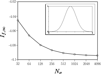
The first of these is Fig. 3, which shows a plot of I_f,∞ for a noise-free Gaussian pulse f(t)=e^{−30(t−0.5)2} for values of N_σ ranging from 32, 64, 128,…, 8192. Even at N_σ=32 the estimated value of I_f,∞ is within 1% of the exact value of log[1∕60]=−4.094. For moving window analysis of experimental data, N_σ is the length of the moving window. Choosing its length requires making trade-offs between sensitivity (smaller N_σ implying loss of sensitivity, but increased spatial resolution), noise level (smaller N_σ implying increased noise, but increased spatial resolution), and spatial resolution.

Figure 3.

Simulation for a noise-free Gaussian pulse showing the dependence of I_f,∞ on the number of sampled points N_σ.

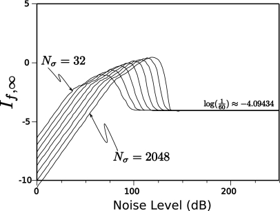
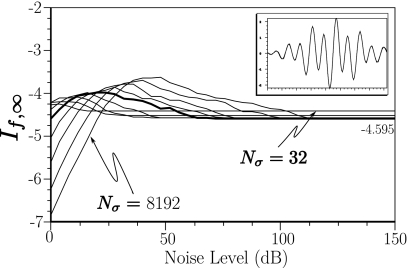
However, noise can have a significant effect on the calculation of I_f,∞. Figure 4 illustrates the impact of noise on the Gaussian pulse (f(t)=e^{−30(t−0.5)2}) that was just discussed. As N_σ ranges from 32, 64, 128,…, 8192 and noise levels ranges from 0 to 150 dB, the calculated value of I_f,∞ can vary by over 100% of its actual value. Eventually, as N_σ increases and the noise level drops, our algorithm converges to a stable value. However, as the plots indicate, the noise requirements for a single peak function such as the Gaussian peak are quite stringent, being greater than 100 dB to obtain 10% accuracy.

Figure 4.

Simulation for a Gaussian pulse showing the dependence of I_f,∞ on the number of sampled points N_σ and noise level.

These requirements are less stringent if f(t) has several critical points. An example is shown in Fig. 5, which plots I_f,∞ for values of N_σ ranging from 32, 64, 128,…, 2048, and for noise levels ranging from 0 to 150 dB for the Gaussian modulated pulse f(t)=e^{−10(t−0.5)2} sin(20π(t−0.5))+0.7 sin(20π(t−0.5))+0.7 sin(10π(t−0.5)). As the plots indicate the noise requirements for a multipeak peak waveform f(t) are far less stringent with 87% accuracy being obtained at about 20 dB noise level for N_σ=512 (plotted using a heavier line in the plot family since these parameters match values used in the experimental portion of our study).

Figure 5.

Simulation for an unquantized Gaussian modulated pulse showing the dependence on the number of sampled points N_σ and noise level.

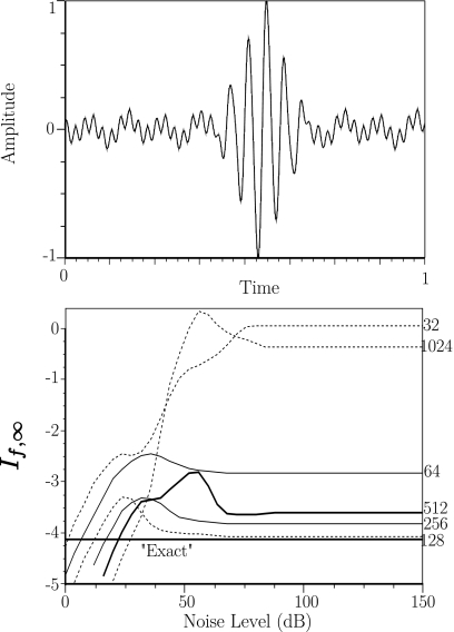
Figure 6 shows a plot of I_f,∞ for values of N_σ ranging from 32, 64, 128,…, 8192 for noise levels ranging from 0 to 150 dB for the simulated pulse f(t)=e^{−150(t−0.55)2} sin(40π(t−0.55))+0.7 sin(80π(t−0.55))+0.7 sin(20π(t−0.55))+0.03 sin(10π(t−0.55)). The “exact” answer is −4.149 073, found by running our algorithm with noise level set to zero, no quantization error, and N_σ=8192, and is also shown in the plot. The corresponding values of N_σ are indicated on the right side of the figure. For values of N_σ≤512 the error is less than 13%. We also note that for larger values of N_σ and lower levels of noise, our algorithm diverges with I_f,∞ becoming large and positive. This occurs only in quantized simulations and is the result of the long perfectly flat segments in the quantized data. This is an easily detected fault and, since the I_f,∞ images used in our experimental study had pixel values of approximately 7 bits∕symbol in magnitude on the regions used to estimate accumulation of targeted nanoparticles, can be ruled out as a possible artifact in our study.

Figure 6.

Top panel: the simulated backscatter signal described in the text. Bottom panel: plot showing the dependence of I_f,∞ on the number of sampled points N_σ and noise level at 8-bit quantization. The heavy black line labeled “Exact” is at 4.149, the limiting value of I_f,∞ obtained from our algorithm in the unquantized, noise-free case with N_σ=8192.

Nanoparticles for molecular imaging

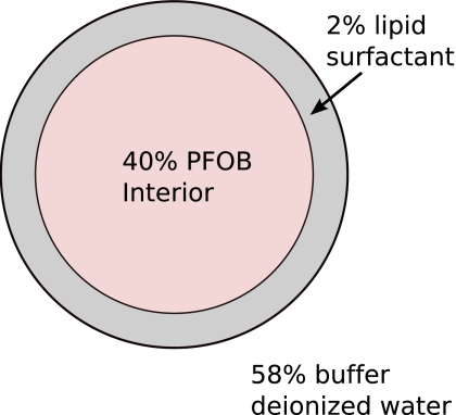
A cross-section of the spherical liquid nanoparticles used in our study is diagramed in Fig. 7. For in vivo imaging we formulated nanoparticles targeted to α_vβ₃-integrins of neovascularity in cancer by incorporating an “Arg-Gly-Asp” mimetic binding ligand into the lipid layer. Methods developed in our laboratories were used to prepare perfluorocarbon (perfluorooctylbromide, which remains in a liquid state at body temperature and at the acoustic pressures used in this study9) emulsions encapsulated by a lipid-surfactant monolayer.10, 11 The nominal sizes for each formulation were measured with a submicron particle analyzer (Malvern Zetasizer, Malvern Instruments). Particle diameter was measured at 200±30 nm.

Figure 7.

A cross-sectional diagram of the nanoparticles used in our study.

Animal model

The study was performed according to an approved animal protocol and in compliance with guidelines of the Washington University Institutional Animal Care and Use Committee.

The model used is the transgenic K14-HPV16 mouse in which the ears typically exhibit squamous metaplasia, a precancerous condition, associated with abundant neovasculature that expresses the α_vβ₃-integrin. Eight of these transgenic mice12, 13 were treated with 1.0 mg∕kg intravenous of either α_vβ₃-targeted nanoparticles (n=4) or untargeted nanoparticles (n=4) and imaged dynamically for 1 h using a research ultrasound imager (Vevo 660 40 MHz probe) modified to store digitized rf waveforms acquired at 0, 15, 30, and 60 min after injection of nanoparticles. In both targeted and untargeted cases, the mouse was placed on a heated platform maintained at 37 °C, and anesthesia was administered continuously with isoflurane gas (0.5%).

Ultrasonic data acquisition

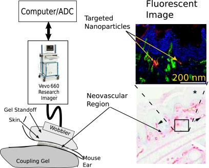
A diagram of our apparatus is shown in Fig. 8. rf data were acquired with a research ultrasound system (Vevo 660, Visualsonics, Toronto, Canada), with an analog port and a sync port to permit digitization. The tumor was imaged with a 40 MHz single element “wobbler” probe and the rf data corresponding to single frames were stored on a hard disk for later off-line analysis. The frames (acquired at a rate of 40 Hz) consisted of 384 lines of 4096 8-bit words acquired at a sampling rate of 500 MHz using a Gage CS82G digitizer card (connected to the analog-out and sync ports of the Vevo) in a controller PC. Each frame corresponds spatially to a region 0.8 cm wide and 0.3 cm deep.

Figure 8.

A diagram of the apparatus used to acquire rf data backscattered from K14-HPV16 transgenic mouse ears in vivo together with a histologically stained section of the ear indicating portions where α_vβ₃-targeted nanoparticles could adhere and a fluorescent image demonstrating presence of targeted nanoparticles.

The wobbler transducer used in this study is highly focused (3 mm in diameter) with a focal length of 6 mm and a theoretical spot size of 80×1100 μm (lateral beam width×depth of field at −6 dB), so that the imager is most sensitive to changes occurring in the region swept out by the focal zone as the transducer is “wobbled.” Accordingly, a gel standoff was used, as shown in Fig. 8, so that this region would contain the mouse ear.

A close-up view showing the placement of transducer, gel standoff, and mouse ear is shown in the bottom of the figure. Superposed on the diagram is a B-mode gray scale image (i.e., logarithm of the analytic signal magnitude). Labels indicate the location of skin (top of image insert), the structural cartilage in the middle of the ear, and a short distance below this, the echo from the skin at the bottom of the ear. Directly above this is an image of a histological specimen extracted from a K14-HPV16 transgenic mouse model that has been magnified 20 times to permit better assessment of the thickness and architecture of the sites where α_vβ₃-targeted nanoparticle might attach (red by β₃ staining). Skin and tumor are both visible in the image. On either side of the cartilage (center band in image), extending to the dermal-epidermal junction, is the stroma. It is filled with neoangiogenic microvessels. These microvessels are also decorated with α_vβ₃ nanoparticles as indicated by the fluorescent image (labeled, in the upper right of the figure) of a bisected ear from an α_vβ₃-injected K14-HPV16 transgenic mouse. It is in this region that the α_vβ₃-targeted nanoparticles are expected to accumulate, as indicated by the presence of red β₃ stain in the magnified image of a histological specimen also shown in the image.

Ultrasonic data processing

Each of the 384 rf lines in the data was first up-sampled from 4096 to 8192 points, using a cubic spline fit to the original data set in order to improve the stability of the thermodynamic receiver algorithms. A by-product of this “order N_σ” algorithm is simultaneous output of a corresponding array of second derivative values of the fit function.8 Next, a moving window analysis was performed on the second derivative data set, using Eq. 8 to compute I_f,∞, by moving a rectangular window (512 points long, 0.512 μs) in 0.064 μs steps (64 points), resulting in 121 window positions within the output data set. This produced an image for each time point in the experiment. The window length was chosen to match that used in previous studies;1, 2 it corresponds to the heavy black curve shown in Fig. 6. Analyses were also performed using window lengths of 256 (0.256 μs) and 128 points (0.256 μs). While they also produced statistically significant changes in I_f,∞ versus time, post-injection, the resulting I_f,∞ versus time curves were noisier, and required 1 h, post-injection, to exhibit statistically significant changes. As discussed previously, the optimum choice of window length requires trade-offs between sensitivity, noise level, and spatial resolution. In Sec. 4 we discuss the 512 point moving window length results since they correspond most closely to previous results, which were supported by independent histological results,1, 2 and produced images with sufficient spatial resolution to indentify relevant anatomical features in the mouse ear. Additionally, a major goal of this study was to assess the numerical stability of the algorithm, which is based on the second derivative of an experimentally measured data set, and thus contaminated by noise. Ordinarily, estimation of just the first derivative is difficult. However, in our application, the effects of noise might be mitigated by two factors: The second derivative is obtained from a global fit to the data, and it appears in the denominator of the expression for receiver output so that values having large error are likely to make small contributions to the sum appearing in Eq. 8.

Image processing

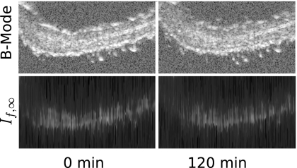
All rf data were processed off-line to reconstruct I_f,∞ images. Total analysis time using the new algorithm was less than 5 min on an eight core desktop computer [compared to the roughly week-long time required to execute the I_f(1.99) analysis on a cluster of just over 20 computers that was reported previously1]. A representative set of these images is shown in the bottom row of Fig. 9. For comparison, the top row shows conventional B-mode images, i.e., logarithm of the signal envelope. The left columns show images constructed from the rf data sets acquired 0 min after injection while the right column shows the images constructed from data acquired 120 min post-injection. The look-up-table of the entropy images have been inverted to produce a display in which pixels corresponding to tissue are brighter than surrounding pixels, in order to facilitate comparison with the conventional images. As expected, the conventional images exhibit higher spatial resolution compared with the I_f,∞ images, which employ a moving window in their construction. While the window is discernible in the entropy images, it is not a cause of major concern since our goal is automatic quantitative detection of changes in scattering architecture in the physical region represented by the image. As may be seen from the figure, the bright regions in I_f,∞ and conventional images are correlated. Moreover, as time passes from 0 to 120 min, both rows of images show a reduction in contrast between tissue of the ear (bright regions) and darker background (corresponding to the gel couplant). In the I_f,∞ images this corresponds to an increase in I_f,∞. As discussed below this effect is consistently observed in all I_f,∞ images from the group of K14-HPV16 transgenic mice injected with α_vβ₃-targeted nanoparticles, and it is not observed in I_f,∞ images from any of the control groups. As stated in previous publications, there are no statistically significant changes in signal energy images in any of the groups studied.2

Figure 9.

Top row: conventional B-mode images at 0 min (left), and after injection of α_vβ₃-targeted nanoparticles (right). Bottom row: corresponding I_f,∞ images.

Subsequently, a histogram of pixel values for the composite of the 0, 15, 30, and 60 min images was computed as described in previous papers.1, 2 Image segmentation of each type of image, at each time point in the experiment, was then performed automatically using its corresponding histogram according to the following threshold criterion: The lowest 7% of pixel values were classified as “targeted” tissue, while the remaining were classified as “untargeted” (histogram analysis was also performed using 90% and 87% thresholds, with 93% having the best statistical separation between time points). The mean value of pixels classified as targeted was computed at each time post-injection.

RESULTS AND DISCUSSION

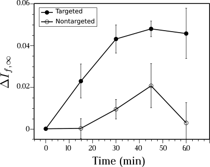
The results obtained after injection of targeted nanoparticles and nontargeted nanoparticles by I_f,∞ receiver are shown in Fig. 10. Both curves show the time evolution of the change (relative to 0 min) in mean value of receiver output in the enhanced regions of images obtained from the four animals in the targeted and the four animals in the nontargeted groups. Standard error bars are shown with each point. At 15 min the change in mean value of I_f,∞ is more than two standard errors from zero, implying statistical significance at the 95% level. There is no statistically significant change in image brightness for the nontargeted nanoparticles’ group. As the results show, the algorithm for computation of I_f,∞ is stable in the presence of experimental noise.

Figure 10.

I_f,∞ image enhancement, i.e., change relative to 0 min, obtained after injection of α_vβ₃-targeted nanoparticles (closed circles) and nontargeted nanoparticles (open circles) into four K14-HPV16 transgenic mice in each case.

The results presented in this paper extend earlier studies where it was shown that an entropy-based measure H_f was able to detect targeted nanoparticles in tumor neovasculature2 after 30 min of accumulation time. Subsequently, the time required to detect targeted nanoparticles was reduced to 15 min using a generalization of entropy I_f(r), with r=1.99, although the time required for signal analysis was greatly increased.1 In the current study based on I_f,∞, the analysis time has been reduced from days to minutes using an algorithm suitable for real-time implementation, while maintaining sensitivity that permits detection of nanoparticle accumulation at 15 min.

Real-time performance appears to have been purchased at the price of reduced statistical sensitivity, in view of prior observation that I_f(1.99) separated by over five standard errors from 0 at 15 min (Ref. 1) as compared to the two standard error separation obtained with the real-time receiver (see Fig. 10). It is possible that preprocessing of the data by bandpass filtering might improve the statistical performance of the algorithm without significant increase in computational overhead. This will be studied in a future report.

APPENDIX: DERIVATION OF ASYMPTOTIC FORM

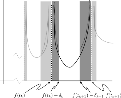
As described in Sec. 2, the limiting form of I_f(r) as r→2 will now be derived. The first step is to observe that the integral in Eq. 6 may split into two parts, one corresponding to the region where the function is clearly bounded and one corresponding to its singularities as shown in Fig. 11. Thus,

$${\int }_{f\left(t_k\right)}^{f\left(t_{k+1}\right)-{\delta }_{k+1}}{w}_f{\left(y\right)}^{2-ϵ}dy={\int }_{f\left(t_k\right)}^{f\left(t_k\right)+{\delta }_k}{w}_f{\left(y\right)}^{2-ϵ}dy+{\int }_{f\left(t_k\right)+{\delta }_k}^{f\left(t_{k+1}\right)-{\delta }_{k+1}}{w}_f{\left(y\right)}^{2-ϵ}dy={\int }_{f\left(t_k\right)}^{f\left(t_k\right)+{\delta }_k}{w}_f{\left(y\right)}^{2-ϵ}dy+B_k,$$ (A1)

where we have written B_k for the integral over the unshaded region between f(t_k)+δ_k and f(t_k+1)−δ_k+1 in Fig. 11. We observe that B_k is bounded as ϵ→0, while the integral appearing in Eq. A1 is not.

Figure 11.

An enlarged plot of a singularity of the density function w_f(y)^2−ϵ (solid curve) and Eq. 5 (dashed curves); quantities relevant for derivation of Eq. A12. As the shaded regions shrink the ratio between the dashed and solid curves approaches 1. The darker shading corresponds to the region discussed in the text.

Next, we consider the small interval of length δ_k near the singularity of w_f(f(t_k)) (shaded regions of Fig. 11). This is the singularity corresponding to the kth extrema of f(t): f(t_k); also shown is the adjacent singularity corresponding to an extrema of f(t) at t_k+1. The dashed lines in these regions represent the one over square root limiting form described in Eq. 5. By choosing δ_k small enough we may make the ratio of the solid and dashed curves arbitrarily close to 1. In other words, Eqs. 1, 5 tell us that in these shaded regions the following difference can be made as small as we like:

$$\mid w_f\left(y-{\delta }_k\right)∕\frac{a_k}{\sqrt{y-f\left(t_k\right)}}-1\mid ,$$ (A2)

where $a_k=\sqrt{2∕f^{″}\left(t_k\right)}=\sqrt{2∕\mid f^{″}\left(t_k\right)\mid }$ [assuming a minimum at f(t_k), the argument for a maximum is similar]. Moreover, if a particular choice of δ_k yields the desired accuracy, i.e., makes the difference small enough, choosing a smaller value of δ_k will produce greater accuracy. Since the number of extrema in our time-domain function f(t) is finite, we pick the minimum δ_k, call it δ, yielding the desired accuracy in all of the shaded regions [i.e., at all singular points of w_f(y)]. With this choice of δ Eq. A1 becomes

$${\int }_{f\left(t_k\right)}^{f\left(t_{k+1}\right)-\delta }{w}_f{\left(y\right)}^{2-ϵ}dy={\int }_{f\left(t_k\right)}^{f\left(t_k\right)+\delta }{w}_f{\left(y\right)}^{2-ϵ}dy+{\tilde{B}}_k,$$ (A3)

and Eq. A2 becomes

$$\mid w_f\left(y-\delta \right)∕\frac{a_k}{\sqrt{y-f\left(t_k\right)}}-1\mid <E,$$ (A4)

or

$$w_f\left(y-\delta \right)∕a_k∕\sqrt{y-f\left(t_k\right)}=1\pm E\left(y\right),$$ (A5)

where E>∣E(y)∣ may be chosen to be as small as we like by choosing small enough δ. As a result

$$w_f{\left(y-\delta \right)}^{2-ϵ}={\left(\frac{a_k}{\sqrt{y-f\left(t_k\right)}}\right)}^{2-ϵ}{\left[1\pm E\left(y\right)\right]}^{2-ϵ}={\left(\frac{a_k}{\sqrt{y-f\left(t_k\right)}}\right)}^{2-ϵ}\left[1\pm \tilde{E}\left(y\right)\right],$$ (A6)

where, once again, $\tilde{E}\left(y\right)$ may be made arbitrarily small, i.e., for every $\tilde{E}>0$ there exists some δ>0 such that $\tilde{E}>\mid \tilde{E}\left(y\right)\mid$ for all y in between f(t_k) and f(t_k)+δ.

Combining Eqs. A3, A6 now yields

$${\int }_{f\left(t_k\right)}^{f\left(t_k\right)+\delta }{w}_f{\left(y\right)}^{2-ϵ}dy+{\tilde{B}}_k={\int }_{f\left(t_k\right)}^{f\left(t_k\right)+\delta }{\left(\frac{a_k}{\sqrt{y-f\left(t_k\right)}}\right)}^{2-ϵ}\left[1\pm \tilde{E}\left(y\right)\right]dy+{\tilde{B}}_k={\int }_{f\left(t_k\right)}^{f\left(t_k\right)+\delta }{\left(\frac{a_k}{\sqrt{y-f\left(t_k\right)}}\right)}^{2-ϵ}dy\pm {\int }_{f\left(t_k\right)}^{f\left(t_k\right)+\delta }{\left(\frac{a_k}{\sqrt{y-f\left(t_k\right)}}\right)}^{2-ϵ}\tilde{E}\left(y\right)dy+\tilde{\tilde{B}}.$$ (A7)

The second integral above may be bounded by

$$\mid {\int }_{f\left(t_k\right)}^{f\left(t_k\right)+\delta }{\left(\frac{a_k}{\sqrt{y-f\left(t_k\right)}}\right)}^{2-ϵ}\tilde{E}\left(y\right)dy\mid \le {\int }_{f\left(t_k\right)}^{f\left(t_k\right)+\delta }{\left(\frac{a_k}{\sqrt{y-f\left(t_k\right)}}\right)}^{2-ϵ}\mid \tilde{E}\left(y\right)\mid dy\le {\int }_{f\left(t_k\right)}^{f\left(t_k\right)+\delta }{\left(\frac{a_k}{\sqrt{y-f\left(t_k\right)}}\right)}^{2-ϵ}\tilde{E}dy\le \tilde{E}{\int }_{f\left(t_k\right)}^{f\left(t_k\right)+\delta }{\left(\frac{a_k}{\sqrt{y-f\left(t_k\right)}}\right)}^{2-ϵ}dy.$$ (A8)

This inequality may be converted to an equality by replacing the $\tilde{E}$ factor with a smaller (positive) number. In general, this number will depend on the behavior of w_f(y) near the singular point y=f(t_k). For clarity, we denote this constant by ${\tilde{E}}_k$. With this notation, Eq. A8 becomes

$${\int }_{f\left(t_k\right)}^{f\left(t_k\right)+\delta }{\left(\frac{a_k}{\sqrt{y-f\left(t_k\right)}}\right)}^{2-ϵ}\tilde{E}\left(y\right)dy={\tilde{E}}_k{\int }_{f\left(t_k\right)}^{f\left(t_k\right)+\delta }{\left(\frac{a_k}{\sqrt{y-f\left(t_k\right)}}\right)}^{2-ϵ}dy,$$ (A9)

where $\tilde{E}\ge {\tilde{E}}_k>0$ and hence may also be made as small as we wish by reducing δ. The common integral appearing in Eqs. A7, A8 may be computed as

$${\int }_{f\left(t_k\right)}^{f\left(t_k\right)+\delta }{\left(\frac{a_k}{\sqrt{y-f\left(t_k\right)}}\right)}^{2-ϵ}dy=a_k^{2-ϵ}{\int }_{f\left(t_k\right)}^{f\left(t_k\right)+\delta }{\left(y-f\left(t_k\right)\right)}^{1-ϵ∕2}dy$$ (A10)

$$=a_k^{2-ϵ}{\phantom{\mid }\frac{{\left(y-f\left(t_k\right)\right)}^{ϵ∕2}}{ϵ∕2}\mid }_{f\left(t_k\right)}^{f\left(t_k\right)+\delta }$$

$$=a_k^{2-ϵ}\frac{{\left(f\left(t_k\right)+\delta -f\left(t_k\right)\right)}^{ϵ∕2}}{ϵ∕2}$$

$$=\frac{2a_k^2{\delta }^{ϵ∕2}}{ϵ},$$

so that Eq. A7 becomes

$${\int }_{f\left(t_k\right)}^{f\left(t_{k+1}\right)-\delta }{w}_f{\left(y\right)}^{2-ϵ}dy=\frac{2a_k^2{\delta }^{ϵ∕2}}{ϵ}\pm {\tilde{E}}_k\frac{2a_k^2{\delta }^{ϵ∕2}}{ϵ}+{\tilde{\tilde{B}}}_k$$ (A11)

$$=\frac{2a_k^2{\delta }^{ϵ∕2}}{ϵ}\left[1\pm {\tilde{E}}_k\right]+{\tilde{\tilde{B}}}_k,$$

which we sum over all minima to obtain

$$=\sum _{\begin{array}{c}k\\ f^{″}\left(t_k\right)>0\end{array}}\frac{2a_k^2{\delta }^{ϵ∕2}}{ϵ}\left[1\pm {\tilde{E}}_k\right]+{\tilde{\tilde{B}}}_k,$$ (A12)

a sum of bounded and unbounded terms, whose unbounded term is computable directly from the experimentally accessible function f(t) using $a_k=\sqrt{2∕f^{″}\left(t_k\right)}=\sqrt{2∕\mid f^{″}\left(t_k\right)\mid }$.

For the maximum we have the asymptotic term

$${\int }_{f\left(t_k\right)-\delta }^{f\left(t_k\right)}{\left(\frac{a_k}{\sqrt{f\left(t_k\right)-y}}\right)}^{2-ϵ}dy.$$ (A13)

So that the contribution to Eq. 6 from all of the maxima becomes

$${\int }_{f\left(t_k\right)-\delta }^{f\left(t_k\right)}{\left(\frac{a_k}{\sqrt{f\left(t_k\right)-y}}\right)}^{2-ϵ}dy=a_k^{2-ϵ}{\int }_{f\left(t_k\right)-\delta }^{f\left(t_k\right)}{\left(f\left(t_k\right)-y\right)}^{1-ϵ∕2}dy$$ (A14)

$$=a_k^{2-ϵ}{\phantom{\mid }\frac{{\left(f\left(t_k\right)-y\right)}^{ϵ∕2}}{ϵ∕2}\mid }_{f\left(t_k\right)-\delta }^{f\left(t_k\right)}$$

$$=a_k^{2-ϵ}\frac{{\left(f\left(t_k\right)-f\left(t_k\right)+\delta \right)}^{ϵ∕2}}{ϵ∕2}$$

$$=\frac{2a_k^2{\delta }^{ϵ∕2}}{ϵ},$$

we now have a different expression for $a_k=\sqrt{-2∕f^{″}\left(t_k\right)}=\sqrt{2∕\mid f^{″}\left(t_k\right)\mid }$.

Adding the contributions for the maxima and minima we obtain

$${\int }_{f_{\text{min}}}^{f_{\text{max}}}{w}_f{\left(y\right)}^{2-ϵ}dy=\sum _{\left\{t_k\mid f^{\prime }\left(t_k\right)=0\right\}}\frac{2a_k^2{\delta }^{ϵ∕2}}{\int }\left[1\pm {\tilde{E}}_k\right]+{\tilde{\tilde{B}}}_k$$ (A15)

$$=\sum _{\left\{t_k\mid f^{\prime }\left(t_k\right)=0\right\}}\frac{4{\delta }^{ϵ∕2}}{ϵ\mid f^{″}\left(t_k\right)\mid }\left[1\pm {\tilde{E}}_k\right]+{\tilde{\tilde{B}}}_k.$$

Cross multiplying by ϵ

$$ϵ{\int }_{f_{\text{min}}}^{f_{\text{max}}}{w}_f{\left(y\right)}^{2-ϵ}dy=\sum _{\left\{t_k\mid f^{\prime }\left(t_k\right)=0\right\}}\frac{4{\delta }^{ϵ∕2}}{\mid f^{″}\left(t_k\right)\mid }\left[1\pm {\tilde{E}}_k\right]+ϵ{\tilde{\tilde{B}}}_k,$$ (A16)

taking the logarithm of both sides and letting ϵ→0 we have

$$\underset{ϵ\to 0}{\text{lim}}\left(\text{log}\int +\text{log}\left[{\int }_{f_{\text{min}}}^{f_{\text{max}}}{w}_f{\left(y\right)}^{2-\int }dy\right]\right)=\text{log}\left[4\sum _{\left\{t_k\mid f^{\prime }\left(t_k\right)=0\right\}}\frac{1}{\mid f^{″}\left(t_k\right)\mid }\left[1\pm {\tilde{E}}_k\right]\right].$$ (A17)

Now taking the limit δ→0 so that the ${\tilde{E}}_k\to 0$ we obtain

$$\underset{\int \to 0}{\text{lim}}\left(\text{log}ϵ+\text{log}\left[{\int }_{f_{\text{min}}}^{f_{\text{max}}}{w}_f{\left(y\right)}^{2-ϵ}dy\right]\right)=\text{log}\left[4\sum _{\left\{t_k\mid f^{\prime }\left(t_k\right)=0\right\}}\frac{1}{\mid f^{″}\left(t_k\right)\mid }\right].$$ (A18)

This shows that as ϵ→0, the leading term in log∫w_f(y)^2−ϵdy always behaves like log 1∕ϵ, regardless of f(t); but the next term in the asymptotic expansion, the right-hand side of Eq. A18, does depend critically on f(t), and is the quantity we seek.

Multiplying both sides by 1∕(1−r)=1∕(1−2+ϵ)→−1 and then cancelling minus signs on both sides of the equation, we obtain

$$\underset{ϵ\to 0}{\text{lim}}\left(-\text{log}ϵ-I_f\left(2-ϵ\right)\right)=-\text{log}\left[4\sum _{\left\{t_k\mid f^{\prime }\left(t_k\right)=0\right\}}\frac{1}{\mid f^{″}\left(t_k\right)\mid }\right].$$ (A19)

For imaging applications, where offset removal and rescaling are typically performed when pixel values are assigned, we define the new quantity

$$I_{f,\infty }\equiv -\underset{ϵ\to 0}{\text{lim}}{I}_f\left(2-ϵ\right)-\text{log}4+\text{log}ϵ=\text{log}\left[\sum _{\left\{t_k\mid f^{\prime }\left(t_k\right)=0\right\}}\frac{1}{\mid f^{″}\left(t_k\right)\mid }\right].$$ (A20)

We will use this quantity to generate the images presented in Sec. 4.

References

- Hughes M. S., McCarthy J. E., Marsh J. N., Arbeit J. M., Neumann R. G., Fuhrhop R. W., Wallace K. D., Thomas T., Smith J., Agyem K., Znidersic D. R., Maurizi B. N., Baldwin S. L., Lanza G. M., and Wickline S. A., “Application of Renyi entropy to detect subtle changes in scattering architecture,” J. Acoust. Soc. Am. 125, 3141–3145 (2009). 10.1121/1.3097489 [DOI] [PMC free article] [PubMed] [Google Scholar]
- Hughes M. S., McCarthy J. E., Marsh J. N., Arbeit J. M., Neumann R. G., Fuhrhop R. W., Wallace K. D., Znidersic D. R., Maurizi B. N., Baldwin S. L., Lanza G. M., and Wickline S. A., “Properties of an entropy-based signal receiver with an application to ultrasonic molecular imaging,” J. Acoust. Soc. Am. 121, 3542–3557 (2007). 10.1121/1.2722050 [DOI] [PubMed] [Google Scholar]
- Bucy R. S. and Joseph P. D., Filtering for Stochastic Processes With Applications to Guidance (Chelsea, New York, 1987). [Google Scholar]
- Wiener N., Extrapolation, Interpolation, and Smoothing of Stationary Time Series: With Engineering Applications (MIT, Cambridge, MA, 1949). [Google Scholar]
- Grenander U. and Rosenblatt M., Statistical Analysis of Stationary Time Series (Chelsea, New York, 1984). [Google Scholar]
- Cover T. M. and Thomas J. A., Elements of Information Theory (Wiley-Interscience, New York, 1991). [Google Scholar]
- Tolman R., The Principles of Statistical Mechanics (Dover, New York, 1979). [Google Scholar]
- Press W. H., Teukolsky S. A., Vetterling W. T., and Flannery B. P., Numerical Recipes in C, 2nd ed. (Cambridge University Press, Cambridge, 1992). [Google Scholar]
- Hughes M., Marsh J., Hall C., Fuhrhop R. W., Lacy E. K., Lanza G. M., and Wickline S. A., “Acoustic characterization in whole blood and plasma of site-targeted nanoparticle ultrasound contrast agent for molecular imaging,” J. Acoust. Soc. Am. 117, 964–72 (2005). 10.1121/1.1810251 [DOI] [PubMed] [Google Scholar]
- Flacke S., Fischer S., Scott M. J., Fuhrhop R. J., Allen J. S., McLean M., Winter P., Sicard G. A., Gaffney P. J., Wickline S. A., and Lanza G. M., “Novel MRI contrast agent for molecular imaging of fibrin implications for detecting vulnerable plaques,” Circulation 104, 1280–1285 (2001). 10.1161/hc3601.094303 [DOI] [PubMed] [Google Scholar]
- Lanza G. M., Wallace K. D., Scott M. J., Cacheris W. P., Abendschein D. R., Christy D. H., Sharkey A. M., Miller J. G., Gaffney P. J., and Wickline S. A., “A novel site-targeted ultrasonic contrast agent with broad biomedical application,” Circulation 94, 3334–3340 (1996). [DOI] [PubMed] [Google Scholar]
- Arbeit J. M., Riley R. R., Huey B., Porter C., Kelloff G., Lubet R., Ward J. M., and Pinkel D., “Chemoprevention of epidermal carcinogenesis in k14-hpv16 transgenic mice,” Cancer Res. 59, 3610–3620 (1999). [PubMed] [Google Scholar]
- Arbeit J. M., Mnger K., Howley P. M., and Hanahan D., “Progressive squamous epithelial neoplasia in k14-human papillomavirus type 16 transgenic mice,” J. Virol. 68, 4358–4368 (1994). [DOI] [PMC free article] [PubMed] [Google Scholar]