Exact Tests for Hardy–Weinberg Proportions

Abstract

Exact conditional tests are often required to evaluate statistically whether a sample of diploids comes from a population with Hardy–Weinberg proportions or to confirm the accuracy of genotype assignments. This requirement is especially common when the sample includes multiple alleles and sparse data, thus rendering asymptotic methods, such as the common χ²-test, unreliable. Such an exact test can be performed using the likelihood ratio as its test statistic rather than the more commonly used probability test. Conceptual advantages in using the likelihood ratio are discussed. A substantially improved algorithm is described to permit the performance of a full-enumeration exact test on sample sizes that are too large for previous methods. An improved Monte Carlo algorithm is also proposed for samples that preclude full enumeration. These algorithms are about two orders of magnitude faster than those currently in use. Finally, methods are derived to compute the number of possible samples with a given set of allele counts, a useful quantity for evaluating the feasibility of the full enumeration procedure. Software implementing these methods, ExactoHW, is provided.

WHEN studying the genetics of a population, one of the first questions to be asked is whether the genotype frequencies fit Hardy–Weinberg (HW) expectations. They will fit HW if the population is behaving like a single randomly mating unit without intense viability selection acting on the sampled loci. In addition, testing for HW proportions is often used for quality control in genotyping, as the test is sensitive to misclassifications or undetected null alleles. Traditionally, geneticists have relied on test statistics with asymptotic χ²-distributions to test for goodness-of-fit with respect to HW proportions. However, as pointed out by several authors (Elston and Forthofer 1977; Emigh 1980; Louis and Dempster 1987; Hernandez and Weir 1989; Guo and Thompson 1992; Chakraborty and Zhong 1994; Rousset and Raymond 1995; Aoki 2003; Maiste and Weir 2004; Wigginton et al. 2005; Kang 2008; Rohlfs and Weir 2008), these asymptotic tests quickly become unreliable when samples are small or when rare alleles are involved. The latter situation is increasingly common as techniques for detecting large numbers of alleles become widely used. Moreover, loci with large numbers of alleles are intentionally selected for use in DNA identification techniques (e.g., Weir 1992). The result is often sparse-matrix data for which the asymptotic methods cannot be trusted.

A solution to this problem is to use an exact test (Levene 1949; Haldane 1954) analogous to Fisher's exact test for independence in a 2 × 2 contingency table and its generalization to rectangular tables (Freeman and Halton 1951). In this approach, one considers only potential outcomes that have the same allele frequencies as observed, thus greatly reducing the number of outcomes that must be analyzed. One then identifies all such outcomes that deviate from the HW null hypothesis by at least as much the observed sample. The total probability of this subset of outcomes, conditioned on HW and the observed allele frequencies, is then the P-value of the test. When it is not possible to enumerate all outcomes, it is still feasible to approximate the P-value by generating a large random sample of tables.

The exact HW test has been used extensively and eliminates the uncertainty inherent in the asymptotic methods (Emigh 1980; Hernandez and Weir 1989; Guo and Thompson 1992; Rousset and Raymond 1995). However, there are two difficulties with the application of this method and its interpretation, both of which are addressed in this report.

The first issue is the question of how one decides which of the potential outcomes are assigned to the subset that deviates from HW proportions by as much as or more than the observed sample. If the alternative hypothesis is specifically an excess or a dearth of homozygotes, then the tables can be ordered by Rousset and Raymond's (1995) U-score or, equivalently, by Robertson and Hill's (1984) minimum-variance estimator of the inbreeding coefficient. However, when no specific direction of deviation from HW is suspected, then there are several possible test statistics that can be used (Emigh 1980). These include the χ²-statistic, the likelihood ratio (LR), and the conditional probability itself. The last option is by far the most widely used (Elston and Forthofer 1977; Louis and Dempster 1987; Chakraborty and Zhong 1994; Weir 1996; Wigginton et al. 2005) and implemented in the GENEPOP software package (Rousset 2008). The idea of using the null-hypothesis probability as the test statistic was originally suggested in the context of rectangular contingency tables (Freeman and Halton 1951), but this idea has been criticized for its lack of discrimination between the null hypothesis and alternatives (Gibbons and Pratt 1975; Radlow and Alf 1975; Cressie and Read 1989). For example, suppose a particular sample was found to have a very low probability under the null hypothesis of HW. Such a result would usually tend to argue against the population being in HW equilibrium. However, if this particular outcome also has a very low probability under even the best-fitting alternative hypothesis, then it merely implies that a rare event has occurred regardless of whether the population is in random-mating proportions. The first part of this report compares the use of probability vs. the likelihood ratio as the test statistic in HW exact tests. Reasons for preferring the likelihood ratio are presented.

The second difficulty in performing HW exact tests is the extensive computation needed for large samples when multiple alleles are involved. In this report I present a new algorithm for carrying out these calculations. This method adapts some of the techniques originally developed for rectangular contingency tables in which each possible outcome is represented as a path through a lattice-like network (Mehta and Patel 1983). Unlike the loop-based method currently in use (Louis and Dempster 1987), the new algorithm uses recursion and can be applied to any number of alleles without modification. In addition, it improves the efficiency by about two orders of magnitude, thus allowing the full enumeration procedure to be applied to larger samples and with greater numbers of alleles.

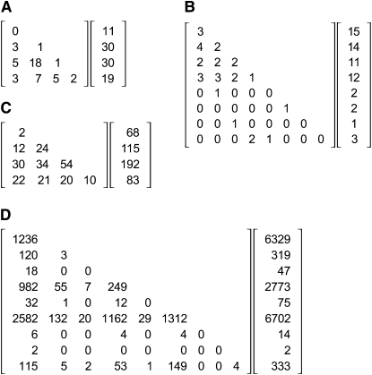
The recursion algorithm has been tested successfully on samples with as many as 20 alleles when most of those alleles are rare. However, there are still some samples for which a complete enumeration is not practical. For example, the data from the human Rh locus in Figure 1D would require examining 2 × 10⁵⁶ tables (see below). For such cases a Monte Carlo approach must be used (Guo and Thompson 1992). Several improvements to the method of independent random tables are suggested here to make that approach practical for even the largest of realistic samples, thus eliminating the need for the less-accurate Markov chain approach.

Figure 1.—

Sample data sets: examples that have been used in previous discussions of exact tests for HW proportions. For each data set, a triangular matrix of genotype counts is shown next to the vector of allele counts. (A) From Table 2, bottom row, of Louis and Dempster (1987). (B) From Figure 2 of Guo and Thompson (1992). (C) From the documentation included with the GENEPOP software package (Rousset 2008). (D) From Figure 5 of Guo and Thompson (1992).

Finally, I address the problem of determining the number of tables of genotype counts corresponding to a given set of allele counts. This number is needed for determining whether the exact test can be performed by full enumeration. Previously, this number could not be obtained except by actually carrying out the complete enumeration.

The methods described are implemented in a software package, ExactoHW, for MacOS X10.5 or later. It is available in compiled form (supporting information, File S1) or as source code for academic use on request from the author.

MATERIALS AND METHODS

All calculations were performed on a MacPro3.1 computer from Apple with two Quad-Core Intel Xeon processors running at 2.8 GHz. The operating system was MacOS X10.5. Programming for power calculations as well as the ExactoHW software was done with Apple's Xcode development system and Cocoa application programming interface. A version of GENEPOP 4.0.10 was compiled on the same equipment for use in comparisons with ExactoHW. Both GENEPOP and ExactoHW are written in dialects of C. Random permutations for the Monte Carlo procedure were obtained by the Fisher–Yates shuffle (Fisher and Yates 1943) truncated after the first n swaps in a table of 2n elements. Random numbers were generated by the multiply-with-carry method (Marsaglia 2003).

COMPARISON OF TEST STATISTICS

Formulation:

A sample of diploid genotypes at a k-allele locus can be represented by a triangular matrix such as

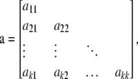where a_ij is the observed number of genotypes with alleles i and j. The number of alleles of type i is , and let n be the total sample size () and . If we assume this sample was obtained by multinomial sampling from a population in HW proportions with the observed allele frequencies , then the conditional probability of the sample given the observed allele counts is

(1)

(Levene 1949; Haldane 1954), where d is the number of homozygotes (). Equation 1 can be derived as the ratio of two multinomial probabilities. The numerator is the probability of the observed sample if the genotype frequencies fit HW expectations, and the denominator is the probability of obtaining the observed allele frequencies.

The likelihood ratio is given by

(2)

(e.g., Weir 1996, p. 106) and can also be derived as the ratio of two multinomial probabilities. The numerator is the same as for Equation 1, and the denominator is the probability of obtaining the observed outcome under the best-fitting alternative hypothesis. This best-fitting hypothesis is that of sampling from a population whose genotype frequencies are identical to those of the observed sample: . These equations can also be derived from the assumption of Poisson sampling. Interestingly, as pointed out by a reviewer, Equations 1 and 2 become interchangeable following the application of Stirling's approximation: .

Comparison of probability vs. likelihood-ratio test statistics:

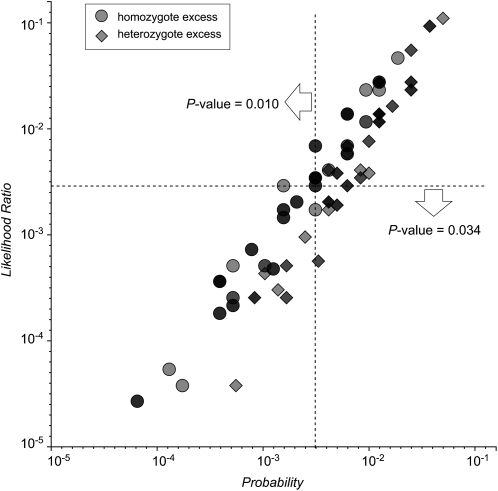
To visualize the relationship between these two types of test, consider a sample of 10 diploids containing five alleles. The allele counts are 9, 6, 3, 1, and 1. That is: . There are 139 possible samples of this kind, and their probabilities and likelihood ratios are plotted in Figure 2. It is clear that the two quantities are strongly correlated, with a nearly linear relationship when plotted on a log-log scale.

Figure 2.—

Distribution of test statistics. The likelihood ratio and probability were computed for each of the 139 possible tables with allele counts . Overlapping symbols are indicated by darker shading. Dashed lines intersect at the specific table (see text) whose P-value is being evaluated by the two exact tests. Both axes are logarithmically scaled.

One of the 139 tables,

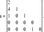is indicated by the intersection of the two dashed lines. This plot provides a graphical demonstration of the difference between the two kinds of exact test: The probability test for HW consists of summing the probabilities of all the samples that lie on or to the left of the vertical dashed line, whereas the likelihood-ratio test selects those on or below the horizontal line. The positive correlation ensures that the subsets selected by these procedures contain many of the same points. However, these subsets are not identical. They differ by the points lying in the top left and bottom right quadrants. In this case, the points in these quadrants are enough to cause a threefold difference in the computed P-values.

Visualizing the tests in this way helps to clarify why the likelihood ratio may be seen to provide a better fit to our intuitive notion of what is being tested. The points in the top left quadrant are included in the probability test because they have a slightly lower probability than the observed sample. However, it can be argued that they are not more deviant from the HW hypothesis, since their probability is relatively low even under the best-fitting alternative hypothesis. They are simply rare outcomes regardless of the true state of the population. On the other hand, those in the bottom right quadrant do seem to deviate from HW more than the observed case when compared with the best-fitting alternative. By this reasoning, the likelihood-ratio P-value of 0.034 is to be preferred over the probability-based value of 0.010 as it better reflects the strength of evidence against the HW hypothesis relative to the alternatives.

It is interesting to note that samples showing a homozygote excess relative to HW tend to lie above the diagonal in Figure 2 while many of those with a dearth of homozygotes lie below it. This tendency appears to be a general characteristic, as it was equally clear in each of several other examples plotted in this way (see Figure S1). It implies that when there is a homozygote excess, as might be caused by inbreeding or hidden subdivisions of the population, the probability-based test will tend to give a lower P-value as compared to the likelihood-ratio test. The reverse is true when there is a heterozygote excess. This trend is reflected in the power comparisons conducted in several studies (Emigh 1980; Rousset and Raymond 1995) as well as those described below.

Different alternative hypotheses:

Another useful way to compare the probability test with the likelihood-ratio test is to think of them as similar test statistics—i.e., likelihood-ratio based—but directed against different alternative hypotheses. Note that the probability test could be thought of as a likelihood-ratio test if the alternative hypothesis is that all possible conditional samples have an equal probability. That way the denominator of the likelihood ratio will be the same for all samples, and the resulting ordering of the possible samples will be identical to that produced by the probability test. However, it is not clear that any sampling procedure or realistic population characteristics would lead to all possible tables being equally likely. By contrast, multinomial sampling from a population with a fixed set of genotype frequencies is probably a good approximation to what is typically done. Therefore, this way of comparing the two tests also argues against the use of probability itself as a test statistic, as it is equivalent to performing a likelihood-ratio test against an unrealistic alternative hypothesis. It suggests that the use of LR as a test statistic may be a better choice in terms of matching a realistic set of alternative hypotheses.

Power comparisons:

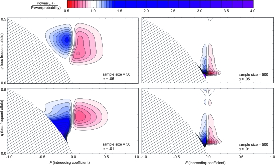
Finally, we can compare these two kinds of test in terms of their power. That is, we can compute the probability of the P-value falling below a given threshold, α, when the population deviates from HW to various extents. The contour plots in Figure 3 compare the powers of the likelihood-ratio test (numerator) with the probability test (denominator) for sample sizes of 50 and 500 and two alleles. File S2 shows other sample sizes between 10 and 600. Power comparisons of this kind have been reported previously (Emigh 1980; Hernandez and Weir 1989; Chakraborty and Zhong 1994; Rousset and Raymond 1995; Maiste and Weir 2004; Kang 2008) but not with full coverage of the parameter space. Each plot was constructed by computing the power of each test under multinomial sampling at 2687 points distributed evenly within the parameter space. The frequency, q, of the less-frequent allele can range from 0 to , and the inbreeding coefficient, F, lies between and 1.

Figure 3.—

Power comparisons. Contour plots of the ratio of the power of the exact likelihood-ratio test (numerator) and the probability test (denominator) for the case of two alleles. Sample sizes and α-levels are as shown. Each plot was constructed from a grid of 2687 points distributed uniformly throughout the parameter space of allele frequency and inbreeding coefficient. For each such point, the power was determined by generating all possible multinomial samples and summing the probabilities of those whose P-value is less than or equal to α. Mathematica (Wolfram Research) was used to draw contour curves from the computed power ratios. File S2 contains similar contour plots covering more sample sizes.

There are many areas within the parameter space where the two tests have approximately the same power, as indicated by the white spaces in Figure 3. However, there are also substantial areas where the probability test (shades of red) or the LR test (shades of blue) has significantly greater power. Even when the sample size is 500, the red and blue regions are still prominent, indicating that the two tests converge only slowly as sample size increases.

The minimum value for the ratio is ∼0.6 (Figure 3, red region), but the maximum exceeds 4.0 (purple). In other words, the decrease in relative power associated with using the LR test in the red areas is not great, but a fourfold decrease in power can result when the probability test is used for populations in the purple areas. This comparison suggest an advantage to using the LR test when there is no expectation concerning the sign of F.

The blue and purple regions in Figure 3 lie within the area where F is negative, and the red sectors occur mainly in areas where F is positive, echoing the previous observation (Emigh 1980) that the probability test can have greater power when there is an excess of homozygotes whereas the LR test's power is greater when there is a heterozygote excess. The basis for this tendency can be seen in Figure 2, where tables with a homozygote excess lie more often above the diagonal.

The red areas in Figure 3 need not be interpreted as advantageous for the probability test. On the contrary, if one accepts the arguments above, these regions of the parameter space represent situations where using the probability tests entails an increased risk of overestimating the evidence for homozygote excess. The reason is that the probability test is actually aimed at a subtly different alternative hypothesis that does not reflect realistic sampling procedures. On the other hand, the blue areas can be considered situations where the LR test has a power advantage in detecting heterozygote excess. Homozygote excess tends to be more common as it can arise from inbreeding, population subdivision, or undetected null alleles. Of course, if one type of excess is suspected initially, then the maximum power can be obtained from using a one-sided criterion such as the U-score (Rousset and Raymond 1995). A Bayesian approach can also be used to take account of prior expectations (Montoya-Delgado et al. 2001).

Contour plots similar to those in Figure 3 were also constructed to compare the LR test with χ² as the test statistic for ordering the tables (see Figure S2). The results were very similar to Figure 3, suggesting that the χ²-statistic results in an ordering that is closer to that of the probability than to the LR. This similarity might be expected, as χ² does not take explicit account of the probability of each table under the alternative hypothesis of multinomial sampling.

ALGORITHMS

Full enumeration algorithm:

A significant advance in the exact analysis of rectangular contingency tables was obtained by Mehta and Patel (1983), who found that the set of tables with fixed marginal totals could be represented by a network of nodes connected by arcs. Each pathway from the initial node to the final one corresponds to one of the tables. The total lengths of the arcs in each pathway can also be used to calculate the probability and test statistic associated with each table. This representation suggested an efficient recursion-based algorithm for enumerating the tables and computing the associated P-value.

The approach taken here is analogous, but adapted to the triangular tables of genotype data with fixed allele counts. For example, consider a sample of four diploids, each homozygous for a different allele. Thus,

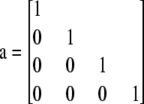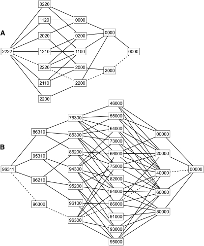
and . There are 17 possible tables with this set of allele counts. Figure 4A shows the network representation of this case. Each path from the initial node (2222) to the final one (0000) represents one of the 17 tables, and the observed table is indicated by the dashed line. The four digits identifying each node are the residual allele counts, and each column of nodes represents the genotype assignments for one of the rows of the table, starting with the bottom. These columns are referred to as levels in the contingency table literature (Mehta and Patel 1983; Agresti 1992). When tracing paths, arcs are followed only in the rightward direction. The five-allele example with 139 tables used in Figure 2 is shown in Figure 4B. Each table corresponds to one of the paths from (96311) to (00000).

Figure 4.—

Network diagrams. The tables with a given set of allele counts can be represented by the paths through a network of nodes connected by arcs. Each path begins with the leftmost node and proceeds rightward. Each node is labeled with a string of digits indicating the residual allele counts at that point. (A) Network for the case of two copies of each of four alleles. There are 17 paths from (2222) to (0000). The dashed line represents the sample in which each homozygote is observed once. (B) Network showing the 139 paths for the case of . The dashed lines specify the table that is indicated by the intersection of dashed lines in Figure 2.

To traverse the network of tables while computing the desired probabilities and test statistics, I propose an algorithm in which a pair of functions, Homozygote and Heterozygote, operate in a recursive fashion by calling themselves and each other. Each call to Homozygote corresponds to one of the nodes, whereas each arc corresponds to one or more calls to the Heterozygote function.

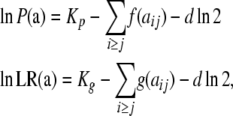
Calculation of the probability and statistics associated with each completed table is distributed through the lattice so that each new table requires minimal calculations. These calculations are greatly facilitated by noting from Equations 1 and 2 that the logs of the probability and LR can be written as

(3)

where K_p and K_g are constants that need be computed only once for the entire set of tables, and the functions, and , defined as and , respectively, are also computed only once for the integers up to the largest allele count, m_k and retrieved when needed. Note that the log of the probability is calculated initially to avoid underflow errors.

The functions Homozygote and Heterozygote take the following parameters, which must be passed by value rather than by reference, as required by the recursion process: r and c represent the current row and column, with c being unnecessary in Homozygote; f_p and g_p represent partial sums of and ; and R is an array containing the residual allele counts. Note that the quantity f_p or g_p can be thought of as the sum of the arc lengths in each path of the network diagram (Figure 4).

After the constants, K_p and K_g, and lookup tables, and , have been computed, the main calculation is initiated with a call to Homozygote with r set to k, R set to the allele counts, m₁, m₂, … , m_k, sorted in ascending order, and the remaining parameters set to zero. Presorting of the allele counts greatly increases the efficiency but does not affect the numerical outcome. The procedure below applies when there are three or more alleles. The two recursive functions are defined as follows.

Homozygote (r, f_p, g_p, R):

The first step is to compute the lower and upper bounds for a_rr given the current residual allele counts. These are

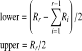with lower set to zero if the above expression is negative (Louis and Dempster 1987). Integer arithmetic is assumed where appropriate so that fractions are rounded down, thus making it unnecessary to specify whether quantities are even or odd. Now, for each value of a_rr between lower and upper, call Heterozygote with parameters in which R′ is modified from R by subtracting 2a_rr from R_r.

Heterozygote (r, c, f_p, g_p, R):

As before, we start by finding the upper and lower bounds for genotype a_rc,

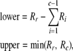with any negative value for lower replaced by zero. The next step depends on the values of r and c. If c > 2, then for each value of a_rc from lower to upper, call Heterozygote with parameters in which R′ is constructed by subtracting a_rc from each of R_r and R_c.

If c = 2 and r > 3, then for each value of a_r2 from lower to upper, let

and call Homozygote with parameters , where R′ is constructed by subtracting a_r2 from R_r and R₂ and a_r1 from R_r and R₁.

Finally, if c = 2 and r = 3, then for each value of a₃₂ from lower to upper, let

At this point, we are left with the equivalent of a two-allele case in which the allele counts are and . If , then for each value of a₁₁ from zero to we set

If , then for each value of a₂₂ from zero to we set

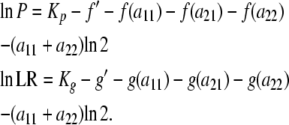
Either way, for each value we can process a completed table whose log probability and lnLR test statistic are

If the table is deemed to deviate from HW expectations at least as much as the observed table on the basis of the LR or another criterion, then the actual probability is found by taking the antilog, and the P-value is incremented by this amount.

When the initial call to Homozygote finally returns, the entire tree of tables has been traversed, all probabilities and test statistics have been computed and processed, and the exact P-values have been computed.

An enhancement to the above algorithm is the addition of the U-score test for homozygote or heterozygote excess (Rousset and Raymond 1995), which can be thought as a “one-sided” procedure for narrowing the alternative hypotheses. For the purpose of ordering the tables, the only quantity needed for each table is . By adding one more parameter to each function, this sum can be computed distributively throughout the recursion in a way similar to the other two quantities (see Equation 3). With precomputed lookup tables for (i = 1, 2), inclusion of this test statistic does not significantly increase the computation time. ExactoHW reports either or depending on whether the observed U-score is positive or negative.

To confirm that this procedure yields the same P-values as the algorithm of Louis and Dempster (1987) implemented in GENEPOP (Rousset 2008), the P-values were computed by both methods for the samples in Figure 1, A–C, and listed in Table S1. To compare the relative speeds of the algorithms, both programs were compiled from their C dialects and run on the same computer. The comparison used 4-allele samples with the same allele frequencies and sample sizes ranging from n = 500 to n = 2000. The present algorithm was found to be about two orders of magnitude faster (Table S2). The speed advantage is especially apparent in the largest sample size, where the analysis by GENEPOP required >8 hr of computation compared to <3 min for ExactoHW, even though the latter operation performed all three tests (probability, LR, and U-score) compared to probability alone.

Monte Carlo method:

Guo and Thompson (1992) suggested generating random tables of genotypes with the observed allele counts by first obtaining a random permutation of an array containing the 2n haplotypes in the observed sample. Then each pair of adjacent haplotypes in the permuted array is taken as one of the n genotypes. The probability and test statistic are then computed for each such random table, resulting in an estimate of the P-value after sufficiently many random tables have been generated. The authors concluded that this method might be useful in some cases but is not efficient enough to handle large tables owing to the necessity to compute the probability and test statistic for each table. Instead, they proposed a Markov chain alternative despite the inherent disadvantage of that method in terms of controlling the precision of the resulting P-value.

On reexamining Guo and Thompson's (1992) random sampling method, it is found that a dramatic improvement in efficiency can be obtained with a few minor modifications. The most important of these is the use of Equations 3 and the precomputed values for K_p, K_g, f, and g for finding the probability and test statistic. With this technique, the time needed for computing P and LR is small compared to that of generating the random table. An additional factor of 2 improvement can be achieved by noting that the random permutation process can be stopped after the first n elements of the randomly permuted haplotype array and then pairing haplotype i with haplotype n + i to produce each diploid genotype (see materials and methods). Finally, one can take advantage of present-day multicore computers to generate multiple random tables simultaneously.

All of these techniques are incorporated in ExactoHW. The result is that samples such as those in Figure 1, A–C, can be analyzed by the Monte Carlo method at the rate of ∼400,000 tables per second while computing all three test statistics for each. Even the much larger sample in Figure 1D is amenable to this approach, with a rate of 38,000 tables per second (Table S3). The P-values in Table S1 confirm the accuracy of this algorithm.

COUNTING TABLES

For a given data set, the choice between the full enumeration test vs. a Monte Carlo alternative depends on the number of tables needed for the full enumeration. If this number is small enough, the full enumeration is always preferable. For rectangular contingency tables, the number of possible tables with a fixed set of marginal totals has been examined by Gail and Mantel (1977) and subsequent authors (reviewed in Greselin 2004). Several exact and approximate approaches have been described with the latter being less computationally intensive. However, no similar analysis has been reported for the triangular tables associated with genotype data with fixed allele counts. The following analysis provides three alternatives to address the table-counting problem for genotypic data.

Generating function method:

The first approach is to make use of a generating function, G(x₁, x₂, … , x_k), on a set of dummy variables corresponding to the alleles. The contribution to this function from genotype ij is

Therefore, the generating function is

(4)

and the number of tables is the coefficient of in the expansion of this function. Finding this coefficient still requires computation, but with existing algorithms it can be more efficient than enumerating the entire set. In particular, the SeriesCoefficient function, which is part of the Mathematica software (Wolfram Research), works well. A Mathematica function for this task can be defined as follows:

The set of allele counts is presorted in this definition to facilitate the process, but such sorting is not needed to obtain the correct answer. With this definition, the total number of tables in the example in Figure 2 is obtained with the command count[{9, 6, 3, 1, 1}] to yield 139 tables. For the example in Figure 1A, the command count[{11, 30, 30, 19}] yields 162,365 tables; for Figure 1B count[{15, 14, 11, 12, 2, 2, 1, 3}] yields 250,552,020 tables; and for Figure 1C count[{68, 115, 192, 83}] yields 1,289,931,294 tables. These numbers are identical to those found by enumerating the entire sets.

Algorithmic approach:

The recursive algorithm described above can be modified to provide a relatively efficient count of the number of tables. Note from Figure 4 that the number of tables downstream from any node is independent of how that node was reached. Therefore, if we are interested only in the number of tables rather than their probability and test statistics, it should be necessary to traverse each node only once. When the number of tables downstream from the node has been determined, this number is placed into a hash table keyed to the identifier of the node. This identifier consists of the residuals and the node's level (see Figure 4). When this node is reached again, its downstream table count is retrieved and added to the total, eliminating the need to traverse any of the downstream nodes. This method is typically 50 times faster than complete enumeration. ExactoHW uses this algorithm to compute the needed number of tables in a separate thread to provide a quick estimate of the time needed while the full enumeration calculation is in progress.

Normal approximation:

The large sample in Figure 1D overwhelms the two exact methods described above and calls for an approximate approach. Following the strategy of Gail and Mantel (1977) for rectangular contingency tables, we start by considering a larger set of tables with fewer restrictions. Let S be the set of all possible samples of n diploids without regard to the allele counts but allowing genotypes involving any of the k alleles. The cardinality of S is known, as it represents the n-multisets of the set of genotypes. Thus

(5)

We wish to count the members of the subset S_m, which includes only those tables with allele counts m, by multiplying by the probability that a randomly selected member of S has allele counts m.

When considering a random sample from S, it is not appropriate to use the multinomial distribution, which does not assign equal probability to each distinguishable table. Instead, we make use of the one-to-one correspondence between the elements of S and the linear arrangements of n “stars” and “bars.” Each genotype count corresponds to the number of stars between adjacent bars (Feller 1968, p. 38). If a random permutation of these n + b elements is performed, then each genotype count will have expectation and probability distribution

(6)

The variance of each genotype count is found using Equation 6 to be

(7)

Also, the covariance between any two genotype counts is

(8)

Using Equations 7 and 8 plus the definition of the allele count, , we can compute the variance of each allele count

(9)

and the covariance between any pair of allele counts

(10)

With the variance–covariance matrix for m determined by Equations 9 and 10 and its mean given by , it is possible to approximate the probability of m by the multivariate normal density. To avoid singularity in the variance–covariance matrix, we can reduce the dimension to k − 1 by excluding one of the m's. This change does not affect the probability, as the sum of the allele counts is fixed. At this point, the situation becomes equivalent to Equation 3.5 of Gail and Mantel (1977), and analogous simplifications to the multivariate normal density function can be used. These simplifications arise because the m_i are equicorrelated and have a common variance. Thus

(11)

where

We can now estimate the desired number of tables from Equations 5 and 11 as .

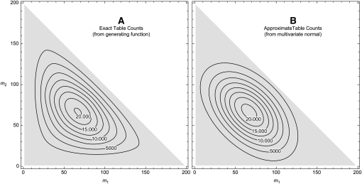
Figure 5 compares the normal approximation to the exact numbers for all possible sets of allele counts when n = 100 diploids and k = 3 alleles. The approximation is most reliable in the central region. It tends to underestimate the number of tables in the corners of the simplex and overestimate the number near the midpoint of each edge. Applying this approximation to the example in Figure 1A yields 166,195 tables, which is reasonably close to the true value of 162,365. For Figure 1B the approximation is 210,540,416 compared to the exact count of 250,552,020. For the large sample in Figure 1D, this method estimates the number of tables as 2 × 10⁵⁶, thus confirming that this sample cannot be analyzed by full enumeration.

Figure 5.—

Numbers of tables. Contour plots show the numbers of tables for each possible set of allele counts when n = 100 diploids and k = 3 alleles. (A) The exact number of tables was computed by the generating function method of Equation 4. (B) The approximate numbers of tables were found by multiplying the multivariate normal density (Equation 11) by the total cardinality (Equation 5). Note that the counts of the first two alleles are indicated while the third allele is implicit, as .

DISCUSSION

This report aims to facilitate the use of exact tests for Hardy–Weinberg proportions. Exact tests, as opposed to large-sample asymptotic approximations, are increasingly needed as data from multiallelic loci accumulate. Performing the exact tests consists of examining all—or a sampling of—the potential results having the same sample size and allele frequencies as the observed data and then finding the probability that such a sample would deviate from HW expectations by at least as much as the observed data. Although straightforward in concept, the execution can involve extensive computations. Furthermore, complications arise when one realizes that there are different ways to define the degree of deviation from HW proportions, leading to very different results.

The general question of whether probability itself should be used as a test statistic for ordering the potential outcomes of a discrete-valued experiment as opposed to using the likelihood ratio, χ², or other measures including Bayesian approaches has been examined by several authors (Gibbons and Pratt 1975; Radlow and Alf 1975; Horn 1977; Davis 1986; Cressie and Read 1989; Montoya-Delgado et al. 2001 ; Maiste and Weir 2004; Wakefield 2009), and it is unlikely that the discussion will end here. However, it is hoped that the visualization provided in Figure 2 and the accompanying discussions will at least help to clarify some of the differences and raise the possibility that the likelihood ratio may be a closer fit to what most population geneticists aim to do when testing for goodness of fit to HW proportions.

All can agree, however, that the full exact test is preferable to a Monte Carlo simulation when the former is computationally feasible. To that end, there have been two previous attempts (Aoki 2003; Maurer et al. 2007) to improve on Louis and Dempster's (1987) original algorithm for full enumeration of all tables with a given set of genotype counts. In both of those efforts, the strategy consisted of “trimming” the tree of potential tables by skipping branches that cannot contribute to the P-value or by identifying branches where the contribution can be found without traversing the entire branch. Aoki (2003) was particularly successful in finding expressions for boundaries on the minimum and maximum probabilities of tables lying downstream of a given node in the network diagram. One drawback of trimming is that only a single test can be conducted at a time, as some tables that can be skipped for one test statistic must still be evaluated for another. Both of these trimming algorithms enhanced the computational efficiency compared to the original algorithm of Louis and Dempster (1987), but they are still considerably slower than the algorithm proposed here. For example, Aoki's method was applied to the eight-allele data set in Figure 4B to perform the probability test in 625 sec, whereas ExactoHW performed all three tests (probability, likelihood ratio, and U-score) in 44 sec. This comparison is indirect, as different machines were used for the tests. However, the difference is large enough that even after considering the threefold difference in processor clock speeds used for the tests (930 MHz vs. 2.8 GHz), there is still a significant speed advantage to the present algorithm.

It might seem surprising that the algorithm proposed here and used in ExactoHW is so much more efficient than other methods despite examining many more tables compared to the trimming methods and while performing three tests rather than one. The explanation lies in the efficiency gained by distributing the calculations for the probability and test statistics throughout the recursive process. That is, each time a recursive call is made to Homozygote or Heterozygote, partial calculations are passed along so that only minimal computation is needed at each step. When this technique is combined with the precomputed tables implied by Equation 3, the computational time needed for the probability, LR, and U-score is small compared to the time needed just for generating the tables.

Despite this efficiency, it is still easy to find data sets that would require generation of too many tables to allow full enumeration by any method. The data set in Figure 1D, for example, would require ∼2 × 10⁵⁶ tables. For such cases, it is necessary to resort to a Monte Carlo simulation, for which two kinds of strategy have been proposed (Guo and Thompson 1992). The first approach is to generate a large number of independent random members of the set of tables with the same allele counts as the observed sample and use as the P-value the proportion of these tables that deviates from HW expectations as much as or more than the observed sample. Guo and Thompson (1992) proposed one method for generating such tables. Their method, with some key enhancements described above, was used in ExactoHW. An alternative method proposed by Huber et al. (2006) is optimal for very large sample sizes (n > 10⁵). The other Monte Carlo strategy makes use of a Markov chain to approximate the distribution of the test statistic (Guo and Thompson 1992; Lazzeroni and Lange 1997). This method has the disadvantage of requiring trial-and-error to determine the parameters needed to give the estimated P-value its desired precision (Guo and Thompson 1992) as opposed to the method of independent trials, which yields an estimate of the P-value whose standard error is inversely proportional to the square root of the number of trials. Fortunately, sufficiently many independent trials can be generated for any realistic sample size. For example, ExactoHW generates independent trials for the large sample in Figure 1D at the rate of 2 million tables per minute while computing the probability, LR, and U-score for each. Since this example is larger than most actual data sets, and since the number of random tables needed for an adequate estimate of the P-value is well below 1 million (Guo and Thompson 1992), it seems clear that the method is adequate for any realistic sample.

These speeds improve on existing methods of independent sampling by at least two orders of magnitude. With the Markov chain method speed is not usually an issue. However, it is worth noting that the independent trial method given here actually outpaces that of the Markov chain method when tested for a given degree of precision (see Table S3). The efficiency of the independent-sampling Monte Carlo method as implemented in ExactoHW would seem to eliminate any necessity to resort to the Markov chain approach.

One concern with any statistical procedure based on discrete data, and with the exact HW tests in particular, is that the resulting P-value takes on only discrete values (Hernandez and Weir 1989; Weir 1996). As a result, if an experimenter sets a threshold level for the P-value, α say, it may be that the actual probability of rejecting the null hypothesis when it is true is not close to α. Rohlfs and Weir (2008) derived the distribution of the P-value for the exact probability test for HW in the case of two alleles and used this information to correct the bias. This consideration can be important when it is necessary to make specific decisions on the basis of the evidence against HW proportions (Gomes et al. 1999; Salanti et al. 2005; Zou and Donner 2006). On the other hand, for most situations where no immediate decision is required, one can follow the advice of Yates (1984), who recommended for discrete data that researchers simply report the calculated P-value itself without worrying about whether it lies above or below an arbitrary cutoff point. That way, readers can interpret the exact P-value as a measure of the strength or weakness of the case against the population being in HW proportions and the genotyping being accurate and complete.

References

- Agresti, A., 1992. A survey of exact inference for contingency tables. Stat. Sci. 7 131–153. [Google Scholar]
- Aoki, S., 2003. Network algorithm for the exact test of Hardy-Weinberg proportion for multiple alleles. Biom. J. 45 471–490. [Google Scholar]
- Chakraborty, R., and Y. Zhong, 1994. Statistical power of an exact test of Hardy-Weinberg proportions of genotypic data at a multiallelic locus. Hum. Hered. 44 1–9. [DOI] [PubMed] [Google Scholar]
- Cressie, N., and T. R. C. Read, 1989. Pearson's X2 and the loglikelihood ratio statistic G2: a comparative review. Int. Stat. Rev. 57 19–43. [Google Scholar]
- Davis, L. J., 1986. Exact tests for 2 × 2 contingency tables. Am. Stat. 40 139–141. [Google Scholar]
- Elston, R. C., and R. Forthofer, 1977. Testing for Hardy-Weinberg equilibrium in small samples. Biometrics 33 536–542. [Google Scholar]
- Emigh, T. H., 1980. A comparison of tests for Hardy-Weinberg equilibrium. Biometrics 36 627–642. [PubMed] [Google Scholar]
- Feller, W., 1968. An Introduction to Probability Theory and Its Applications, Vol. 1. John Wiley & Sons, New York.
- Fisher, R. A., and F. Yates, 1943. Statistical Tables: For Biological, Agricultural and Medical Research. Oliver & Boyd, London.
- Freeman, G. H., and J. H. Halton, 1951. Note on an exact treatment of contingency, goodness of fit and other problems of significance. Biometrika 38 141–149. [PubMed] [Google Scholar]
- Gail, M., and N. Mantel, 1977. Counting the number of r × c contingency tables with fixed margins. J. Am. Stat. Assoc. 72 859–862. [Google Scholar]
- Gibbons, J. D., and J. W. Pratt, 1975. P-values: interpretation and methodology. Am. Stat. 29 20–25. [Google Scholar]
- Gomes, I., A. Collins, C. Lonjou, N. S. Thomas, J. Wilkinson et al., 1999. Hardy-Weinberg quality control. Ann. Hum. Genet. 63 535–538. [DOI] [PubMed] [Google Scholar]
- Greselin, F., 2004. Counting and enumerating frequency tables with given margins. Stat. Appl. 1 87–104. [Google Scholar]
- Guo, S. W., and E. A. Thompson, 1992. Performing the exact test of Hardy-Weinberg proportion for multiple alleles. Biometrics 48 361–372. [PubMed] [Google Scholar]
- Haldane, J., 1954. An exact test for randomness of mating. J. Genet. 52 631–635. [Google Scholar]
- Hernandez, J. L., and B. S. Weir, 1989. A disequilibrium coefficient approach to Hardy-Weinberg testing. Biometrics 45 53–70. [PubMed] [Google Scholar]
- Horn, S., 1977. Goodness-of-fit tests for discrete data: a review and an application to a health impairment scale. Biometrics 33 237–247. [PubMed] [Google Scholar]
- Huber, M., Y. Chen, I. Dinwoodie, A. Dobra and M. Nicholas, 2006. Monte Carlo algorithms for Hardy-Weinberg proportions. Biometrics 62 49–53. [DOI] [PubMed] [Google Scholar]
- Kang, S., 2008. Which exact test is more powerful in testing the Hardy–Weinberg law? Commun. Stat. Simul. Comput. 37 14–24. [Google Scholar]
- Lazzeroni, L. C., and K. Lange, 1997. Markov chains for Monte Carlo tests of genetic equilibrium in multidimensional contingency tables. Ann. Stat. 25 138–168. [Google Scholar]
- Levene, H., 1949. On a matching problem arising in genetics. Ann. Math. Stat. 20 91–94. [Google Scholar]
- Louis, E. J., and E. R. Dempster, 1987. An exact test for Hardy-Weinberg and multiple alleles. Biometrics 43 805–811. [PubMed] [Google Scholar]
- Maiste, P. J., and B. S. B. S. Weir, 2004. Optimal testing strategies for large, sparse multinomial models. Comput. Stat. Data Anal. 46 605–620. [Google Scholar]
- Marsaglia, G., 2003. Random number generators. J. Mod. Appl. Stat. Methods 2 2–13. [Google Scholar]
- Maurer, H., A. Melchinger and M. Frisch, 2007. An incomplete enumeration algorithm for an exact test of Hardy–Weinberg proportions with multiple alleles. Theor. Appl. Genet. 115 393–398. [DOI] [PubMed] [Google Scholar]
- Mehta, C. R., and N. R. Patel, 1983. A network algorithm for performing Fisher's exact test in r x c contingency tables. J. Am. Stat. Assoc. 78 427–434. [Google Scholar]
- Montoya-Delgado, L. E., T. Z. Irony, C. A. d. B. Pereira and M. R. Whittle, 2001. An unconditional exact test for the Hardy-Weinberg equilibrium law: sample-space ordering using the Bayes factor. Genetics 158 875–883. [DOI] [PMC free article] [PubMed] [Google Scholar]
- Radlow, R., and E. F. Alf, Jr., 1975. An alternate multinomial assessment of the accuracy of the chi-square test of goodness of fit. J. Am. Stat. Assoc. 70 811–813. [Google Scholar]
- Robertson, A., and W. G. Hill, 1984. Deviations from Hardy-Weinberg proportions: sampling variances and use in estimation of inbreeding coefficients. Genetics 107 703–718. [DOI] [PMC free article] [PubMed] [Google Scholar]
- Rohlfs, R. V., and B. S. Weir, 2008. Distributions of Hardy-Weinberg equilibrium test statistics. Genetics 180 1609–1616. [DOI] [PMC free article] [PubMed] [Google Scholar]
- Rousset, F., 2008. genepop'007: a complete re-implementation of the genepop software for Windows and Linux. Mol. Ecol. Res. 8 103–106. [DOI] [PubMed] [Google Scholar]
- Rousset, F., and M. Raymond, 1995. Testing heterozygote excess and deficiency. Genetics 140 1413–1419. [DOI] [PMC free article] [PubMed] [Google Scholar]
- Salanti, G., G. Amountza, E. E. Ntzani and J. P. Ioannidis, 2005. Hardy-Weinberg equilibrium in genetic association studies: an empirical evaluation of reporting, deviations, and power. Eur. J. Hum. Genet. 13 840–848. [DOI] [PubMed] [Google Scholar]
- Wakefield, J., 2009. Bayesian methods for examining Hardy-Weinberg equilibrium. Biometrics (in press). [DOI] [PMC free article] [PubMed]
- Weir, B. S., 1992. Population genetics in the forensic DNA debate. Proc. Natl. Acad. Sci. USA 89 11654–11659. [DOI] [PMC free article] [PubMed] [Google Scholar]
- Weir, B. S., 1996. Genetic Data Analysis II. Sinauer Associates, Sunderland, MA.
- Wigginton, J. E., D. J. Cutler and G. R. Abecasis, 2005. A note on exact tests of Hardy-Weinberg equilibrium. Am. J. Hum. Genet. 76 887–893. [DOI] [PMC free article] [PubMed] [Google Scholar]
- Yates, F., 1984. Test of significance for 2 × 2 contingency tables. J. R. Stat. Soc. Ser. A 147 426–463. [Google Scholar]
- Zou, G. Y., and A. Donner, 2006. The merits of testing Hardy-Weinberg equilibrium in the analysis of unmatched case-control data: a cautionary note. Ann. Hum. Genet. 70 923–933. [DOI] [PubMed] [Google Scholar]