

Abstract
Motivation: Models of regulatory networks become more difficult to construct and understand as they grow in size and complexity. Modelers naturally build large models from smaller components that each represent subsets of reactions within the larger network. To assist modelers in this process, we present model aggregation, which defines models in terms of components that are designed for the purpose of being combined.
Results: We have implemented a model editor that incorporates model aggregation, and we suggest supporting extensions to the Systems Biology Markup Language (SBML) Level 3. We illustrate aggregation with a model of the eukaryotic cell cycle ‘engine’ created from smaller pieces.
Availability: Java implementations are available in the JigCell Aggregation Connector. See http://jigcell.biol.vt.edu.
Contact: shaffer@vt.edu
1 INTRODUCTION
The physiological properties of cells are governed by macromolecular regulatory networks of great complexity (Kohn, 1999). Understanding the dynamical properties of these networks is facilitated by mathematical modeling of the biochemical reactions (Kohn, 1999; Novak and Tyson, 2003; Sible and Tyson, 2007; Tyson, 2007). These models are often implemented deterministically, as sets of non-linear differential equations, or probabilistically by Gillespie's stochastic simulation algorithm or its variants (Cao et al., 2004; Gillespie, 1977, 2001). In either case, the modeler is faced with the problem of specifying the reactions involved in a large complex network of interacting species, the rate laws describing each reaction and numerical values for the rate constants involved in each rate law. Building regulatory network models is a little like putting together a complicated jigsaw puzzle with many interlocking pieces. This complex modeling challenge is best broken down into smaller components that can later be joined together into a larger whole. The Systems Biology Markup Language (SBML, Hucka et al., 2003) was created to support the modeling of biochemical reaction networks, but the present version (Level 2) does not support the notion of model composition or aggregation. In earlier publications (Randhawa et al., 2007; 2008; Shaffer et al., 2006), we presented tools, algorithms and language extensions for SBML Level 3 for model ‘fusion’ and ‘composition’, irreversible and reversible processes (respectively) for joining existing submodels together. In this article, we present an alternative method of connecting submodels, that we call ‘aggregation’.
We illustrate the process of model aggregation with a model for the cell division cycle (Csikasz-Nagy et al., 2006). In eukaryotes, the cell cycle is controlled by a set of cyclin-dependent protein kinases (Cdks) that phosporylate-specific target proteins and thereby initiate the events of DNA replication, mitosis and cell division. As their name suggests, Cdks require association with a cyclin partner (CycA, CycB, etc.) to be active. The activity of a Cdk-Cyc dimer is controlled by interactions with a variety of regulatory proteins, including the anaphase promoting complex (APC), which, in combination with two auxiliary proteins (Cdc20 and Cdh1), degrades the cyclin component of the Cdk-Cyc dimer, and a suite of cyclin-dependent kinase inhibitors (CKI), which bind to and inhibit the Cdk-Cyc dimer. A simple model of these interactions (Fig. 1) is sufficient to reproduce (in simulation) many features of cell-cycle regulation in budding yeast (Tyson and Novak, 2001). This model shows how progress through the cell cycle can be thought of as irreversible transitions (Start and Finish) between two stable states (G1 and S-G2-M) of the regulatory system.
Fig. 1.

Reaction network for cell-cycle control in yeast. Icons are proteins, solid arrows are chemical reactions and dotted arrows represent enzymatic catalysis. The ‘CycB’ icon represents the active dimer Cdk1-CycB. SK is a starter kinase, IE is an intermediary enzyme and M is cell mass.
2 BUILDING LARGE NETWORKS
Over the last 20 years, molecular biologists have amassed a great deal of information about the genes and proteins that carry out fundamental biological processes within living cells—processes such as growth and reproduction, movement, signal reception and response, and programmed cell death. The complexity of these macromolecular regulatory networks is too great to tackle mathematically at the present time. Nonetheless, modelers have had success building dynamical models of restricted parts of the network. For example, for budding yeast cells there have been recent successful efforts to model the cell cycle (Chen et al., 2004), the pheromone signaling pathway (Kofahl and Klipp, 2004), the response to osmotic shock (Klipp et al., 2005) and the morphogenetic checkpoint (Ciliberto et al., 2003). Systems biologists need tools now to support aggregation of ‘submodels’ (such as these) into more comprehensive models of integrated regulatory networks.
Modeling languages and tools help modelers construct their models by providing a computational environment that minimizes the amount of human error during the construction step. While modelers are currently able to construct small- and medium-sized models by hand, the process is simplified by using computational tools that decrease the time taken to input a model and provide error-testing services along the way. In this article, we describe a representation and a tool that enable modelers to create large models by aggregation of submodels.
We assume that each of the submodels used in creating the larger model can be a validated model itself, with experimental data that fixes its parameters. The main motivation for creating a larger model is that there exists experimental information on the interaction of the subsystems that the submodels cannot account for. By aggregating validated submodels, we mitigate the problem of searching through large parameter spaces. The parameter estimation problem is now to ensure that the aggregated model is consistent with the original data used to validate the submodels (for which we already have good initial guesses, inherited from the submodels) and also the new data relevant to the interactions of the subsystems (which are governed by the new parameters describing how the submodels fit together).
In our experience in modeling cell-cycle regulation, we have found a modular approach to be practical for constructing large networks that encompass a broad range of experimental data and that allow many parameters to be estimated from the data in a systematic fashion (see, e.g. http://mpf.biol.vt.edu/research/budding_yeast_model/pp/). Previously submodels have been merged manually, by an informal process that can be tricky and error-prone. While trying to bring a more formal and algorithmic approach to bear on this problem, we have identified four distinct processes related to modular network construction, which we have called fusion, composition, flattening and aggregation (Shaffer et al., 2006). The first three have previously been implemented in the Fusion Wizard application (Randhawa et al., 2007), the Composition Wizard application (Randhawa et al., 2008) and the Model Flattener, all components of the JigCell system (http://jigcell.biol.vt.edu). The present article focuses on aggregation: proposing extensions for SBML Level 3 needed to describe aggregation, and presenting a prototype tool that enables aggregating (sub)models. We provide a meaningful example of aggregation using Tyson and Novak's (2001) models. This work is intended as a working template. It is compatible with the official SBML proposal for hierarchical modeling, as that proposal was derived in part from our work.
We define Model Fusion as a process that combines two or more submodels into a single unified model that contains the combined information (without redundancies) across the original collection. The identities of the original (sub)models are lost. The result of fusion is a model in the same language as the submodels [in our case standard SBML Level 2 (Hucka et al., 2003)], meaning that the same simulation and analysis tools can be applied. Beyond some size, fused models become too complex to intellectually grasp and manage as single entities. It then becomes necessary to represent large models as composites of distinct components. Thus, while model fusion is a useful tool for manipulating small- to mid-sized models, it does not seem to be a viable solution in the long run.
Model composition provides a mechanism for building models of large reaction networks. Under our definition of composition, one thinks of models not as monolithic entities, but rather as collections of smaller components (submodels) joined together. A composed model is built from two or more submodels by describing their redundancies and interactions. Composition is a reversible process, in that removing the intermodel interaction description that holds the composed model together recovers the original submodels.
While, it is appealing in short term to build larger models from pre-existing models, each developed independently for their own purposes, we believe that ultimately it will become necessary to build large models from components that have been designed for the purpose of combining them. We distinguish this approach (of models built from designed components) from model composition as described in Shaffer et al. (2006) and Randhawa et al. (2008) (where models are typically built from existing submodels, and therefore contain redundancies). We define model aggregation as a restricted form of composition that represents a collection of model elements as a single entity (a ‘module’). A module includes a specification for predetermined input and output ports. We distinguish between the terms module and submodel by defining a module to be a submodel with ports. These ports link to internal species and parameters and enable them to be accessed/referenced outside of the model in which they occur. They define the module's interface, which provides restricted access to the components within the module. The process of aggregation (connecting modules via their interface ports) allows modelers to create larger models in a controlled manner.
Model flattening converts a composed or aggregated model with some hierarchy or connections (discussed later) to one without such connections. The result of flattening is equivalent to fusing the submodels. The relationship information provided by the composition or aggregation process must be sufficient to allow flattening to take place without any further human intervention. The relationships used to describe the interactions among the submodels are lost, as the composed or aggregated model is converted into a single large (flat) model. Flattening a model allows us to use existing simulation tools, which have no support for composition or aggregation. We could think of flattening as analogous to compiling a program written in a high-level programming language (with subroutines) into the machine code ready to execute on a computer.
The XML-based SBML (Hucka et al., 2003) has become widely supported within the network modeling community. Thus, we choose to present concrete implementations for the various modeling processes through added SBML language constructs that express the necessary glue that connects submodels together. It is not necessary that our proposals be implemented in SBML, but doing so provides clear reference implementations in the same way as would expressing an algorithm in a particular programming language.
3 PRIOR WORK
There have been a number of efforts within the systems biology community to support either merging multiple SBML models or building model from components. Snoep et al. (2006) showed that it was possible to construct a large biological model in a bottom-up manner by manually linking together smaller modules. They combined a glycolysis pathway model with a glycoxylate pathway model. Bulatewicz et al. (2004) suggested an interface for model coupling and provided a number of solutions, from a brute force technique to using frameworks specifically designed to support coupling. A number of authors from domains outside systems biology find that successful composition (or model ‘reuse’) requires components that are specifically designed for the purpose (Davis and Anderson, 2004; Garlan et al., 1995; Kasputis and Ng, 2000; Malak and Paredis, 2004; Spiegel et al., 2005), and their experiences served as motivation for our approach to model aggregation.
The SemanticSBML (Liebermeister et al., 2009) tool suite facilitates merging of SBML models. It includes three tools: SBMLannotate helps users insert annotations into SBML models. SBMLcheck checks annotated models for completeness and consistency. SBMLmerge (Schulz et al., 2006) merges several annotated models. SemanticSBML is analogous to our Fusion Wizard described here in that it is intended for use with SBML Level 2 models. While it provides support for merging models based on annotations, it does not support model reuse through composition or aggregation, nor does it maintain a history of model development in the way composition and aggregation might. Process Modeling Tool (ProMoT; Ginkel et al., 2003) and E-Cell (Takahashi et al., 2003) are modeling packages that use some form of modularity. Modules in ProMoT are logical, encapsulated groupings of modeling elements that represent compartments which contain reactions, species and special signaling parts. ProMoT provides support for modularity and hierarchical modeling. It uses object-oriented models, composed from modules, and has its origins in process engineering. It provides support for importing/exporting standard SBML (Level 2). E-Cell uses an architecture where the complete model may be modularized through compartments. In this sense, modules must have some physical border and are not only logical or functional groupings but represent an object in the physical topology of the cell. Three additional reference frameworks exist that provide some form of composition, CellML (Lloyd et al., 2004), the Modelica language (Elmqvist et al., 2001) and JSim (Raymond et al., 2003). CellML includes a mechanism for composing models out of components. While this is not directly applicable to SBML, it can be used as a guide for composition within SBML and to facilitate future interoperability between CellML and SBML. The Modelica language provides for hierarchical object-oriented composition of components, while JSim is a Java-based modeling framework that provides a way to do object-oriented composition.
Proposals have been made within the SBML community (Finney, 2003; Ginkel, 2002; Schroder and Weimar, 2003) that describe the mechanics of composition (or aggregation) through additional SBML language features, as we will do. However, none of these proposals has been published in the peer-reviewed literature, nor to our knowledge have any been implemented. While some commercial tools might have more or less support for various forms of composition, we are unaware of any non-proprietary implementations for model composition (or aggregation) in this application domain, or any publications describing proprietary features in commercial applications. Composition and aggregation for pathway models remains very much an open problem.
Our work focuses on how to support aggregated models. The SBML language extensions that we propose elaborate on those originally presented in Finney (2003). Our implementation differs from Finney (2003) in a number of ways. The notion of <instance> structures that enabled model reuse using XLink (DeRose et al., 2001) to instantiate any number of models to access them has been replaced by adding a new XPointer (Grosso et al., 2006) attribute to the <model> structure. In this way, we minimize the number of additional SBML language constructs needed while still allowing for model reuse. The <link> structure also differs significantly from the one proposed by Finney (2003). Previous proposals have highlighted the need for imposing restrictions on linkages in an aggregated model without identifying these restrictions. Our implementation checks for circular linkages and incorporates the notion of direct links (Finney, 2003) connecting the external interfaces of the submodels together [in contrast with connecting entities within (sub)models to each other]. Section 6 provides an example using SBML syntax of three models.
4 MODEL AGGREGATION
Real molecular networks seem to be made up of simpler modules that carry out specific tasks (Tyson et al., 2003). By allowing modelers to substitute an aggregate for groups of reactions, and enabling aggregated modules to be connected to one another, we envision that model construction will become faster and more intuitive while holding true to the apparant structure of the organism being modeled. Modularization is defined here as the process of grouping reactions together as a single entity (a module) with a defined set of inputs and outputs (called ports). A module is not a simplification of the group of reactions (or their behavior). It is representational, and is used to aid better understanding of how parts of the model (the modules) interact with each other. Aggregation is the process of connecting modules together (by linking outputs of one module to inputs of another) in order to create a larger model (an aggregate of modules).
The fundamental difference between aggregation and composition [as we define it in Randhawa et al. (2008)] is the amount of access to model information and the initial source of these components. The basic building blocks for composition and aggregation are the same—a collection of one or more reactions. However, in composition, a component's information is not hidden from other components. A modeler can link to any variable or component within a submodel. In aggregation, model information is deliberately hidden to control complexity, and a modeler can only link to variables or components that are explicitly made visible (through ports) in a given module. Components for composition are typically pre-existing models that thus might contain redundancies between components and were not created with the intent of combining with other components. Part of the infrastructure for ‘gluing’ together submodels in composition is a mechanism for eliminating redundancies in submodels. No such mechanism exists for aggregation, because modules are designed to be connected.
A major benefit of aggregation is that the modeler does not need to know all the reactions within a module in order to use it, only its list of input and output ports. The ports must be defined so that modules can be linked together unambiguously. To this end, we require that an input port must be an entity with a fixed value within the module, for example, a rate constant or a reaction modifier that is a parameter in the module. An output port, on the other hand, must be one of the time-dependent variables in the submodel, that is, a reactant or product in any reaction within the module. By enforcing these constraints, we ensure that a consistent set of differential equations will always be produced when modules are linked together.
There is no difficulty in linking a variable X(t) in Module 1 to a parameter in Module 2, say ET=total concentration of an enzyme catalyzing a particular reaction in Module 2. In the differential equations for Module 2, the constant ET is now replaced by the variable X(t), and the differential equation defining changes in X(t) is still determined unambiguously by Module 1. But, if X(t) is linked to a time-varying species in Module 1, say A(t), then the notion of linkage is ambiguous. It might mean to identify species X and A or to add the chemical reaction X→A. In either case, such linkages are more suitably described by model composition, as defined in Randhawa et al. (2008), than by model aggregation, as defined here.
We implement aggregation with new language features for SBML. Language features previously identified for composition (Randhawa et al., 2008) are used for aggregation. We add additional language features to describe connections between modules. We refer to such constructs as ‘glue’. The language additions for SBML in Section 6 allow modelers to build aggregate models from modules. They support multiple instances of a given module. The features define the hierarchy of the modules, and represent the interactions, relationships and links between the modules. Aggregation and fusion should produce the same results, as the simulation output of the fused and aggregated forms of a model should be identical. While fusion combines submodels together in an irreversible way, aggregation references module components by defining the ‘glue’ that holds the modules together. A major difference is that in fusion, the explicit description of relationships between entities within submodels is lost. Aggregation records how models were aggregated/connected together. Model aggregation is an iterative process, as models are usually constructed in increments, with modelers switching back and forth between adding components/modules to a model and fine-tuning models through simulations. Constructing aggregated models is a bottom-up process as smaller models are first aggregated together to create larger models, which can be used to create even more complex models, as previously demonstrated in Snoep et al. (2006). An aggregated model can be created from a combination of flat and/or aggregated models. Model aggregation generates an aggregation graph that describes the relations among the various modules. Changing the connections between modules in an aggregated model results in a different aggregation graph structure. Since model aggregation is a combination of constructing modules and generating aggregation graphs, a tool for aggregation should take into consideration the iterative nature of the process.
We now illustrate generating an aggregated model by connecting modules through their ports using the JigCell Aggregation Connector. The Aggregation Connector in Figure 2 has two functions: (i) it converts (sub)models to modules by specifying their ports, and (ii) it connects modules together to create aggregated models. The user interface is divided into two parts, an aggregation window (top) which allows modelers to connect modules together graphically, and an embedded JigCell Model Builder (JCMB; Vass et al., 2006) (bottom) which displays a selected module in a spreadsheet interface.
Fig. 2.

The Aggregated Model in the JigCell Aggregation Connector.
To begin aggregation, the modeler presses the ‘Open Module(s)’ button on the top left of the application window to select SBML models from a file chooser. These models can be both submodels (without defined ports) or modules (with defined ports). We assume that the modules operate in a single compartment and that the user is responsible for formulating the modules in a consistent set of units. Modules are displayed as boxes with input and output ports in the aggregation window, while submodels are only displayed as boxes without ports until such time as the modeler defines its inputs and outputs. Each module has the following components:
A name in the middle of the box.
An optional set of input ports on the left-hand side of the box.
An optional set of output ports on the right-hand side of the box.
A gray box with a ‘+’ sign in the top left-hand corner of each box, used to load the module into the Model Builder.
To see the complete model (reactions, species, etc.) or convert a model to a module (by defining the ports), the modeler loads it into an embedded copy of the JCMB. JCMB displays the module's components in a spreadsheet interface. JCMB has been extended to enable a modeler to select which species and parameters are defined as ports. An additional column was added to the species and parameters spreadsheets, respectively. After loading two or more modules onto the aggregation window, a modeler can now link the output ports of one module to the input ports of another module to create an aggregated model. The links between modules are indicated as solid black lines in Figure 2.
Once the aggregated model is completed, it can be saved in an SBML file, flattened into a standard SBML Level 2 model, or converted into a more complex module for use in future aggregation. When converting an existing aggregate model into a new module, the Aggregation Connector performs an initial best guess for the ports. Since an output port can connect to more than one input port, all the output ports of the modules connected together in the aggregate model are made into output ports in the newly created module. Input ports can only be connected once, so only those input ports that are unconnected are exposed in the newly created module as input ports.
5 DISCUSSION
To illustrate how aggregation works, our example reproduces the approach used by Tyson and Novak when building their basic model of cell-cycle control in yeast cells (Tyson and Novak, 2001). They built their model in stages starting from a simple model and then adding new pieces until they obtained a satisfactory representation of the cell-cycle control system. The first model (which we will call Module I) deals with the interaction between the cyclin B-dependent kinase (CycB) and a CKI, as shown in Figure 3. Module II deals with the antagonistic interactions between CycB and a cyclin B-degrading factor (Cdh1), as shown in Figure 4. Module III deals the interaction between CycB and a different form of the cyclin-degrading factor (Cdc20), as shown in Figure 5. Finally, Module IV contains three additional reactions (→ SK, SK → and → M), as shown in Figure 6. M increases according to a logistic rate equation, and M is decreased by a factor of 2 each time the cell divides. Cell division is triggered when CycB drops below a certain threshold, as cyclin B is degraded by Cdc20 and Cdh1 and is best represented as an event in the model (see Tyson and Novak, 2001, for details).
Fig. 3.

Module I: interaction between the cyclin B-dependent kinase (CycB) and a CKI.
Fig. 4.

Module II: interaction between CycB and a cyclin B-degrading factor (Cdh1).
Fig. 5.

Module III: interaction between CycB and a different form of the cyclin degrading factor (Cdc20).
Fig. 6.

Module IV: additional reactions for cell mass and starter kinase.
The four steps to create the Aggregate Model are as follows.
Modules I–IV are created with predefined ports in the embedded JCMB within the Aggregation Connector. For convenience, the ports are set for each module during the construction process, but could also be set or adjusted in the Aggregation Connector once the modules have been created.
Iconic representations for Modules I–IV are loaded into the Aggregation Connector (Fig. 2).
Links between ports are created by holding down the mouse button and dragging the mouse from an output port of one module to an input port of another module.
Once all the links have been created, the model may be saved as an SBML file with additional language features.
These steps produce the Aggregate Model in Figure 2, which should then be simulated to verify that its dynamic properties represents the observed behavior of growing-dividing yeast cells in expected ways. Since our current simulators require standard SBML (Level 2) input, JigCell's simulation process will automatically ‘flatten’ the aggregated model by removing the additional constructs used to describe the aggregation. Simulating the resulting model using a freely available software package called XPPAUT (Ermentrout, 2003) produces the simulation output shown in Figure 7, which closely matches the simulation output from Tyson and Novak's model [Fig. 8 in Tyson and Novak (2001)].
Fig. 7.

Simulation of the Aggregated Model using the simulation package XPPAUT.
Fig. 8.

Aggregated model showing a link between two ports in different modules and the corresponding flattened model.
6 SBML SYNTAX
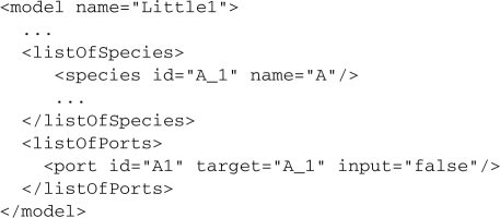
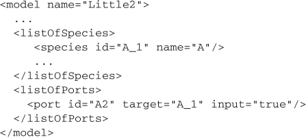
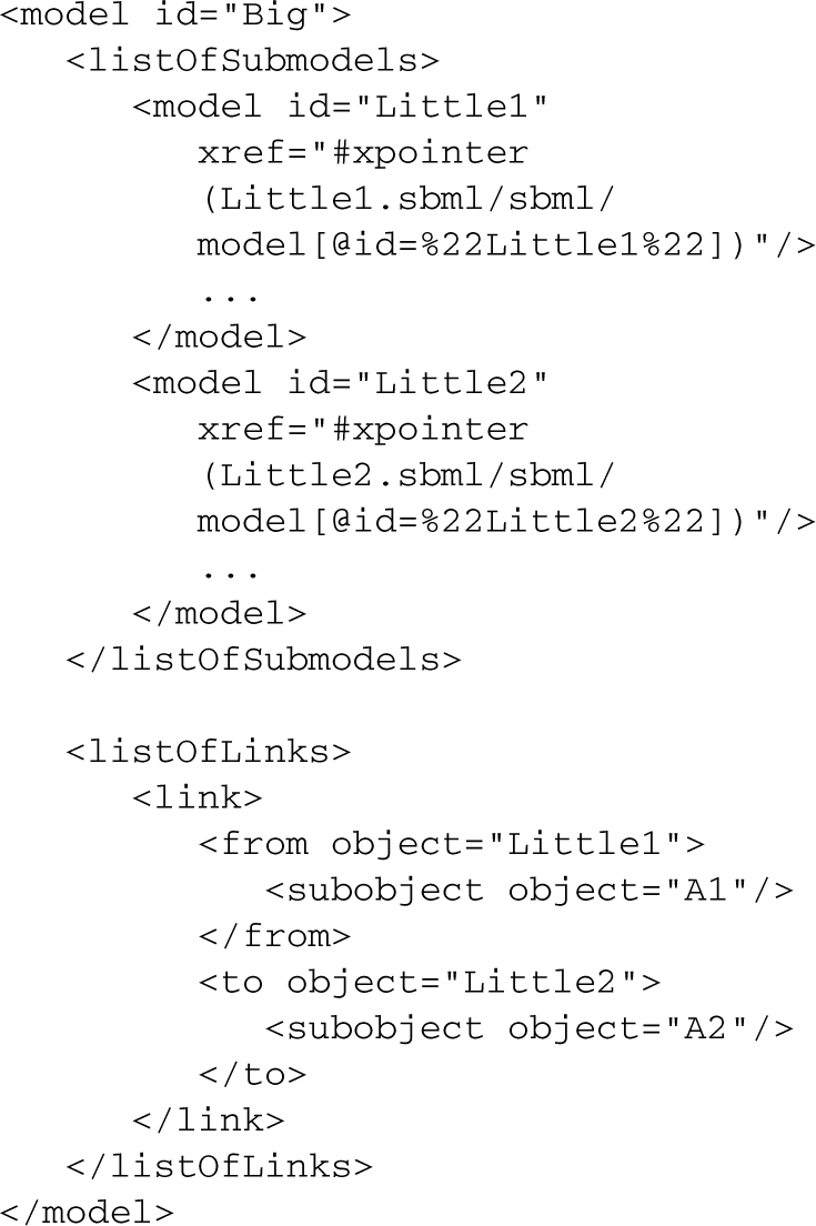
The SBML language features described below elaborate on those originally proposed in Finney (2003), by providing a defined framework with a proof of concept implementation to demonstrate the feasibility of aggregation. To illustrate the SBML language features needed to describe model aggregation, consider the example in Figure 8, which shows an aggregated model (Big) and its corresponding flattened model (Flat). Model Big contains two modules called Little1 and Little2.
To begin aggregation, we have to modify the (sub)models into modules by creating ports. The <port> (enclosed in a <listOfPorts> structure) gives a modeler access to a particular species, parameter or another port within a module for aggregation. A <port> structure is composed of three attributes: id, target and input. The id field gives a unique identifier to the port structure. The target field specifies a single species, parameter or another port by its SBML identifier. The input field specifies whether this is an input or output port. The output port structure syntax looks as follows.
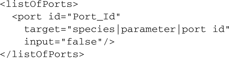
Input and output ports are distinguished from each other by their target type. <port> structures are used in conjunction with the other language constructs described below. The SBML pseudocode for the two models Little1 and Little2 indicates what needs to be added to standard SBML in order to make a module.
Once we have created the modules, we are ready to add them to the aggregated model which can contain one or more modules. A module (or submodel) is just an SBML model (enclosed within an SBML <model> structure), with its own namespace, and can itself be an aggregated model. Since there is no restriction on the number of modules a model can contain, a <model> structure is enclosed in a <listOfSubmodels> structure which contains the list of all the modules within the aggregated model.
Models can be composed from multiple instances of a particular submodel by using the XPointer framework (Grosso et al., 2006) to refer to submodels. XPointer defines a reference to another location in the current document, or an external document, using an extended pointer notation. An instance of submodel Little1 can be made within model Big to access submodel Little1 in model Big. The <model> structure contains a new attribute: an xref, which is represented using an XPointer string (Grosso et al., 2006), which is used for locating data within an XML document.
Finally, ports are connected together using the <link> structure. A <link> structure (enclosed in a <listOfLinks>) connects two ports in separate modules of an aggregated model. Linking components in aggregation can be achieved by drawing a connection between two ports in the Aggregation Connector using the mouse. A <link> is composed of two fields, <from> and <to>. The <to> field references an object (the to object) whose attribute values will be overridden by the object referenced by the <from> field (the from object). Note that a to object must refer to an input port and a from object must refer to an output port. Only those attribute values that have been declared in the from object will be overridden in the to object. This is somewhat analogous in C/C++ to treating the to object as a pointer, and the from object as its target. However, a to object can have attribute values that are retained if no overriding attribute value is declared in the from object.
We adopt a naming convention to enable modelers to uniquely identify a port within a model (or module). Our format for SBML components, such as model, species, parameter, etc., is:
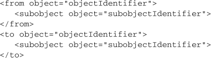
For convenience, in the description we will also represent this information using the syntax ObjectIdentifier.SubobjectIdentifier. This convention makes it possible to refer to ports with the same name in different models without having to change their names. The following example shows how the two ports (A in Little1 and A in Little2) in the aggregated model (Big) can be linked together. Information from models Little1 and Little2 is left out for simplicity and to avoid duplication. The SBML syntax below lists the modules, and contains one link between Little1.A and Little2.A.
This example shows an xref attribute where module Little1 occurs within the same SBML document. If Little1 occurred in another SBML document named temp.sbml in the current directory, the xref attribute of the <model> structure would have temp.sbml prepended to it.
In summary, the <listOfSubmodels> structure is used to define the layout of the aggregated model. Connections between the modules within the layout is made by using the <link> structures which can only connect <port> structures to each other. These three SBML language features are sufficient to define model aggregation.
7 CONCLUSIONS AND FUTURE PLANS
It is our anecdotal experience that aggregation is a faster and easier way to create models than either fusion or composition. Fusion and composition require time and effort to identify and deal with redundancies across the (sub)models. Aggregation has no such redundancies across submodels (or modules) as all submodels are customized before they are connected together. While it might take longer initially to create models for aggregation, once done it is relatively straightforward to connect them together through their ports to create larger models. We note that we are working with models we are already familiar with.
At this time we have not included support for multi-compartment models. Nor have we developed support for units and consistency checking. These features will be added in the future.
Current modeling efforts in Tyson's Group at Virginia Tech involve challenging issues in large-scale modeling. One such effort is focused on the morphogenesis checkpoint in budding yeast. Ciliberto et al. (2003) developed a model of the morphogenesis checkpoint that was ‘hooked up’ to a very primitive cell-cycle engine in budding yeast. We have successfully combined the morpho-checkpoint module with the full cell-cycle engine proposed by Chen et al. (2004) and will publish the results in the near future.
Funding: National Institutes of Health (grant R01-GM078989-01); Technology Centers for Networks and Pathways (grant U54RR022232).
Conflict of Interest: none declared.
REFERENCES
- Bulatewicz T, et al. Proceedings of the 2004 Winter Simulation Conference. NY, Piscataway, NJ: 2004. The potential coupling interface: Metadata for model coupling; pp. 183–190. Association for Computing Machinery, IEEE New York. [Google Scholar]
- Cao Y, et al. Efficient formulation of the stochastic simulation algorithm for chemically reacting systems. J. Chem. Phys. 2004;121:4059–4067. doi: 10.1063/1.1778376. [DOI] [PubMed] [Google Scholar]
- Chen K, et al. Integrative analysis of cell cycle control in budding yeast. Mol. Biol. Cell. 2004;15:3841–3862. doi: 10.1091/mbc.E03-11-0794. [DOI] [PMC free article] [PubMed] [Google Scholar]
- Ciliberto A, et al. Mathematical model of the morphogenesis checkpoint in budding yeast. J. Cell Biol. 2003;163:1243–1254. doi: 10.1083/jcb.200306139. [DOI] [PMC free article] [PubMed] [Google Scholar]
- Csikasz-Nagy A, et al. Analysis of a generic model of eukaryotic cell-cycle regulation. Biophys. J. 2006;90:4361–4379. doi: 10.1529/biophysj.106.081240. [DOI] [PMC free article] [PubMed] [Google Scholar]
- Davis P, Anderson R. Improving the composability of DoD models and simulations. J. Def. Model. Simul. 2004;1:5–17. [Google Scholar]
- DeRose S, et al. XML Linking Language (XLink) Version 1.0 W3C Recommendation. 2001 Available at http://www.w3.org/TR/xlink. [Google Scholar]
- Elmqvist H, et al. Object-oriented and hybrid modeling in modelica. Journal Européen des Systèmes Automatisés. 2001;35:1–10. [Google Scholar]
- Ermentrout B. Simulating, Analyzing, and Animating Dynamical Systems: A Guide to XPPAUT for Researchers and Students. Philadelphia: SIAM Press; 2002. Available at http://www.math.pitt.edu/∼bard/xpp/xpp.html. [Google Scholar]
- Finney A. Systems Biology Markup Language (SBML) Level 3 Proposal: model composition features. 2003 Available at http://sbml.org/images/7/73/Model-composition.pdf. [Google Scholar]
- Garlan D, et al. Architectural mismatch or why it's hard to build systems out of existing parts. International Conference on Software Engineering. 1995:179–185. Available at http://portal.acm.org/citation.cfm?doid=225014.225031. [Google Scholar]
- Gillespie D. Exact stochastic simulation of coupled chemical reactions. J. Phys. Chem. 1977;81:2340. [Google Scholar]
- Gillespie D. Approximate accelerated stochastic simulation of chemically reacting systems. J. Chem. Phys. 2001;115:1716–1733. [Google Scholar]
- Ginkel M. Systems Biology Markup Language (SBML) Level 2 Proposal: Modular SBML. 2002 Available at http://sbml.org/images/5/59/MCProposalGinkelModular.pdf. [Google Scholar]
- Ginkel M, et al. Modular modeling of cellular systems with ProMoT/Diva. Bioinformatics. 2003;19:1169–1176. doi: 10.1093/bioinformatics/btg128. [DOI] [PubMed] [Google Scholar]
- Grosso P, et al. XPointer framework. 2006 Available at http://www.w3.org/TR/xptr-framework. [Google Scholar]
- Hucka M, et al. The systems biology markup language (SBML): a medium for representation and exchange of biochemical network. Bioinformatics. 2003;19:524–531. doi: 10.1093/bioinformatics/btg015. [DOI] [PubMed] [Google Scholar]
- Kasputis S, Ng H. Proceedings of the 2000 Winter Simulation Conference. San Diego, CA, USA: Society for Computer Simulation International; 2000. Model composability: formulating a research thrust: composable simulations; pp. 1577–1584. [Google Scholar]
- Klipp E, et al. Integrative model of the response of yeast to osmotic shock. Nat. Biotechnol. 2005;23:975–982. doi: 10.1038/nbt1114. [DOI] [PubMed] [Google Scholar]
- Kofahl B, Klipp E. Modelling the dynamics of the yeast pheromone pathway. Yeast. 2004;21:831–850. doi: 10.1002/yea.1122. [DOI] [PubMed] [Google Scholar]
- Kohn K. Molecular interaction map of the mammalian cell cycle control and DNA repair systems. Mol. Biol. Cell. 1999;10:2703–2734. doi: 10.1091/mbc.10.8.2703. [DOI] [PMC free article] [PubMed] [Google Scholar]
- Liebermeister W, et al. SemanticSBML: a tool for annotating, checking, and merging of biochemical models in SBML format. Nature Precedings. 2009 Available at http://precedings.nature.com/documents/3093/version/1. [Google Scholar]
- Llyod CM, et al. CellML: its future, present and past. Prog. Biophys. Mol. Biol. 2004;85:433–450. doi: 10.1016/j.pbiomolbio.2004.01.004. [DOI] [PubMed] [Google Scholar]
- Malak R, Paredis C. Proceedings of the 2004 Winter Simulation Conference. New York, NY, Piscataway, NJ: Association for Computing Machinery, IEEE; 2004. Foundations of validating reusable behavioral models in engineering design problems; pp. 420–428. [Google Scholar]
- Novak B, Tyson JJ. Modelling the controls of the eukaryotic cell cycle. Biochem. Soc. Trans. 2003;31:1526–1529. doi: 10.1042/bst0311526. [DOI] [PubMed] [Google Scholar]
- Randhawa R, et al. Proceedings of the 2007 High Performance Computing Symposium. Piscataway, NJ, USA: IEEE Press; 2007. Fusing and composing macromolecular regulatory network models; pp. 337–344. [Google Scholar]
- Randhawa R, et al. Model composition for macromolecular regulatory networks. IEEE/ACM Trans. Comput. Biol. Bioinform. 2008;99 doi: 10.1109/TCBB.2008.64. http://doi.ieeecomputersociety.org/10.1109/TCBB.2008.64. [DOI] [PMC free article] [PubMed] [Google Scholar]
- Raymond GM, et al. JSIM: free software package for teaching phyiological modeling and research. Exp. Biol. 2003;280:102. [Google Scholar]
- Schroder D, Weimar J. Modularization of SBML. 2003 Available at http://sbml.org/images/b/bf/20041015-schroder-modularization.pdf. [Google Scholar]
- Schulz M, et al. SBMLmerge, a system for combining biochemical network models. Genome Inform. 2006;17:62–71. [PubMed] [Google Scholar]
- Shaffer CA, et al. Proceedings of the 2006 Winter Simulation Conference. Monterey, CA: 2006. The role of composition and aggregation in modeling macromolecular regulatory networks. [Google Scholar]
- Sible J, Tyson JJ. Mathematical modeling as a tool for investigating cell cycle control networks. Methods. 2007;41:238–247. doi: 10.1016/j.ymeth.2006.08.003. [DOI] [PMC free article] [PubMed] [Google Scholar]
- Snoep J, et al. Towards building the silicon cell: a modular approach. Biosystems. 2006;83:207–216. doi: 10.1016/j.biosystems.2005.07.006. [DOI] [PubMed] [Google Scholar]
- Spiegel M, et al. A case study of model context for simulation composability and reusability. Proceedings of the 2005 Winter Simulation Conference. 2005:437–444. [Google Scholar]
- Takahashi K, et al. E-Cell 2: multi-platform E-Cell simulation system. Bioinformatics. 2003;19:1727–1729. doi: 10.1093/bioinformatics/btg221. [DOI] [PubMed] [Google Scholar]
- Tyson JJ. Bringing cartoons to life. Nature. 2007;445:823. doi: 10.1038/445823a. [DOI] [PubMed] [Google Scholar]
- Tyson JJ, Novak B. Regulation of the eukaryotic cell cycle: molecular antagonism, hysteresis, and irreversible transitions. J. Theor. Biol. 2001;210:249–263. doi: 10.1006/jtbi.2001.2293. [DOI] [PubMed] [Google Scholar]
- Tyson JJ, et al. Sniffers, buzzers, toggles and blinkers: dynamics of regulatory and signaling pathways in the cell. Curr. Opin. Cell Biol. 2003;15:221–231. doi: 10.1016/s0955-0674(03)00017-6. [DOI] [PubMed] [Google Scholar]
- Vass M, et al. The JigCell Model Builder: a spreadsheet interface for creating biochemical reaction network models. IEEE/ACM Trans. Comput. Biol. Bioinform. 2006;3:155–164. doi: 10.1109/TCBB.2006.27. [DOI] [PubMed] [Google Scholar]