Use of Bayesian geostatistical prediction to estimate local variations in Schistosoma haematobium infection in western Africa

Abstract

Objective

To predict the subnational spatial variation in the number of people infected with Schistosoma haematobium in Burkina Faso, Mali and the Niger prior to national control programmes.

Methods

We used field survey data sets covering a contiguous area 2750 × 850 km and including 26 790 school-age children (5–14 years old) in 418 schools. The prevalence of high- and low-intensity infection and associated 95% credible intervals (CrIs) were predicted using Bayesian geostatistical models. The number infected was determined from the predicted prevalence and the number of school-age children in each km².

Findings

The predicted number of school-age children with a low-intensity infection was 433 268 in Burkina Faso, 872 328 in Mali and 580 286 in the Niger. The number with a high-intensity infection was 416 009, 511 845 and 254 150 in each country, respectively. The 95% CrIs were wide: e.g. the mean number of boys aged 10–14 years infected in Mali was 140 200 (95% CrI: 6200–512 100).

Conclusion

National aggregate estimates of infection mask important local variations: e.g. most S. haematobium infections in the Niger occur in the Niger River valley. High-intensity infection was strongly clustered in western and central Mali, north-eastern and north‑western Burkina Faso and the Niger River valley in the Niger. Populations in these foci will carry the bulk of the urinary schistosomiasis burden and should be prioritized for schistosomiasis control. Uncertainties in the predicted prevalence and the numbers infected should be acknowledged by control programme planners.

Introduction

An accurate estimate of the proportion of a population affected by a disease is important for prioritizing the control of that disease relative to another and for allocating resources to control or prevention programmes. Since high-quality surveillance data for developing countries is frequently lacking, calculations of the burden of a disease are often based on prevalence estimates from cross-sectional surveys, which are rarely randomized or representative of the whole population. For schistosomiasis, caused by trematodes of the genus Schistosoma, a 2003 review reported that 207 million people were infected globally and 779 million people were at risk, the majority in sub-Saharan Africa.¹ For most countries in the region, the numbers were derived from prevalence estimates contained in a 1989 report² that provided national aggregate data even though the prevalence of schistosomiasis is known to be geographically heterogeneous. In addition, previous reports have ignored uncertainties in prevalence estimates and in the size and spatial distribution of the population at risk.

Recently, empirical maps of tropical infectious diseases have been used to improve estimates of the populations infected and at risk at the continental or global level^3–5 and, increasingly, to plan and target control programmes. Advances in the production of these maps include geostatistical prediction of the prevalence of infection with Schistosoma haematobium (the aetiological agent of urinary schistosomiasis),⁶ of other parasitic infections^7–10 and of coinfections¹¹ using Bayesian methods.¹² The Bayesian approach is advantageous because the effect of covariates and spatial heterogeneity, or clustering, can be modelled simultaneously and the uncertainty of predictions can be assessed.

While the prevalence of schistosome infection has been used for planning large-scale control programmes and for estimating the disease burden, the intensity of the infection is more informative for estimating morbidity, such as urinary tract lesions and anaemia,^13–15 and plays a greater role in driving transmission than prevalence. Therefore, maps showing the average infection intensity, or the distributions of low- and high-intensity infection, might provide more effective tools than prevalence maps for estimating the disease burden and developing intervention strategies. An important statistical issue in analysing the intensity of parasitic infections is overdispersion, or aggregation, which occurs when most individuals have few parasites but a few individuals have many.¹⁶ Bayesian models have previously been used in the spatial analysis^17–19 and prediction²⁰ of the intensity of parasitic infections, due for example to Wuchereria bancrofti and Schistosoma mansoni, with overdispersion in individuals’ parasite or egg counts being modelled using the negative binomial distribution.

Burkina Faso, Mali and the Niger, three contiguous countries in the Sahelian zone of western Africa, recently conducted, coordinated, national cross-sectional, school-based, parasitological surveys.²¹ These surveys were unprecedented in their size and covered approximately 2750 km × 850 km, 26 790 school-age children and 418 schools. We aimed to use survey data to predict subnational spatial distributions of the prevalence of low- and high-intensity S. haematobium infection and to use the prediction maps to calculate the numbers of school-age children infected or at risk. We also aimed to estimate uncertainties in the predicted prevalence and the numbers infected.

Methods

Selection of schools and children

The most prevalent parasitic infection in all three study countries is S. haematobium. Programmes supported by the Schistosomiasis Control Initiative were primarily designed to control urinary schistosomiasis²¹ and our analysis includes only survey data on S. haematobium. Ethical approval for data collection was obtained from St Mary’s Hospital Research Ethics Committee in the United Kingdom, the National Public Health Research Institute’s (INRSP) scientific committee in Mali, the Ministry of Health’s ethics and scientific committees in Burkina Faso and the Ministry of Health’s ethical committee in the Niger.

Sample sizes were calculated using historical data from Mali²². It was decided to survey 87 schools in Burkina Faso, 226 in Mali and 215 in the Niger, and to include 60 children at each school. Ultimately, only 418 of the 528 schools were surveyed because remote, sparsely-populated areas had to be excluded for logistical reasons. Geographical coverage was maximized using different spatial stratification methods in the three countries. In Mali and the Niger, sample frames that contained the location of all communities were used. Spatial stratification was performed by overlaying a 1-decimal degree square grid on these countries in the ArcView version 9 (ESRI, Redlands, CA, United States of America) geographical information system. Communities were selected from the cells using simple random selection and, if they had more than one school, the study school was selected using simple random selection when the survey team arrived. In Burkina Faso, lists of schools were available for each province but were not georeferenced. The number of schools selected in each province was weighted according to the area of the province. School sampling was then done in each province using simple random selection.

The surveys were conducted from 2004–2006. The survey team determined the school’s coordinates using a global positioning system. If there were fewer than 50 boys or girls in a school, all individuals of that sex were selected because compliance was more difficult if a minority were excluded. If there were more than 50 boys or girls, 30 individuals of that sex were selected using systematic random sampling. Urine and stool samples were collected from each child and processed using standard parasitological methods. The 10-ml urine samples were passed through a filter and examined by microscope in the field. The S. haematobium egg count was recorded and entered into a Microsoft Access database (Microsoft, Redmond, WA, USA).

Predicting the prevalence of infection

Spatial prediction was based on Bayesian geostatistics.²³ Rather than modelling egg counts using the negative binomial distribution, we used a multinomial model in which the egg count was categorized as representing: (i) no infection, (ii) low-intensity infection (i.e. 1–50 eggs per 10 ml urine), or (iii) high-intensity infection (i.e. > 50 eggs per 10 ml urine). There were two reasons: (i) expediency, given that in Burkina Faso extremely high egg counts were recorded as > 1000 eggs per 10 ml urine, meaning that the upper tail of the distribution was truncated, and (ii) to facilitate future estimation of the burden of schistosomiasis because existing evidence for related morbidity is based on stratified egg counts, often using WHO definitions of low and high intensity.²⁴

It has been shown that age and sex are associated with the prevalence of urinary schistosomiasis, probably due to physiological differences in susceptibility.^25,26 Distance from a perennial inland water body is a plausible risk factor for exposure to schistosomes and subsequent infection because transmission requires contact with the aquatic habitat of intermediate host snails of the Bulinus genus. Distances were derived from an electronic perennial inland water body map obtained from the Food and Agriculture Organization of the United Nations (UN). The effect of temperature and rainfall on the distribution of Bulinus snails is reviewed in Rollinson et al.²⁷ Satellite-derived mean values for the land surface temperature and normalized difference vegetation index (a proxy for rainfall) for 1982–1998 were obtained from the National Oceanographic and Atmospheric Administration’s Advanced Very High Radiometer. The initial candidate set of variables included the individual participant variables of sex and age (categorized as 5–9 years and 10–14 years) and the school-level ecological variables of distance from a perennial inland water body, land surface temperature and normalized difference vegetation index. We tested nominal and ordinal multinomial regression models and found that a nominal model provided a better fit. Variables were selected using fixed-effects multinomial regression models in the Stata/SE 10.0 statistical package (StataCorp, College Station, TX, USA). The normalized difference vegetation index was excluded because Wald’s P was > 0.2. All remaining variables were selected for inclusion in the spatial model. This model and details of how predictions were made are presented in Box 1. The outputs of Bayesian models, including parameter estimates and spatial predictions, are termed posterior distributions. These distributions fully represent uncertainties associated with estimated values. We summarized the posterior distributions in terms of the posterior mean and 95% credible interval (CrI), within which the true value occurs with a probability of 95%.

Box 1. The Bayesian multinomial regression model with geostatistical random effects.

The spatial model was fitted in WinBUGS version 1.4 statistical software (Medical Research Council Biostatistics Unit, Cambridge, and Imperial College, London, United Kingdom). Individual raw survey data were aggregated into groups according to age, sex and location. Using three infection outcome groups (i.e. 1 = no infection, 2 = low-intensity infection, and 3 = high-intensity infection), we assumed

Y_ijk ~Multinomial(p_ijk, n_ijk), and

,

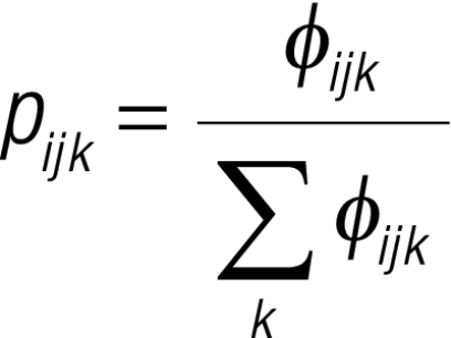where Y_ijk is the observed number of children at location i in age–sex group j and outcome group k, n_ijk is the number tested and p_ijk is the probability of infection. Here, φ_ijk can be thought of as the overall odds of being in a specific outcome group relative to not being infected. To give a reference value, φ_ij1 (i.e. for the no-infection group) was constrained to equal 1. For the other two outcome groups, we fitted the nominal regression models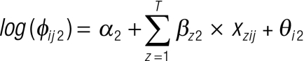, and

,

where α_k is the outcome group-specific intercept, β is a matrix of T coefficients and x is a matrix of T covariates. The θ_ik are coefficients representing location-level geostatistical random effects for the prevalence of low- and high-intensity infection. They have a multivariate normal distribution, θ_ik ~MVN(0,Σ_ik), and the variance–covariance matrices Σ_ik are defined by isotropic powered exponential spatial correlation functions

Σ_ik =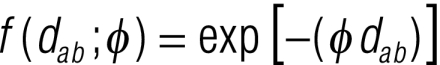

where d_ab are the distances between pairs of points a and b, and φ is the rate of decay of spatial correlation per unit distance. Noninformative priors were used for the intercepts (i.e. uniform priors with bounds −∞ and ∞) and coefficients (i.e. normal priors with a mean = 0 and a precision = 1 × 10^–4). The prior distribution of φ was also uniform, with upper and lower bounds set at 0.06 and 50. The values of the precision of the θ_ik were given noninformative gamma distributions.

A burn-in of 4000 Markov chain Monte Carlo iterations was used, followed by 1000 iterations during which values for the intercept and coefficients were stored. Diagnostic tests for convergence of the stored variables were carried out, including visual examination of history and density plots. Convergence was successfully achieved after 5000 iterations and the model was run for a further 10 000 iterations, during which the predicted prevalence at individual locations was stored for each age and sex group.

Predictions of the prevalence of low- and high-intensity infection were made at the nodes of a 0.15 × 0.15 decimal degree grid (approximately 18 km²) in WinBUGS using a spatial model and the spatial.unipred command, which used kriging to interpolate spatial random effects for low- and high-intensity infection. This assumes independence between prediction locations, as opposed to conditional predictions, and might lead to overestimation of uncertainties in the national-level estimates of numbers infected. However, conditional predictions are extremely intensive computationally and were considered as not being feasible in this study. Predicted prevalence was calculated by adding the interpolated random effect to the sum of the products of the coefficients for the fixed effects and the values of the fixed effects at each prediction location. For the individual-level fixed effects of sex and age, separate calculations were performed, in which the coefficient for the relevant age and sex group was added to the sum. The overall sum was then back-transformed from the logit scale to the prevalence scale, giving prediction surfaces that show the prevalence of low- and high-intensity infection in each age and sex group for all prediction locations.

Calculating the number infected

An electronic population surface for the study area was obtained from the Global Rural–Urban Mapping Project (GRUMP) alpha version²⁸ and imported into ArcView. In practice, GRUMP is a 30-arc second (1-km²) population raster data set that combines year 2000 census data at a subnational level with an urban-extent mask. In GRUMP, the population is redistributed using an algorithm that assumes a greater proportion is located in urban areas.²⁹

Country-specific population growth rates and the proportions of the population in given sex and age groups (i.e. 5–9 years and 10–14 years) were obtained from the UN Population Division publication World population prospects³⁰ and were used to generate population surfaces for 2005. Surfaces representing the mean and lower and upper 95% CrI limits of the predicted prevalence in each age–sex group were multiplied by the projected 2005 population surfaces using the Spatial Analyst Extension of ArcView, thereby giving the predicted number infected per km² pixel. These numbers were summed for each country.

Calculating the number at risk

By design, the multinomial model gave a predicted prevalence that was non-zero at all locations, even at those where field data indicated the absence of infection. A receiver operating characteristic analysis was conducted to determine the optimal threshold (i.e. where sensitivity = specificity) of the combined predicted prevalence (i.e. low- plus high-intensity infection prevalence) that best discriminated between schools with a zero and non-zero observed prevalence. With this approach, a predicted prevalence threshold of 5.3% gave the best discriminatory performance. A mask, created in the geographical information system to exclude areas with a combined predicted prevalence ≤ 5.3%, was overlaid on the different population surfaces for each country to calculate the numbers and proportions at risk of infection in both the school-age and total population.

Results

Predicted prevalence of infection

The total number of children aged 5–14 years included in the 2004–2006 surveys was 4808 in Burkina Faso, 14 586 in Mali and 7396 in the Niger. The raw prevalence of low-intensity infection was 10.0% (95% confidence interval, CI: 9.2–10.9) in Burkina Faso, 25.2% (95% CI: 24.5–25.9) in Mali and 10.1% (95% CI: 9.4–10.8) in the Niger. For high-intensity infection, the raw prevalence was 8.5% (95% CI: 7.7–9.3) in Burkina Faso, 11.4% (95% CI: 10.9–11.9) in Mali and 3.4% (95% CI: 3.0–3.8) in the Niger. A map of the raw prevalence of S. haematobium infection is presented in Fig. 1.

Fig. 1.

Raw prevalence of Schistosoma haematobium infection in school-age children in Burkina Faso, Mali and the Niger, 2004–2006

Image produced using ArcView version 9 (ESRI, Redlands, CA, United States of America) geographical information system.

The spatial model is presented in Table 1. It can be seen from the 95% CrI of the quadratic term for the land surface temperature that the association between this variable and the prevalence of low- or high-intensity infection was not significant. However, the distance from a perennial inland water body was significantly and negatively associated with the prevalence of both low- and high-intensity infection. In addition, the prevalence of low- and high-intensity infection was significantly higher in boys and in children aged 10–14 years than in girls or children aged 5–9 years. The rate of decay of spatial correlation was higher for low-intensity infection than high-intensity infection and the variance of the spatial random effect (i.e. the sill in geostatistical terms) was higher for high-intensity infection than low-intensity infection, which indicates a stronger propensity for spatial clustering for high-intensity infection.

Table 1. Covariates and other parameters for the Bayesian multinomial regression model used to predict^a the prevalence of low- (i.e. 1–50 eggs/10 ml urine) and high-intensity (i.e. > 50 eggs/10 ml urine) Schistosoma haematobium infection in school-age children in Burkina Faso, Mali and the Niger, 2004–2006.

Variable	Low-intensity infection Mean (95% CrI)	High-intensity infection Mean (95% CrI)
ORb for covariates
Land surface temperaturec	0.87 (0.65–1.24)	0.34 (0.12–0.57)
Land surface temperature squaredc	1.11 (0.94–1.34)	1.00 (0.78–1.30)
Distance from a PIWBc	0.36 (0.24–0.50)	0.24 (0.11–0.52)
Age, 10–14 years vs 5–9 years	1.44 (1.31–1.58)	1.45 (1.25–1.65)
Sex, female vs male	0.80 (0.74–0.86)	0.49 (0.44–0.54)
Other model parametersb
Intercept,d log odds scale	−3.04 (−3.62 to −2.51)	−4.60 (−5.13 to −3.39)
Rate of decay of the spatial correlation, φe	2.03 (1.37–2.82)	1.49 (0.75–2.29)
Variance of the spatial random effect, σ²	5.80 (4.53–7.94)	12.75 (8.92–22.27)

CrI, Bayesian credible interval; OR, odds ratio; PIWB, perennial inland water body.
^a Spatial predictions were based on a combination of the environmental covariates of land surface temperature and distance from a PIWB and the geostatistical random effect, which was described by the parameters φ and σ² (the latter represents the sill of a traditional variogram). The individual-level covariates age and sex were used to adjust the predictions for the different age–sex profiles of the survey schools.
^b The values of the ORs and parameters were derived from survey data by multiple regression.
^c The scales of the ORs were standardized for land surface temperature and distance from a PIWB by orthogonalizing the data to have a mean of 0 and standard deviation of 1.
^d The intercept represents the prevalence of infection for a male individual aged 5–9 years in a location with an average temperature and an average distance from a PIWB. Its value can be derived from the logit back-transformation and is approximately 4.5% for low-intensity infection and 1% for high-intensity infection.
^e A φ of 2.03 for low-intensity infection indicates a range of spatial correlation, equivalent to the radius of clusters, of 1.48 decimal degrees (i.e. 3/φ, approximately 170 km at the equator) after accounting for the effects of the covariates.

Separate prediction maps were produced for boys and girls and for ages 5–9 years and 10–14 years. The mean predicted prevalences of low- and high-intensity infection in boys aged 10–14 years (the highest prevalence group) are presented in Fig. 2 and Fig. 3, respectively, as illustrative examples. The maps for other age–sex groups (available from the corresponding author) showed the same spatial distribution but a lower predicted prevalence, reflecting the lower odds ratios (ORs) for infection in these groups. There were differences between the spatial distributions for low- and high-intensity infections: low-intensity infection was more widespread but the variation in prevalence was less extreme, with a predicted prevalence between 10% and 50% in most mapped areas of Burkina Faso (excluding the south-west), Mali (excluding the far south) and the Niger (excluding central regions). High-intensity infection had a more restricted spatial distribution, with defined clusters of high prevalence (> 50%) located in a mid-latitude band from western to central Mali, in northern and central Burkina Faso and in the Niger River valley in the Niger. There were large areas of low prevalence (< 5%) in southern, northern and eastern Mali, south-western Burkina Faso and most of the Niger, excluding the Niger River valley. The 95% CrI maps showed wide uncertainty in the predicted prevalence, though the prediction model was clearly able to exclude parts of each country as being at-risk areas for significant transmission of S. haematobium, as indicated by an upper 95% CrI limit for the predicted prevalence of < 5%). Fig. 4 and Fig. 5 (available at: http://www.who.int/bulletin/volumes/87/12/08-058933/en/index.html) illustrate the situation in boys 10–14 years of age; maps for other sex and age groups can be obtained from the corresponding author.

Fig. 2.

Prevalence^a of low-intensity (1–50 eggs/10 ml urine) Schistosoma haematobium infection in boys aged 10–14 years in Burkina Faso, Mali and the Niger^b in 2004–2006, as predicted using a Bayesian geostatistical multinomial regression model

^a The values presented are the posterior means obtained from the Bayesian geostatistical multinomial regression model and represent the most likely prevalence values.

^b No predictions were made for the white areas on the map.

Image produced using ArcView version 9 (ESRI, Redlands, CA, United States of America) geographical information system.

Fig. 3.

Prevalence^a of high-intensity (> 50 eggs/10 ml urine) Schistosoma haematobium infection in boys aged 10–14 years in Burkina Faso, Mali and the Niger^b in 2004–2006, as predicted using a Bayesian geostatistical multinomial regression model

^a The values presented are the posterior means obtained from the Bayesian geostatistical multinomial regression model and represent the most likely prevalence values.

^b No predictions were made for the white areas on the map.

Image produced using ArcView version 9 (ESRI, Redlands, CA, United States of America) geographical information system.

Fig. 4.

Map showing lower value for the Bayesian 95% CrI for the predicted prevalence of high-intensity (> 50 eggs/10 ml urine) Schistosoma haematobium infection in boys aged 10–14 years in Burkina Faso, Mali and the Niger^a in 2004–2006, as derived using a Bayesian geostatistical multinomial regression model

CrI, Bayesian credible interval.

^a No predictions were made for the white areas on the map.

Image produced using ArcView version 9 (ESRI, Redlands, CA, United States of America) geographical information system.

Fig. 5.

Map showing upper value for the Bayesian 95% CrI for the predicted prevalence of high-intensity (> 50 eggs/10 ml urine) Schistosoma haematobium infection in boys aged 10–14 years in Burkina Faso, Mali and the Niger^a in 2004–2006, as derived using a Bayesian geostatistical multinomial regression model

CrI, Bayesian credible interval.

^a No predictions were made for the white areas on the map.

Image produced using ArcView version 9 (ESRI, Redlands, CA, United States of America) geographical information system.

Number infected and at risk

The mean numbers of school-age children with low- and high-intensity infection in the three countries and their associated 95% CrIs are presented in Table 2. The estimated number of school-age children with low-intensity infection was 433 268 in Burkina Faso, 872 328 in Mali and 580 286 in the Niger and the number with high-intensity infection was 416 009 in Burkina Faso, 511 845 in Mali and 254 150 in the Niger. The 95% CrIs for the number infected in each age–sex group were very wide: e.g. the mean number of boys aged 10–14 years infected in Mali was 140 200 (95% CrI: 6200–512 100). Maps of the estimated number of boys aged 10–14 years with low- and high-intensity infection (Fig. 6 and Fig. 7, respectively) showed considerable within-country variation in the burden of schistosomiasis. This was also apparent for boys and girls of both age groups. As was observed with the predicted prevalence, the spatial patterns were identical for each age–sex group, though the proportion infected was uniformly lower for girls and younger boys (maps available from the corresponding author).

Table 2. Number of school-age children with low- or high-intensity Schistosoma haematobium infection in Burkina Faso, Mali and the Niger in 2005, as estimated using a Bayesian geostatistical model based on survey data from 2004–2006.

Age–sex group	Burkina Faso			Mali			the Niger
	Estimated population, in thousands	No. infected, in thousands Meana (95% CrI)		Estimated population, in thousands	No. infected, in thousands Meana (95% CrI)		Estimated population, in thousands	No. infected, in thousands Meana (95% CrI)
High-intensity infection
Boys 5–9 years	1011.0	123.9 (1.4–603.5)		1063	150.6 (6.6–567.7)		1119.9	79.3 (1.6–342.6)
Boys 10–14 years	867.2	124.0 (1.5–563.0)		896.5	140.2 (6.2–512.2)		905.9	70.8 (1.4–303.1)
Girls 5–9 years	976.8	83.5 (0.8–463.0)		1057.2	114.3 (4.1–462.2)		1065.9	55.0 (1.0–257.7)
Girls 10–14 years	840.9	84.6 (0.9–441.9)		895.3	106.8 (3.9–421.2)		860.3	49.1 (0.9–226.1)
Low-intensity infection
Boys 5–9 years	1011.0	112.0 (2.3–528.2)		1063	226.9 (18.4–687.8)		1119.9	157.4 (6.0–543.9)
Boys 10–14 years	867.2	115.9 (2.5–508.3)		896.5	218.2 (19.0–619.8)		905.9	146.2 (5.6–486.3)
Girls 5–9 years	976.8	100.3 (2.3–481.3)		1057.2	216.6 (18.5–659.9)		1065.9	143.4 (7.2–485.7)
Girls 10–14 years	840.9	105.1 (2.5–468.1)		895.3	210.7 (19.6–599.5)		860.3	133.2 (6.8–434.2)

CrI, Bayesian credible interval.
^a The mean of the posterior distribution of Bayesian estimates.

Fig. 6.

Boys aged 10–14 years with low-intensity (1–50 eggs/10 ml urine) Schistosoma haematobium infection per square kilometre in Burkina Faso, Mali and the Niger^a in 2005, as estimated using posterior means predicted by a Bayesian geostatistical multinomial regression model

^a No estimates were made for the white areas on the map.

Image produced using ArcView version 9 (ESRI, Redlands, CA, United States of America) geographical information system.

Fig. 7.

Boys aged 10–14 years with high-intensity (> 50 eggs/10 ml urine) Schistosoma haematobium infections per square kilometre in Burkina Faso, Mali and the Niger^a in 2005, as estimated using posterior means predicted by a Bayesian geostatistical multinomial regression model

^a No estimates were made for the white areas on the map.

Image produced using ArcView version 9 (ESRI, Redlands, CA, United States of America) geographical information system.

We estimated that 3.5 million, 3.4 million and 2.8 million school-age children and a total of 12.5 million (94.5% of the total population), 11.8 million (87.6% of the total) and 9.9 million (70.3% of the total) individuals of all ages were at risk of urinary schistosomiasis in Burkina Faso, Mali and the Niger, respectively. The maps (available from the corresponding author) show that there were parts of each country where people were not at risk and that could be excluded from active surveillance or nationally coordinated schistosomiasis control.

Discussion

We used robust, contemporary statistical methods in a novel application to predict the spatial distribution of S. haematobium infection. This resulted in estimates of local heterogeneity in high- and low-intensity parasitic infection that could be used in control programme planning. In 2003, Steinmann et al.¹ estimated the number of people infected with Schistosoma spp. was 7.8 million in Burkina Faso, 7.8 million in Mali and 3.2 million in the Niger by using prevalence estimates of 60.0%, 60.0% and 26.7% and assuming that the at-risk population was 100% of the estimated population, namely 13.0 million, 13.0 million and 12.0 million in the three countries, respectively. If we assume, as Steinmann et al. did, that the prevalence is the same for all age groups (which overestimates the prevalence since it is usually highest in school-age children),³¹ our estimates would be 3.0 million (23.0% of the total) in Burkina Faso, 4.8 million (35.4% of the total) in Mali and 3.0 million (21.1% of the total) in the Niger. Clearly, the previously reported number infected was considerably overestimated for Burkina Faso and Mali. In addition, the number at risk was overestimated for all three countries. We have confidence in our conclusions because our data were recent, extensive, randomized and representative. Although our calculations excluded S. mansoni infection, which Steinmann et al. included, its prevalence in our surveys was very low in Burkina Faso and the Niger, at 0.5% and 0.3%, respectively, and moderately low in Mali, at 6.7%. More importantly, Steinmann et al.’s figures overlooked important heterogeneities in the spatial distribution of people infected or at risk of schistosomiasis, which our maps capture.

The uncertainties in the numbers infected with S. haematobium captured by our model were wide despite the large sample size and the geographical coverage of the data. It might be suggested that the large uncertainties shown in our prediction maps limit their utility for decision-making. However, since tools for representing uncertainty in spatial predictions now exist and there is still a need for disease maps in planning control programmes, it is beneficial to acknowledge such uncertainties when interpreting maps for disease control. Moreover, we did not include uncertainties in the projected population or those due to population migration between areas, which are considerable in these three countries. In addition, GRUMP can produce national population totals that do not match UN totals. In 2000, GRUMP population estimates for both Mali and the Niger differed from UN estimates by more than 5%,²⁸ contributing to additional uncertainty in our updated 2005 population estimates. We also assumed that population growth was even across different regions and age groups. The limitations of the ancillary data used in GRUMP calculations have been noted elsewhere,²⁹ but currently it is impossible to quantify the resulting inaccuracies.

Our surveys were spatially stratified, which ensured equal geographical coverage of areas of both high and low population density and made the precision of predicted prevalence estimates more even across the study area. However, less densely populated areas were more strongly represented than they would have been with a nonstratified approach. Because prevalence is likely to differ between low- and high-density areas, sample weighting is necessary to ensure accurate national prevalence estimates; our map calculations are essentially a sample-weighting approach. This is evident from the difference between raw prevalence estimates for low- and high-intensity infections combined, which were 18.5% for Burkina Faso, 36.6% for Mali and 13.5% for the Niger, and map-derived estimates, which were 23.0%, 35.4% and 21.1% in the three countries, respectively. The most striking difference was for the Niger. This arose because the prevalence was highest in the Niger River valley, which has the highest population density, and in the survey this area was underrepresented, from a population perspective, relative to low-density areas.

The different spatial distributions for low- and high-intensity infection are in agreement with Guyatt et al.,¹⁶ who demonstrated that the relationship between overall prevalence and the prevalence of high-intensity infection varied geographically across Africa. While low-intensity infection was more widespread, it exhibited less spatial variability than high-intensity infection, which aggregated more into clusters.¹⁶ Future control programmes will have the greatest impact if they focus on high-intensity infection clusters.

The maps presented in this report are currently being used by national programme managers as objective decision-support tools for geographically targeting existing resources more efficiently to high-risk communities. They have several other uses. First, national programme managers can use them to argue for resources from governments or international donors, particularly after funding from the Schistosomiasis Control Initiative ends. Second, the maps can be used to formulate and compare different disease control strategies by determining the likely impact on transmission and morbidity. And lastly, they can be used for advocacy and empowerment at the subnational level: local resource needs and priorities for schistosomiasis control, which are often subsumed in aggregate national data, can be presented to national programme managers and government officials. We encourage national programme managers in other countries, and those focussing on other diseases, to conduct spatially stratified disease surveys and undertake mapping of subnational disease distributions to provide evidence for more efficient targeting of resources. ■

References

- 1.Steinmann P, Keiser J, Bos R, Tanner M, Utzinger J. Schistosomiasis and water resources development: systematic review, meta-analysis, and estimates of people at risk. Lancet Infect Dis. 2006;6:411–25. doi: 10.1016/S1473-3099(06)70521-7. [DOI] [PubMed] [Google Scholar]
- 2.Utroska JA, Chen MG, Dixon H, Yoon S, Helling-Borda M, Hogerzeil HV, et al. An estimate of global needs for praziquantel within schistosomiasis control programmes Geneva: World Health Organization; 1989. [Google Scholar]
- 3.Brooker S, Clements AC, Bundy DA. Global epidemiology, ecology and control of soil-transmitted helminth infections. Adv Parasitol. 2006;62:221–61. doi: 10.1016/S0065-308X(05)62007-6. [DOI] [PMC free article] [PubMed] [Google Scholar]
- 4.Guerra CA, Snow RW, Hay SI. Mapping the global extent of malaria in 2005. Trends Parasitol. 2006;22:353–8. doi: 10.1016/j.pt.2006.06.006. [DOI] [PMC free article] [PubMed] [Google Scholar]
- 5.Hay SI, Guerra CA, Tatem AJ, Noor AM, Snow RW. The global distribution and population at risk of malaria: past, present, and future. Lancet Infect Dis. 2004;4:327–36. doi: 10.1016/S1473-3099(04)01043-6. [DOI] [PMC free article] [PubMed] [Google Scholar]
- 6.Clements AC, Lwambo NJ, Blair L, Nyandindi U, Kaatano G, Kinung’hi S, et al. Bayesian spatial analysis and disease mapping: tools to enhance planning and implementation of a schistosomiasis control programme in Tanzania. Trop Med Int Health. 2006;11:490–503. doi: 10.1111/j.1365-3156.2006.01594.x. [DOI] [PMC free article] [PubMed] [Google Scholar]
- 7.Gemperli A, Sogoba N, Fondjo E, Mabaso M, Bagayoko M, Briet OJ, et al. Mapping malaria transmission in West and Central Africa. Trop Med Int Health. 2006;11:1032–46. doi: 10.1111/j.1365-3156.2006.01640.x. [DOI] [PubMed] [Google Scholar]
- 8.Gemperli A, Vounatsou P, Kleinschmidt I, Bagayoko M, Lengeler C, Smith T. Spatial patterns of infant mortality in Mali: the effect of malaria endemicity. Am J Epidemiol. 2004;159:64–72. doi: 10.1093/aje/kwh001. [DOI] [PubMed] [Google Scholar]
- 9.Raso G, Matthys B, N’Goran EK, Tanner M, Vounatsou P, Utzinger J. Spatial risk prediction and mapping of Schistosoma mansoni infections among schoolchildren living in western Cote d’Ivoire. Parasitology. 2005;131:97–108. doi: 10.1017/S0031182005007432. [DOI] [PubMed] [Google Scholar]
- 10.Raso G, Vounatsou P, Gosoniu L, Tanner M, N’Goran EK, Utzinger J. Risk factors and spatial patterns of hookworm infection among schoolchildren in a rural area of western Cote d’Ivoire. Int J Parasitol. 2006;36:201–10. doi: 10.1016/j.ijpara.2005.09.003. [DOI] [PubMed] [Google Scholar]
- 11.Raso G, Vounatsou P, Singer BH, N’Goran EK, Tanner M, Utzinger J. An integrated approach for risk profiling and spatial prediction of Schistosoma mansoni-hookworm coinfection. Proc Natl Acad Sci USA. 2006;103:6934–9. doi: 10.1073/pnas.0601559103. [DOI] [PMC free article] [PubMed] [Google Scholar]
- 12.Diggle P, Moyeed R, Rowlingson B, Thompson M. Childhood malaria in the Gambia: a case-study in model-based geostatistics. Appl Stat. 2002;51:493–506. [Google Scholar]
- 13.Vester U, Kardorff R, Traore M, Traore HA, Fongoro S, Juchem C, et al. Urinary tract morbidity due to Schistosoma haematobium infection in Mali. Kidney Int. 1997;52:478–81. doi: 10.1038/ki.1997.356. [DOI] [PubMed] [Google Scholar]
- 14.Abdel-Wahab MF, Esmat G, Ramzy I, Fouad R, Abdel-Rahman M, Yosery A, et al. Schistosoma haematobium infection in Egyptian schoolchildren: demonstration of both hepatic and urinary tract morbidity by ultrasonography. Trans R Soc Trop Med Hyg. 1992;86:406–9. doi: 10.1016/0035-9203(92)90241-4. [DOI] [PubMed] [Google Scholar]
- 15.Warren KS, Mahmoud AA, Muruka JF, Whittaker LR, Ouma JH, Arap Siongok TK. Schistosomiasis haematobia in coast province Kenya. Relationship between egg output and morbidity. Am J Trop Med Hyg. 1979;28:864–70. [PubMed] [Google Scholar]
- 16.Guyatt HL, Smith T, Gryseels B, Lengeler C, Mshinda H, Siziya S, et al. Aggregation in schistosomiasis: comparison of the relationships between prevalence and intensity in different endemic areas. Parasitology. 1994;109:45–55. doi: 10.1017/S0031182000077751. [DOI] [PubMed] [Google Scholar]
- 17.Alexander N, Moyeed R, Stander J. Spatial modelling of individual-level parasite counts using the negative binomial distribution. Biostatistics. 2000;1:453–63. doi: 10.1093/biostatistics/1.4.453. [DOI] [PubMed] [Google Scholar]
- 18.Alexander ND, Moyeed RA, Hyun PJ, Dimber ZB, Bockarie MJ, Stander J, et al. Spatial variation of Anopheles-transmitted Wuchereria bancrofti and Plasmodium falciparum infection densities in Papua New Guinea. Filaria J. 2003;2:14. doi: 10.1186/1475-2883-2-14. [DOI] [PMC free article] [PubMed] [Google Scholar]
- 19.Brooker S, Alexander N, Geiger S, Moyeed RA, Stander J, Fleming F, et al. Contrasting patterns in the small-scale heterogeneity of human helminth infections in urban and rural environments in Brazil. Int J Parasitol. 2006;36:1143–51. doi: 10.1016/j.ijpara.2006.05.009. [DOI] [PMC free article] [PubMed] [Google Scholar]
- 20.Clements AC, Moyeed R, Brooker S. Bayesian geostatistical prediction of the intensity of infection with Schistosoma mansoni in East Africa. Parasitology. 2006;133:711–9. doi: 10.1017/S0031182006001181. [DOI] [PMC free article] [PubMed] [Google Scholar]
- 21.Garba A, Toure S, Dembele R, Bosque-Oliva E, Fenwick A. Implementation of national schistosomiasis control programmes in West Africa. Trends Parasitol. 2006;22:322–6. doi: 10.1016/j.pt.2006.04.007. [DOI] [PubMed] [Google Scholar]
- 22.Gryseels B. Mission d’Evaluation du report, Lutte contre la schistosomiasis au Mali Eschborn: Gesellschaft für Technische Zusammenarbeit; 1989.
- 23.Diggle P, Tawn J, Moyeed R. Model-based geostatistics. Appl Stat. 1998;47:299–350. [Google Scholar]
- 24.Coordinated use of anthelminthic drugs in control interventions: a manual for health professionals and programme managers Geneva: World Health Organization; 2006. [Google Scholar]
- 25.Fulford AJ, Webster M, Ouma JH, Kimani G, Dunne DW. Puberty and age-related changes in susceptibility to schistosome infection. Parasitol Today. 1998;14:23–6. doi: 10.1016/S0169-4758(97)01168-X. [DOI] [PubMed] [Google Scholar]
- 26.Feldmeier H, Poggensee G, Krantz I. Puberty and age-intensity profiles in schistosome infections: another hypothesis. Parasitol Today. 1998;14:435. doi: 10.1016/S0169-4758(98)01313-1. [DOI] [PubMed] [Google Scholar]
- 27.Rollinson D, Stothard JR, Southgate VR. Interactions between intermediate snail hosts of the genus Bulinus and schistosomes of the Schistosoma haematobium group. Parasitology. 2001;123(Suppl):S245–60. doi: 10.1017/S0031182001008046. [DOI] [PubMed] [Google Scholar]
- 28.Global Rural–Urban Mapping Project (GRUMP) [Alpha version]. Palisades, NY: Socioeconomic Data and Applications Center, Columbia University. Available from: http://sedac.ciesin.columbia.edu/gpw [accessed on 19 June 2009].
- 29.Balk DL, Deichmann U, Yetman G, Pozzi F, Hay SI, Nelson A. Determining global population distribution: methods, applications and data. Adv Parasitol. 2006;62:119–56. doi: 10.1016/S0065-308X(05)62004-0. [DOI] [PMC free article] [PubMed] [Google Scholar]
- 30.United Nations. World population prospects: the 2006 revision New York, NY: United Nations, Department of Economic and Social Affairs, Population Division; 2007. Available from: http://www.un.org/esa/population/publications/wpp2006/wpp2006.htm [accessed on 19 June 2009].
- 31.Brooker S, Donnelly CA, Guyatt HL. Estimating the number of helminthic infections in the Republic of Cameroon from data on infection prevalence in schoolchildren. Bull World Health Organ. 2000;78:1456–65. [PMC free article] [PubMed] [Google Scholar]