Implementation of a Serial Replica Exchange Method in a Physics-Based United-Residue (UNRES) Force Field

Abstract

The kinetic-trapping problem in simulating protein folding can be overcome by using a Replica Exchange Method (REM). However, in implementing REM in molecular dynamics simulations, synchronization between processors on parallel computers is required, and communication between processors limits its ability to sample conformational space in a complex system efficiently. To minimize communication between processors during the simulation, a Serial Replica Exchange Method (SREM) has been proposed recently by Hagan et al. (J. Phys. Chem. B 2007, 111, 1416–1423). Here, we report the implementation of this new SREM algorithm with our physics-based united-residue (UNRES) force field. The method has been tested on the protein 1E0L with a temperature-independent UNRES force field and on terminally blocked deca-alanine (Ala₁₀) and 1GAB with the recently introduced temperature-dependent UNRES force field. With the temperature-independent force field, SREM reproduces the results of REM but is more efficient in terms of wall-clock time and scales better on distributed-memory machines. However, exact application of SREM to the temperature-dependent UNRES algorithm requires the determination of a four-dimensional distribution of UNRES energy components instead of a one-dimensional energy distribution for each temperature, which is prohibitively expensive. Hence, we assumed that the temperature dependence of the force field can be ignored for neighboring temperatures. This version of SREM worked for Ala₁₀ which is a simple system but failed to reproduce the thermodynamic results as well as regular REM on the more complex 1GAB protein. Hence, SREM can be applied to the temperature-independent but not to the temperature-dependent UNRES force field.

1. Introduction

For a theoretical investigation of protein structure and protein-folding dynamics, it is essential to obtain an adequate sampling of the potential energy surfaces of proteins. However, it is difficult to obtain an accurate canonical distribution from a molecular dynamics (MD) simulation at low temperature because of the rugged energy landscapes of proteins, although the overall shape of foldable proteins is funnel-like.¹ These energy landscapes contain many energy barriers between local minimum-energy states in which a simulation at low temperature is easily trapped. Overcoming these local minima is a key to extending MD simulation to search the conformational spaces of many proteins; therefore, a variety of algorithms have been proposed to overcome this trapping problem. One of them (a generalized-ensemble algorithm²) performs a simulation based on non-Boltzmann probability weight factors to facilitate surmounting energy barriers by a random walk in the energy space. However, the probability weight factors used in this generalized-ensemble algorithm are not known a priori and must be determined by a short trial simulation. Another algorithm, termed the replica-exchange method (REM),^3–9 is based on the Boltzmann probability weight factor, which is known a priori. Other names for this replica-exchange method are as follows: replica Monte Carlo method,³ Markov Chain Monte Carlo,⁴ exchange Monte Carlo Method,⁵ multiple Markov chain method,⁶ and parallel tempering.⁷ The replica-exchange method has been tested with the pentapeptide Met-enkephalin system⁸ and has been developed successfully for molecular dynamics simulations.⁹

In the replica-exchange method, a set of simulations of replicas is carried out simultaneously and independently at different temperatures; periodically, exchanges of temperatures between neighboring replicas are attempted and accepted with a well-defined acceptance probability which is consistent with detailed balance; with an ultimate exchange with a high temperature, the simulation at low temperature can surmount energy barriers and thereby search a larger portion of the conformational space of a protein. In addition to overcoming the trapping problem in protein folding, this method takes advantage of the use of canonical ensembles at various temperatures to calculate the thermodynamic characteristics of protein folding.

The replica-exchange method has proven to be a powerful one for studying peptides and small proteins and has been applied to investigate implicit and explicit solvent models in different force fields.^8–11 However, the REM algorithm requires synchronization between different replicas in order to exchange replicas (temperatures) on parallel computers. Therefore, the slowest processor determines the overall performance of the REM simulation. To minimize communication between different processors in the REM simulations, several methods^12–14 have been developed to facilitate efficient use of distributed computers. One of them is the serial replica exchange method (SREM),¹⁴ which has been tested successfully on the terminally blocked alanine (also termed alanine dipeptide) solvated in 256 TIP4P water molecules by Hagen et al.¹⁴ Because SREM can run asynchronously on distributed computers, it is obvious that SREM has the advantage over REM on an inhomogeneous system. Moreover, in the production phase, SREM can be expected to be more efficient than REM even on homogeneous systems for the following two reasons. First, rigorous implementation of REM requires synchronization of trajectories before a given exchange event; this implies overhead because individual energy and force calculations do not take exactly the same wall-clock time due to the application of cutoff of long-range interactions and other processes running on a given core. These differences in wall-clock time are not substantial, but, when synchronization of hundreds or thousands of trajectories is attempted after 10,000 or 20,000 steps and the protein studied is large, they do matter. Second, communication overhead even on a homogeneous system does matter when frequent communication is required, i.e., when the protein studied is small and many replicas are run.

In the past decade, we have been developing a physics-based united-residue force field, hereafter refered to as UNRES,^15–21 for off-lattice protein structure simulation for physics-based protein structure prediction. Reduction of the complexity of the problem (i.e., of the number of interaction sites and variables) with UNRES is necessary in order to carry out protein-folding simulations using a reasonable amount of computer time. However, in contrast to most united-residue force fields which are largely knowledge-based potentials, UNRES was carefully derived, based on the physics of interactions, as a cluster-cumulant expansion of the effective free energy of a protein plus the surrounding solvent, in which the secondary degrees of freedom had been averaged out.^17,20 Moreover, temperature dependence has been introduced recently²² into the force field to reflect the fact that it is a restricted free energy and not a potential energy function.

In this article, we apply this new SREM algorithm to the UNRES force field. In section 2.1, we briefly describe the UNRES model and force field. In section 2.2, we describe the replica exchange method (REM). In section 2.3, we describe the SREM algorithm briefly. In section 3, we report the performance of our implementation of the SREM algorithm for the β-protein 1E0L with the temperature-independent UNRES force field and for the deca-alanine peptide (Ala₁₀) and 1GAB (a three-helix bundle) with the temperature-dependent UNRES force field. We also carried out regular REM and canonical MD simulations with the UNRES force field for each system in order to compare their performance with that of the SREM algorithm with the UNRES force field under the same conditions. We observed that, with the temperature-independent force field, the performance of SREM is comparable to that of REM. However, SREM could not reproduce results obtained with REM when we tested it on 1GAB with a temperature-dependent UNRES force field. The failure of SREM in this test on 1GAB is attributed to the invalid calculation of the acceptance probability based on the Metropolis criterion, because SREM requires the probability distribution of states as a function of energy and temperature, which is available only in an approximate form for the temperature-dependent version of the UNRES force field.

2. Methods

2.1. UNRES Force Field

In the UNRES model,^15–28 a polypeptide chain is represented by a sequence of α-carbon atoms linked by virtual bonds with attached united side chains (SC) and united peptide groups (p). Each united peptide group is located in the middle between two consecutive α-carbons. Only these united peptide groups and the united side chains serve as interaction sites; the α-carbons serve only to define the chain geometry, as shown in Figure 1. The UNRES force field has been derived as a restricted free energy (RFE) function of an all-atom polypeptide chain plus the surrounding solvent, where the all-atom energy function is averaged over the degrees of freedom that are lost when passing from the all-atom to the simplified system (viz., the degrees of freedom of the solvent, the dihedral angles for rotation about the bonds in the side chains, and the torsional angles for rotation of the peptide groups about the C^α⋯C^α virtual bonds).^20,21 The RFE is further decomposed into factors coming from interactions within and between a given number of united interaction sites.²⁰ Expansion of the factors into generalized Kubo cumulants²⁹ enabled us to derive approximate analytical expressions for the respective terms, including the multibody or correlation terms, which are derived in other force fields from structural databases or on a heuristic basis.³⁰ The theoretical basis of the force field is described in detail in our earlier paper.¹⁷ The energy function is expressed by eq 1²²

Figure 1.

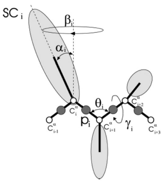
The UNRES model of the polypeptide chain. Dark circles represent united peptide groups (p) and open circles represent the C^α atoms. Ellipsoids represent side chains, with their centers of mass at the SCs. The ps are located halfway between two consecutive C^α atoms. The virtual-bond angles, θ, the virtual-bond dihedral angles, γ, and the angles, α_SC and β_SC, that define the location of a side chain with respect to the backbone, are also indicated.

$$\begin{array}{l}U=w_{sc}\sum _{i<j}{U}_{s{c}_{i}s{c}_j}+w_{{\mathit{\text{sc}}}_p}\sum _{i\ne j}{U}_{s{c}_i{p}_j}+w_{pp}\sum _{i<j-1}{U}_{p_i{p}_j}+\\ w_{\mathit{\text{tor}}}\sum _i{U}_{\mathit{\text{tor}}}\left({\gamma }_i\right)+w_{\mathit{\text{tord}}}\sum _i{U}_{\mathit{\text{tord}}}\left({\gamma }_i,{\gamma }_{i+1}\right)+w_b\sum _i{U}_b\left({\theta }_i\right)+\\ w_{\mathit{\text{rot}}}\sum _i{U}_{\mathit{\text{rot}}}\left({\alpha }_{s{c}_i},{\beta }_{s{c}_i}\right)\\ +\sum _{m=3}^6{w}_{\mathit{\text{corr}}}^{(m)}{U}_{\mathit{\text{corr}}}^{(m)}+w_{\mathit{\text{bond}}}\sum _i{U}_{\mathit{\text{bond}}}\left(d_i\right)+w_{ss}\sum _i{U}_{ss;i}\end{array}$$ (1)

where U_sciscj, U_scipj, and U_pipj denote the effective free energies of interaction between the side chains in water, between the side chains and the peptide groups, and between the peptide groups, respectively; U_bond, U_b, and U_rot are the effective potentials for stretching the virtual bonds, for bending the virtual-bond angles, and for the energetics of the rotameric states of virtual side chains, respectively; U_tor and U_tord are torsional and double-torsional potentials for rotation about the C^α…C^α virtual bonds; $U_{\mathit{\text{corr}}}^{(m)}$, m = 1,2,3,4, are correlation or multibody terms pertaining to coupling between backbone-local and backbone-electrostatic interactions²⁰ (where m denotes the order of correlation), and U_SS is a term accounting for the energetics of disulfide bonds.³¹ Each of these terms is multiplied by an appropriate weight, w.

The force field was initially applied to solve the proteinstructure prediction problem as that of finding the global minimum of the effective energy function. However, recently²² we realized that such an approach ignores conformational entropy and, strictly speaking, corresponds to “folding” proteins at the temperature of 0 K; therefore, we redefined²² the protein-structure prediction problem as finding the most probable conformational ensemble at temperatures below the folding-transition and above the glasstransition temperature. Moreover, because UNRES is an effective free-energy and not a potential-energy function, it should depend on temperature explicitly. By taking advantage of the cumulant expansion, this temperature dependence was introduced in our recent work²² by multiplying the energy-term weights by factors f_n(T) (where T denotes absolute temperature) defined by eq 2, where applicable

$$f_n\left(T\right)=\frac{\text{ln}\left(e^1+e^{-1}\right)}{\text{ln}\left\{exp\left[{\left(\frac{T}{T_{\mathit{\text{0}}}}\right)}^{n-1}\right]+exp\left[-{\left(\frac{T}{T_{\mathit{\text{0}}}}\right)}^{n-1}\right]\right\}}$$ (2)

where T₀ = 300 K.

2.2. Replica Exchange Method (REM)

The replica exchange algorithm based on a molecular dynamics (MD) method is called replica exchange molecular dynamics (REMD).⁹ The basic idea of REMD is to run constant temperature MD simulations on sequential replicas of the system simultaneously and independently, each replica at a different temperature {T₀,T₁,…,T_i,T_i+1,‥,.T_N}, where T_N is the maximum temperature at which an MD simulation is run. Usually, those temperatures are arranged in increasing order, e.g., T_i<T_i+1 (i = 0, 1, 2,…, N−1). After every fixed number of steps, an attempt is made to exchange temperatures of a pair of neighboring replicas (e.g., i and i+1); the velocities are rescaled following the change in temperature, and the exchange processes are then repeated during MD simulations. The neighboring replicas undergo an exchange with the acceptance given by the Metropolis criterion

$$\omega (X_i\to X_{i+1})=\{\begin{array}{c}1\\ exp(-\text{Δ})\end{array}\begin{array}{c}\text{Δ}\le 0\\ \text{Δ}>0\end{array}$$ (3)

where ω is the transition probability and

$$\text{Δ}=({\beta }_{i+1}–{\beta }_i)\left[U\left(X_i\right)–U\left(X_{i+1}\right)\right]$$ (4)

where β_i = 1/RT_i, T_i is the temperature corresponding to the ith replica (trajectory), X_i denotes the variables of the UNRES conformation of the ith replica at the attempted exchange point, and U(X_i) denotes the UNRES energy of conformation X_i. If Δ≤0, T_i and T_i+1 are exchanged; otherwise, the exchange is accepted with probability exp(−Δ). When the temperature-dependent UNRES force field is applied, eq 4 must be replaced by eq 5;²² this result is obtained directly by inserting the temperature-dependent energy function into eq 14 of ref 9.

$$\begin{array}{l}\text{Δ}=–\left[{\beta }_{i+\text{1}}U(X_{i+\text{1}},T_{i+\text{1}})–{\beta }_{i}U(X_{i+\text{1}},T_i)\right]+\\ \left[{\beta }_{i+1}U(X_i,T_{i+\text{1}})–{\beta }_{i}U(X_i,T_i)\right]\end{array}$$ (5)

The restricted free energy U(X,T) is calculated with eq 5 of ref 22.

To enhance sampling, in this study we used the multiplexing variant of REMD introduced by Rhee and Pandé¹² in which m independent replicas are simulated at each temperature; the same extension applied to serial replica exchange is described in the next section.

2.3. Serial Replica Exchange Method (SREM)

The basic idea of the serial replica exchange method is as follows. Let us assume that we know the potential energy distributions, P_n(E;T_n) at the temperatures T_n (n = 0, 1, 2,…, N). Let us perform a constant temperature molecular dynamics simulation at a temperature T_k, 0≤k≤N, for a given number of time steps, the final energy being equal to E⁰. From the energy distribution at its neighboring temperature, T_k±1 (only T_k−1 if k = N, and only T_k+1 if k = 0), we sample an energy E¹. Next, we attempt a move to this neighboring temperature, and the move is accepted or rejected according to the Metropolis criterion (eqs 3 and 4). If this move is accepted, the simulation (trajectory) is continued at the new temperature T_k±1 with velocities rescaled following the exchange of temperature; otherwise, it remains at the same temperature T_k.

Sampling an energy value from the distribution at a neighboring temperature replaces use of the energy of the conformation at a neighboring temperature in REM but does not require communication with the processor running the trajectory on a neighboring temperature, which is an obvious advantage. On the other hand, the energy distributions at all temperatures must be obtained prior to the production phase of the method which makes it an adaptive method as MUCA and, consequently, introduces an overhead to obtain the energy distribution. Moreover, when SREM is applied to the temperature-dependent UNRES force field, the acceptance probability cannot be computed from eq 5 given only the energy distributions at all temperatures; this problem is discussed in section 2.4.

Now the question is how to obtain the energy distributions to use in the SREM simulation. The algorithm described in ref 14 and also implemented in our work is as follows: (i) perform a short REM simulation to obtain the first approximate energy distribution at each temperature; (ii) with the approximate energy distributions, perform a set of simulations using SREM for a certain amount of time and collect the sampled potential energies at each temperature; (iii) update the potential energy distribution at each temperature by using the sampled potential energies in step (ii); and (iv) repeat steps (ii) and (iii) until the energy distributions converge at each temperature.

To investigate how quickly the potential energy distributions reach equilibrium, we employ the chi-square measure which is defined by eq 6

$${\chi }^2(t)=\sum _{i=1}^M\frac{{\left({\overline{P}}_i(t)-{\overline{P}}_i^{\mathit{\text{ref}}}\right)}^2}{{\overline{P}}_i^{\mathit{\text{ref}}}}$$ (6)

Where $\overline{P_i}\left(t\right)$ and ${\overline{P}}_i^{\mathit{\text{ref}}}$ are the current and the reference value, respectively, of the energy distribution at the ith bin of the energy histogram averaged over a time window of length t, and M is the number of bins in the energy distribution histogram. In this article, we use the final converged energy distributions obtained by a regular REM simulation as the reference. The energy distributions have become converged when χ²(t) becomes stationary. After the energy distributions converge, the update of the energy distributions can be stopped.

To sample the energy distribution, E, we employed the acceptance-rejection method,³² which can be summarized as follows. Suppose that we have an arbitrary probability distribution P(E;T) at temperature T. Let E^max, E^min, P^max, and P^min denote the maximum energy, the minimum energy, the maximum probability, and the minimum probability, respectively, for this energy distribution. Then a point (e^r,y) is generated randomly, where e^r is a random value between E^max and E^min, and y is a random number between P^max and P^min. If y≤P(e^r,T), then the value e^r is accepted; otherwise, it is rejected and the sampling step is repeated.

2.4. Modification of the SREM Algorithm for the UNRES Force Field

In the original SREM algorithm,¹⁴ attempts are made to move the temperature of a simulation randomly to its neighboring temperatures during the process. However, this could make the simulation move more frequently to some specific temperatures before the potential energy distributions reach equilibrium. For example, the simulations of Ala₁₀ and 1E0L using this SREM algorithm in Figure 2 show that the trajectories preferentially move to low temperatures for Ala₁₀ and to some lower temperatures for 1E0L during the updating phase. Therefore, to avoid this problem, we modified the original SREM algorithm as follows: (i) the frequency of each replica (simulation) moving (up or down) from its temperature to a neighboring temperature is updated periodically during the MD simulation and (ii) based on the “up or down” frequency for each replica, simulation (trajectory) attempts are made to move to its neighboring temperatures in favor of low frequency. In a word, the distinction between the modification of SREM and the original SREM is the different ways to move a simulation to its neighboring temperatures: the SREM with modification is based on the “up or down” frequency, whereas the original SREM is based on random selection.

Figure 2.

Temperature distributions between replicas, expressed as average number of replicas at a given temperature. (a) Ala₁₀ with the temperature-dependent force field and (b) 1E0L with the temperature-independent force field, respectively, in the SREM simulation without modification for 10 million steps. The temperature-independent and temperature-dependent runs are placed in the same figure to show that the bias problem that occurred in the old SREM algorithm is caused by the algorithm itself instead of by the assumption that U(X_i+1, T_i) is approximately equal to U(X_i+1, T_i+1)].

However, this modification gives rise to another issue: the modification may violate the detailed balance condition because a simulation is forced to exchange with its neighboring temperatures based on its exchange frequency instead of by a random choice. This feature does not downgrade the algorithm during the equilibration phase, i.e., before the energy probability distributions converge, because the detailed balance condition does not hold in SREM for non-converged energy distributions.¹⁴ However, the detailed balance condition should hold in the production phase when sampling is performed with the converged energy distributions, and the modification is, therefore, not applied in the production phase.

Another problem occurs when a temperature-dependent force field is used with the application of the SREM to UNRES. In the regular REM, eq 4 is simply replaced by eq 5 to compute the acceptance probability. However, the use of eq 5 is not straightforward when SREM is performed with a temperature-dependent force field because this requires knowledge of both U(X_i+1,T_i+1) and U(X_i+1,T_i) and, because U(X_i+1,T_i+1) is sampled from the energy distribution at temperature T_i+1, the conformation X_i+1 to which it corresponds is unknown. Consequently, we cannot compute U(X_i+1,T_i) given U(X_i+1,T_i+1). Hence, in the applications described in this paper (section 3.2), we assumed that U(X_i+1,T_i) ≈ U(X_i+1,T_i+1). To use eq 5 accurately, we would need to construct the joint (and hence multidimensional) energy distribution of all groups of energy terms that depend on temperature in the same way; then, after sampling all energy components from the distribution at T_i+1, and by taking advantage of eq 5 of ref 22, we could compute the energy at temperature T_i. The energy components fall into 4 groups as far as its temperature dependence is concerned:²²

1. Σ_i<jU_SCi(X), Σ_i≠jUsc_ipj(X), ${\sum }_{i<j-1}{U}_{{\text{p}}_i{\text{p}}_j}^{\text{VDW}}(X)$, Σ_iU_b(θ_i), Σ_iU_rot(α_SCi,β_SCi), and ${\sum }_{i=1}^{n\text{bond}}{U}_{\text{bond}}(d_i)$ are independent of temperature.

2. ${\sum }_{i<j-1}{U}_{{\text{p}}_i{\text{p}}_j}^{e1}(X)$ and ${\sum }_i{U}_{\mathrm{tor}}\left(\gamma i\right)$ are multiplied by f₂(T) of eq 2.

3. ${\text{U}}_{\text{corr}}^{\left(3\right)}\left(\text{X}\right)$, ${\text{U}}_{\text{turn}}^{\left(3\right)}\left(\text{X}\right)$, and ${\sum }_{\text{i}}{\text{U}}_{\text{tord}}\left(\gamma \text{i},\gamma \text{i}+1\right)$ are multiplied by f₃(T) of eq 2.

4. $U_{\mathrm{corr}}^{(4)}(X)$ and $U_{\text{turn}}^{(4)}(X)$ are multiplied by f₄(T) of eq 2.

However, the construction of a four-dimensional distribution of these four groups of energy components requires a much greater, prohibitively expensive, effort to obtain an acceptable convergence compared to obtaining a converged one-dimensional distribution of the total energy.

2.5. Evaluation of Thermodynamic Quantities from Replica Exchange Simulation

To compute thermodynamic quantities (such as the partition function, total energy, and heat capacity) from the results of the simulations carried out at different temperatures, the weighted histogram analysis method (WHAM)³³ was used, as described in ref 22. The expressions for the thermodynamic quantities are given by eqs 17–21 of ref 22.

2.6. Simulation Details

All UNRES/SREM MD simulations were carried out with the Berendsen thermostat,³⁴ the implementation of which in UNRES/MD has been described in our earlier papers.^27,35 Consequently, the random and stochastic forces were not included. In our earlier work,^27,35,36 we have shown that Newton's dynamics with the Berendsen thermostat leads to faster simulated folding compared to that of Langevin dynamics, which justifies its use in the present work, where the purpose of the simulations was to obtain converged thermodynamic functions and ensemble averages and not to determine the kinetics of folding. The coupling parameter for the Berendsen thermostat was assumed to be τ = 1 mtu (where mtu stands for molecular time unit, and 1 mtu = 48.9 fs), as in our earlier work.³⁵ The velocity Verlet (VV) algorithm,³⁷ with the variable time step extension developed in our earlier work,²⁸ was used, and the basic time step in integrating the equations of motion was 5 fs. The drawings of the structures of the proteins considered in this work were prepared with the MOLMOL program.³⁸

3. Results and Discussion

3.1. Test of the SREM with the Temperature-Independent UNRES Force Field

First, we tested the SREM algorithm on the 37-residue protein 1E0L³⁹ using the temperature-independent UNRES force field parametrized on 1E0L.²² As in our earlier study,²² we selected the central 28-residue fragment of this protein, which corresponds to a three-stranded β-sheet (Figure 3a).

Figure 3.

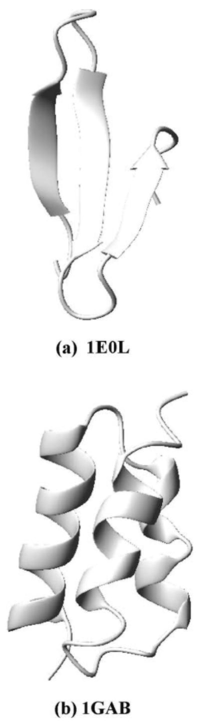
Ribbon diagrams of the experimental structures of (a) 1E0L³⁹ and (b) 1GAB.⁴⁰

To generate initial approximate UNRES energy distribution functions, we ran a regular REM simulation for 1,000,000 steps using 25 replicas over a range of temperatures from 200 to 500 K with 4 independent trajectories at each temperature. The folding-transition temperature of 1E0L with the force field used is 339 K.²² Replica exchanges were attempted every 20,000 steps during the simulation. The initial UNRES energy distributions at two representative temperatures (220 and 350 K) are plotted in Figure 4a,b. Then, 100 SREM simulations (4 independent simulations at each temperature) were performed using the initial energy distributions obtained from the short REM simulation. During the SREM simulation, the energy distributions were updated every 500,000 steps for 16,000,000 steps, after which the updated energy distributions roughly converged. A subsequent SREM simulation of another 8,000,000 steps was performed with converged energy distributions to collect the thermodynamic data. To compare the results with the REM and canonical MD, we also ran regular REM simulations and canonical MD simulations at 25 temperatures with 4 independent trajectories at each temperature for 24,000,000 steps.

Figure 4.

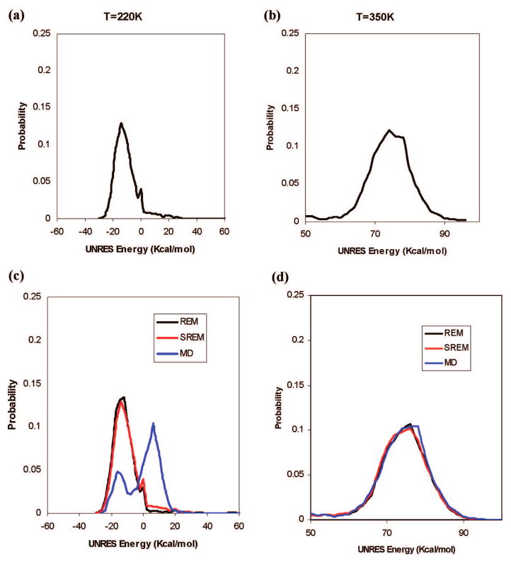
The UNRES energy distributions for 1E0L at two representative temperatures, 220 and 350 K (with the temperature-independent force field);²² curves in the top panels correspond to the initial rough UNRES energy distributions from the trial REM simulations for 1,000,000 steps at (a) 220 K and (b) 350 K; curves in the bottom panels correspond to the converged UNRES energy distributions from the REM (black), SREM (red), and canonical MD (blue) simulations at the two representative temperatures (c) 220 K and (d) 350 K.

The converged UNRES energy distributions of the SREM simulations at each temperature nearly converged to those of the REM simulations. For example, the converged UNRES energy distributions of the SREM and REM simulations at two representative temperatures (220 and 350 K) are plotted in Figure 4c,d; the black curves show the converged UNRES energy distributions obtained from the REM run, and the red curves show the converged UNRES energy distributions obtained from the SREM run. However, we observed that the converged UNRES energy distributions from the canonical MD simulations (blue curves) at low temperatures did not converge to those of the REM simulation, but they converged to those of the REM simulation only at high temperatures. For example, at T = 220 K, the plot of the converged UNRES energy distribution obtained from the canonical MD run has two peaks (one in the low-energy region and the other in the high-energy region, and the high-energy region made a major contribution to the energy distribution; Figure 4c), which means that canonical MD simulations are trapped in the high-energy region, whereas the canonical MD simulation at 350 K avoided this trapping in the high-energy region.

The convergence of the UNRES energy distributions of the REM, SREM, and canonical MD simulations was assessed quantitatively by using the χ²(t) measure defined in eq 6, at these two representative temperatures, 220 and 350 K. The values of χ²(t) are plotted against the simulation time in Figure 5. At high temperature in Figure 5b, T = 350 K, the values of χ²(t) of the canonical MD and SREM simulations have nearly converged to that of the REM simulation after 16 million steps. At lower temperature, T = 220 K, the χ² values of only the SREM simulation has converged to that of the REM simulation, but the χ² values of the canonical MD simulation has not converged to them, which confirms that the canonical MD simulation at lower temperature is trapped (see Figure 4c). To investigate the convergence properties of the SREM UNRES energy distributions at all 25 temperatures, all the simulations and the χ² values are averaged over all 25 temperatures, and the results are shown in Figure 6. The χ² result in Figure 6 shows that the convergence properties of REM and SREM are the same for all temperatures as those at two representative temperatures, 220 and 350 K (Figure 5), and the averaged result of the canonical MD simulations has not converged yet because of the poor convergence behavior at lower temperatures.

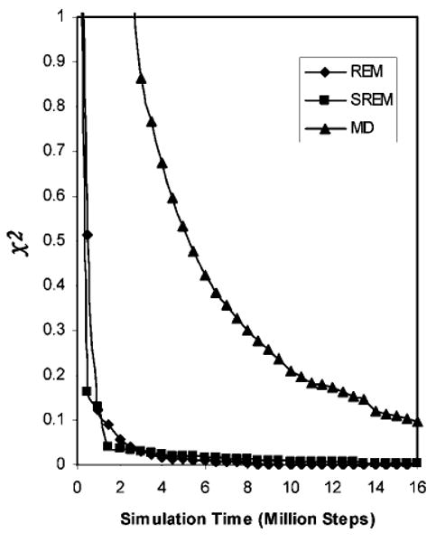
Figure 5.

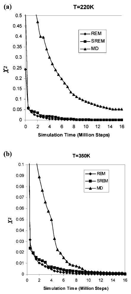
Convergence measure of the UNRES energy distributions for the REM (diamonds), SREM (squares), and canonical MD (triangles) simulations of 1E0L, at temperature (a) 220 K and (b) 350 K (with the temperature-independent force field),²² as a function of the simulation time. The χ² curves are plotted by using the converged UNRES energy distributions from the REM run for 24,000,000 steps as the reference.

Figure 6.

Convergence measure of the UNRES energy distributions for REM (diamonds), SREM (squares), and canonical MD (triangles) simulations of 1E0L as a function of the simulation time with the temperature-independent force field.²² The χ² curves are plotted by using the converged UNRES energy distributions from the regular REM run for 24,000,000 steps as the reference, and the χ² values are averaged over 25 temperatures.

To investigate the thermodynamic properties in these simulations, we have plotted heat-capacity curves. The ensemble averages of the heat capacity calculated from SREM, REM, and canonical MD simulations converge in 20,000,000 steps. The heat capacities, calculated for these simulations with 4 million consecutive steps/trajectories, are shown in Figure 7a-c. When the results of the converged heat capacities obtained from the REM, SREM, and canonical MD simulations were compared, it was observed that the two heat capacity curves of the REM and SREM nearly fit to each other, whereas the heat capacity curve of the canonical MD is obviously shifted from these curves (in Figure 7d).

Figure 7.

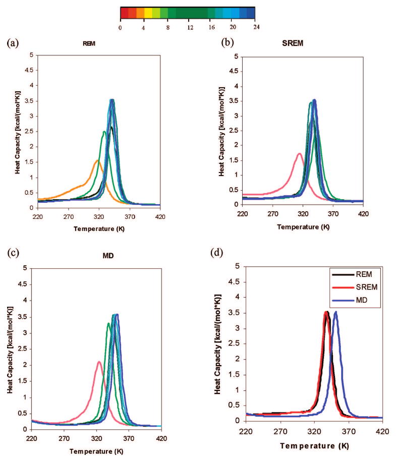
Plots of heat capacity using 4,000,000 MD consecutive steps/trajectory windows taken from (a) the REM run, (b) the SREM run, and (c) the canonical MD run of 1E0L with the optimized force field (the temperature-independent force field).²² The curves in parts (a)-(c) are colored from red to blue according to the number of MD steps; the color codes are shown in the color bar with numbers indicating the number of millions of MD steps. (d) Two converged heat capacities are obtained from the REM (black) and SREM (red) simulations, and the obvious shift of the heat capacity is obtained from the canonical MD (blue) simulation.

3.2. Test of the SREM with the Temperature-Dependent UNRES Force Field

To test the SREM with the temperature-dependent UNRES force field,²² we first chose a simple system, a ten-residue polyalanine (Ala₁₀) chain. The folding-transition temperature of Ala₁₀ with the force field used is 311 K. To obtain initial energy distribution functions, we ran a regular REM simulation (it should be noted that eq 4 is replaced by eq 5 in the regular REM run with the temperature-dependent force field) for 400,000 steps using 20 replicas over a range of temperatures from 200 to 440 K with 1 trajectory per temperature. Replica exchanges were attempted every 10,000 steps during the simulation. Then, 20 SREM simulations (1 simulation per temperature) were performed using the energy distributions obtained from the initial REM simulation. Next, the energy distributions were updated every 400,000 steps for 10,000,000 steps, at which point the UNRES energy distributions became roughly steady, which indicates that they converged. A subsequent SREM simulation of another 10,000,000 steps was performed with converged energy distributions to collect the thermo-dynamic data. To compare the SREM to the REM and the canonical MD simulations, we also ran a regular REM simulation and a canonical MD simulation at 20 temperatures also for 20,000,000 steps each with 1 trajectory per temperature.

The initial UNRES energy distributions obtained from the trial REM simulation at two representative temperatures (210 and 280 K) are plotted in Figure 8a,b. During the updating phase in the SREM simulation, the energy distributions obtained from the SREM simulation of 10,000,000 steps have nearly converged to those of the REM simulation (see Figure 8c,d). The results show that the converged UNRES energy distributions of the REM, MD, and SREM simulations, at low and high temperatures, fit each other very well, and no trapping problem was observed in the MD runs at other low temperatures.

Figure 8.

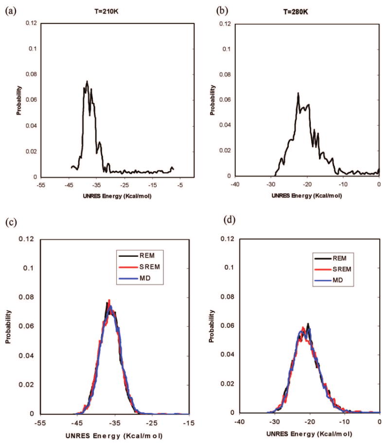
The UNRES energy distributions for Ala₁₀ at two representative temperatures, 210 and 280 K (with the temperature-dependent force field):²² curves in the top panels correspond to the initial rough UNRES energy distributions for the trial REM simulation for 400,000 steps at temperatures (a) 210 K and (b) 280 K. Curves in the bottom panels correspond to the converged UNRES energy distributions at temperatures (c) 210 K and (d) 280 K obtained from the REM (black), SREM (red), and canonical MD (blue) simulations.

The convergence properties of the energy distributions obtained from the REM, SREM, and canonical MD simulations, by using the χ²(t) measure, defined in eq 6, were assessed quantitatively at two representative temperatures, 210 and 280 K. Plots of χ²(t) against simulation time are shown in Figure 9. From Figure 9, it is observed that the χ² values for SREM and canonical MD at temperatures 210 and 280 K converge very well to those of the REM. The convergence properties of the energy distributions obtained from SREM, canonical MD, and REM, averaged over 20 temperatures, are shown in Figure 10, which illustrates the same behavior (averaged over all temperatures) as those at the two representative temperatures, 210 and 280 K (Figure 9).

Figure 9.

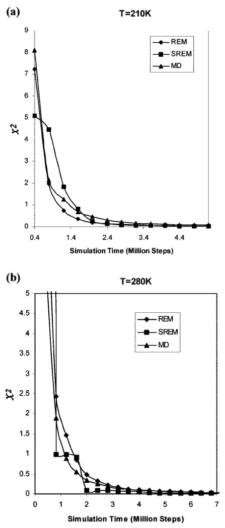
Convergence measure of the UNRES energy distributions for the REM (diamonds), SREM (squares), and canonical MD (triangles) simulations of Ala₁₀ at temperatures (a) 210 K and (b) 280 K, as a function of the simulation time with the temperature-dependent force field.²² The χ² curves are plotted by using the converged UNRES energy distributions from the regular REM run for 20,000,000 steps as the reference.

Figure 10.

Convergence measure of the UNRES energy distributions for the REM (diamonds), SREM (squares), and canonical MD (triangles) simulations of Ala₁₀ as a function of the simulation time with the temperature-dependent force field.²² The χ² curves are plotted by using the converged UNRES energy distributions from the regular REM run for 20,000,000 steps as the reference, and the χ² values are averaged over all 20 temperatures.

To investigate the thermodynamic properties from these simulations, heat-capacity curves for Ala₁₀ were plotted. Heat capacities were calculated for those simulations using 2 million consecutive steps per trajectory, which are shown in Figure 11a-c. The ensemble averages of the heat capacity calculated from the SREM, REM, and canonical MD converged in 12,000,000 steps. When the results of the converged heat capacities obtained from REM, SREM, and canonical MD simulations were compared, it was observed that the three heat capacities for REM, MD, and SREM fit each other very well (as shown in Figure 11d).

Figure 11.

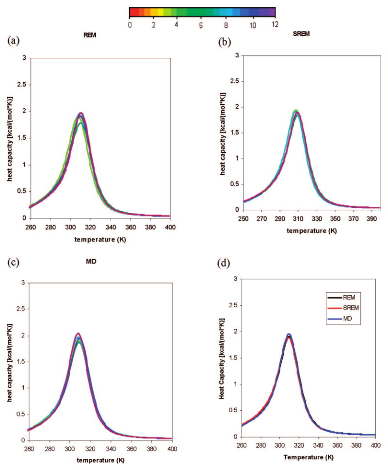
Plots of heat capacity using 2,000,000 consecutive MD steps per trajectory taken from (a) the REM run, (b) the SREM run, and (c) the canonical MD run of Ala₁₀ with the temperature-dependent force field.²² The curves in parts (a)-(c) are colored from red to blue according to the number of MD steps; the color codes are shown in the color bar with numbers indicating the number of millions of MD steps. (d) Three separate converged heat capacities obtained from the REM (black), SREM (red), and canonical MD (blue) simulations.

However, the Ala₁₀ system is a simple one, so that even canonical MD simulations give as good results as REM does with the temperature dependent force field. Hence, we tried to test SREM on a more complex protein system, 1GAB (see Figure 3b), but we were not able to obtain good results, as shown in Figures 12 and 13. From Figure 12, it is observed, at low temperature (i.e., T = 220 K), that the maximum of the UNRES energy distribution obtained from SREM is shifted to higher energies compared to that obtained from REM, while the plot of the UNRES energy distribution obtained from the canonical MD run has two peaks (one in the low-energy region and the other in the high-energy region, and the high-energy region made a major contribution to the energy distribution; Figure 12a). The χ² result in Figure 12b shows that the averaged results of the SREM and the canonical MD simulations have not converged to that of the REM simulation because of the poor convergence behavior at lower temperatures. Heat capacities were calculated for those simulations using 4 million consecutive steps per trajectory, which are shown in Figure 13a-c. The ensemble average of the heat capacity calculated from the REM converges in 12,000,000 steps, but the results from the SREM and canonical MD did not converge even in 20,000,000 steps. From Figure 13d, the heat capacities obtained from the SREM and canonical MD simulations for 20,000,000 steps have broad and multiple peaks around the transition temperature.

Figure 12.

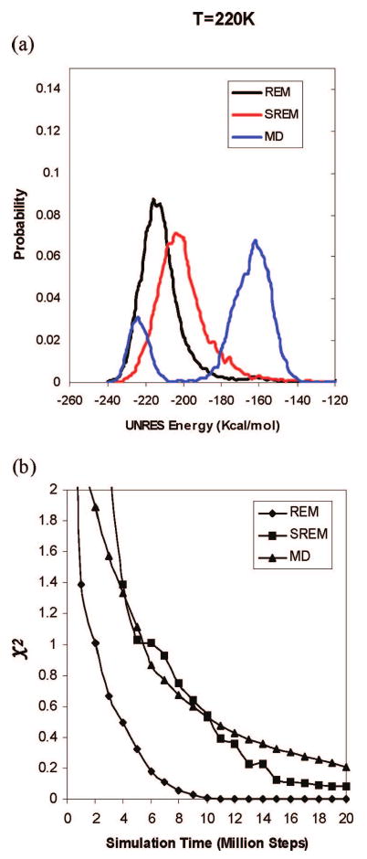
(a) The UNRES energy distribution for 1GAB at a temperature 220 K with the temperature-dependent force field.²² The black, red, and blue curves show the UNRES energy distributions obtained from the REM, SREM, and canonical MD simulations for 20 million steps, respectively. (b) Convergence measure of the UNRES energy distributions for the REM (diamonds), SREM (squares), and canonical MD (triangles) simulations of 1GAB as a function of the simulation time. The χ² curves are plotted by using the converged UNRES energy distributions from the regular REM run for 20,000,000 steps as the reference, and the χ² values are averaged over all 20 temperatures.

Figure 13.

Plots of heat capacity using 4,000,000 consecutive MD steps per trajectory taken from (a) the REM run, (b) the SREM run, and (c) the canonical MD run of 1GAB with the temperature-dependent force field.²² The curves in parts (a)-(c) are colored from red to blue according to the number of MD steps; the color codes are shown in the color bar with numbers indicating the number of millions of MD steps. (d) Three separated heat capacities obtained from the REM (black), SREM (red), and canonical MD (blue) simulations.

Therefore, SREM has failed to reproduce the thermodynamics of folding of 1GAB with the temperature-dependent UNRES force field because of the invalid calculation of the acceptance probability in eq 4 for SREM. Apparently, the assumption that U(X_i+1, T_i) ≈ U(X_i+₁,T_i+₁) (see section 2.4) works for the simple Ala₁₀ system but does not work for a more complicated 1GAB system. As mentioned in section 2.4, accurate application of eq 5 would require the determination of a four-dimensional distribution of the UNRES energy components which share the same temperature dependence. Consequently, the advantage of minimizing the cost of communication between processors in the SREM algorithm is overwhelmed by the additional cost to obtain a converged distribution of energy components. Therefore, SREM is applicable only to our temperature-independent UNRES force field.

3.3. Parallel Performance of SREM

To check the performance of SREM, we compared it with REM under the same simulation conditions. During the simulation of 1E0L with a temperature-independent UNRES force field, REM and SREM were run for 20 million steps, and REM spent 10706 s while SREM used 9929 s to finish. During the simulation of polyalanine (Ala₁₀) with the temperature-dependent UNRES force field, REM and SREM were run for 20 million steps, and REM spent 101820 s while SREM used 99864 s to finish.

We also carried out a benchmark assessment of the SREM code using the Cray XT3 computer at the Pittsburgh Supercomputer Center. Weak scaling data, obtained by holding the per-node computational work constant (500,000 steps of MD) for SREM simulations (UNRES/SREM) using the Ala₁₀ system, are presented. For comparison, a set of regular REM simulations (UNRES/REM) carried out using the Cray XT3 computer with synchronization for the same system (Ala₁₀) is presented. Those data are given in Table 1, which shows that the time (i.e., setup time, total time, and nonsetup time) of the SREM simulations and REM simulations changes with a given number of processors. Nonsetup time in the table is the difference between the total time and the setup time. It is straightforward to compare the parallel performance of the SREM simulations and regular REM by plotting the nonsetup time of the simulations against the number of processors (see Figure 14). From the results (Table 1 and Figure 14), we observe that the nonsetup time of the SREM simulations increases slightly with increasing number of processors, whereas the nonsetup time of the REM simulations increases significantly with increasing number of processors. Speedup curves, calculated from the weak scaling data in Table 1 by applying eq 7, are shown in Figure 15

Table 1.

Weak Scaling Data of UNRES REM and UNRES SREM for Ala₁₀ Using the Cray XT3 Computer at the Pittsburgh Supercomputer Center

	UNRES/REM			UNRES/SREM
no. of processors	setup time [s]	total time [s]	nonsetup time [s]	setup time [s]	total time [s]	nonsetup time [s]
4	0.14	67.15	67.01	0.16	88.57	88.41
8	0.17	66.75	66.58	0.17	88.35	88.18
16	0.24	68.11	67.87	0.24	87.51	87.27
32	0.40	67.52	67.12	0.47	88.17	87.70
64	0.61	68.77	68.16	0.66	89.85	89.19
128	1.07	69.75	68.68	1.15	88.73	87.58
256	2.05	73.87	71.82	2.29	89.28	86.99
512	3.94	78.74	74.80	4.20	94.99	90.79
1024	7.64	94.14	86.50	8.65	97.58	88.93

Figure 14.

Plots of the weak scaling data, probed by holding the per-node computational work constant for Multiplexing Replica Exchange Molecular Dynamics (REM, squares) and Serial Replica Exchange Molecular Dynamics (SREM, triangles) codes using the Cray XT3 computer.

Figure 15.

Speedup plots for Replica Exchange Molecular Dynamics (REM, squares) and Serial Replica Exchange Molecular Dynamics (SREM, triangles) codes using the Cray XT3 computer.

$$s\left(4n\right)=4n\frac{t_{n–s}(4)}{t_{n–s}(4n)}$$ (7)

where s(4n) and t_n-s(4n) are the speed-up and the nonsetup time with 4n processors, respectively, given the same per-processor work load; the calculations were always carried out with a multiple of 4 processors.

We found that the increasing number of processors does not affect the efficiency of SREM but does decrease the efficiency of regular REM, which is shown in Figure 15. Therefore, we can conclude that the parallel performance for SREM is better than that for regular REM at this time.

4. Conclusions

We have implemented UNRES/SREM and tested it on three systems: 1E0L with the temperature-independent and Ala₁₀ and 1GAB with the temperature-dependent force fields. By checking the convergence properties of the energy distributions and the thermodynamic properties of 1E0L, calculated from REM and SREM, we have demonstrated that SREM can reproduce the results of REM, while the canonical MD cannot, which means that the SREM algorithm is comparable to regular REM with the temperature-independent UNRES force field. For two simple systems studied, 1E0L and Ala₁₀, SREM turned out to be more efficient than REM. However, the data from section 3.3 indicate that the gain in wall-clock time is rather incremental than substantial. Moreover, SREM has the adaptive phase in which energy distributions are constructed, which can take a long time for a larger system.

With the temperature-dependent UNRES force field, SREM can be applicable to some simple systems such as Ala₁₀, but Ala₁₀ is so simple that MD simulations can reproduce the same results as that of REM. To check the performance of SREM with our temperature-dependent UNRES force field, we used 1GAB as the target, but SREM failed to produce good results for this protein because of too-crude an estimation of the acceptance probability under the necessary assumption that the change of the effective energy can be neglected when moving from a current temperature to a neighboring temperature. SREM showed the same poor convergence behavior as canonical MD (Figures 12 and 13). One possible solution would be to use the distribution of groups of energy terms which share common temperature dependences instead of the distribution of energy. This modification would, however, kill the advantage of the SREM algorithm over the regular REM algorithm because of the enormous amount of time required to obtain a converged multidimensional distribution of energy components. Another possible solution is to create a database of [E(T_i-1), E(T_i), E(T_i+1)] triples instead of an energy distribution to sample an energy and translate it to the energy at a neighboring temperature; this is correct in principle, but a problem here might be the large size of such a database. Assuming that 20 trajectories are run at different temperatures, and 500 most recent snapshots are saved from each (as in our study), giving 30,000 energy values to store, which is a reasonable size, this database will grow rapidly with the number of trajectories and number of snapshots to store, which is often necessary to treat larger systems. Therefore, SREM can be applied in a straightforward way only with our temperature-independent UNRES force field but not with our temperature-dependent one.

References

- 1.Wolynes PG, Onuchic JN, Thirumalai D. Science. 1995;267:1619–1620. doi: 10.1126/science.7886447. [DOI] [PubMed] [Google Scholar]
- 2.Hansmann UHE, Okamoto Y. J Comput Chem. 1997;18:920–933. [Google Scholar]
- 3.Swendsen RH, Wang JS. Phys Rev Lett. 1986;57:2607–2609. doi: 10.1103/PhysRevLett.57.2607. [DOI] [PubMed] [Google Scholar]
- 4.Geyer CJ, Thompson EA. J Am Stat Assoc. 1995;90:909–920. [Google Scholar]
- 5.Hukushima K, Nemoto K. J Phys Soc Jpn. 1996;65:1604–1608. [Google Scholar]
- 6.Tesi MC, van Rensburg EJJ, Orlandini E, Whittington SG. J Stat Phys. 1996;82:155–181. [Google Scholar]
- 7.Marinari E, Parisi G, Ruiz-Lorenzo JJ. In: Spin Glasses and Random Fields. Young AP, editor. World Scientific; Singapore: 1998. pp. 58–98. [Google Scholar]
- 8.Hansmann UHE. Chem Phys Lett. 1997;281:140–150. [Google Scholar]
- 9.Sugita Y, Okamoto Y. Chem Phys Lett. 1999;314:141–151. [Google Scholar]
- 10.García AE, Sanbonmatsu KY. Proteins. 2001;42:345–354. doi: 10.1002/1097-0134(20010215)42:3<345::aid-prot50>3.0.co;2-h. [DOI] [PubMed] [Google Scholar]
- 11.Liu P, Kim B, Friesner RA, Berne BJ. Proc Natl Acad Sci USA. 2005;102:13749–13754. doi: 10.1073/pnas.0506346102. [DOI] [PMC free article] [PubMed] [Google Scholar]
- 12.Rhee YM, Pandé VS. Biophys J. 2003;84:775–786. doi: 10.1016/S0006-3495(03)74897-8. [DOI] [PMC free article] [PubMed] [Google Scholar]
- 13.Rodinger T, Howell PL, Pomes R. J Chem Theory Comput. 2006;2:725–731. doi: 10.1021/ct050302x. [DOI] [PubMed] [Google Scholar]
- 14.Hagen M, Kim B, Liu P, Friesner RA, Berne BJ. J Phys Chem B. 2007;111:1416–1423. doi: 10.1021/jp064479e. [DOI] [PMC free article] [PubMed] [Google Scholar]
- 15.Liwo A, Pincus MR, Wawak RJ, Rackovsky S, Scheraga HA. Protein Sci. 1993;2:1697–1714. doi: 10.1002/pro.5560021015. [DOI] [PMC free article] [PubMed] [Google Scholar]
- 16.Liwo A, Pincus MR, Wawak RJ, Rackovsky S, Scheraga HA. Protein Sci. 1993;2:1715–1731. doi: 10.1002/pro.5560021016. [DOI] [PMC free article] [PubMed] [Google Scholar]
- 17.Liwo A, Ołdziej S, Pincus MR, Wawak RJ, Rackovsky S, Scheraga HA. J Comput Chem. 1997;18:849–873. [Google Scholar]
- 18.Liwo A, Ołdziej S, Pincus MR, Wawak RJ, Rackovsky S, Scheraga HA. J Comput Chem. 1997;18:874–887. [Google Scholar]
- 19.Liwo A, Kazmierkiewicz R, Czaplewski C, Groth M, Ołdziej S, Wawak RJ, Rackovsky S, Pincus MR, Scheraga HA. J Comput Chem. 1998;19:259–276. [Google Scholar]
- 20.Liwo A, Czaplewski C, Pillardy J, Scheraga HA. J Chem Phys. 2001;115:2323–2347. [Google Scholar]
- 21.Liwo A, Arlukowicz P, Czaplewski C, Ołdziej S, Pillardy J, Scheraga HA. Proc Natl Acad Sci USA. 2002;99:1937–1942. doi: 10.1073/pnas.032675399. [DOI] [PMC free article] [PubMed] [Google Scholar]
- 22.Liwo A, Khalili M, Czaplewski C, Kalinowski S, Ołdziej S, Wachucik K, Scheraga HA. J Phys Chem B. 2007;111:260–285. doi: 10.1021/jp065380a. [DOI] [PMC free article] [PubMed] [Google Scholar]
- 23.Ołdziej S, Kozłowska U, Liwo A, Scheraga HA. J Phys Chem A. 2003;107:8035–8046. [Google Scholar]
- 24.Liwo A, Ołdziej S, Czaplewski C, Kozłowska U, Scheraga HA. J Phys Chem B. 2004;108:9421–9438. [Google Scholar]
- 25.Ołdziej S, Liwo A, Czaplewski C, Pillardy J, Scheraga HA. J Phys Chem B. 2004;108:16934–16949. [Google Scholar]
- 26.Ołdziej S, Lagiewka J, Liwo A, Czaplewski C, Chinchio M, Nanias M, Scheraga HA. J Phys Chem B. 2004;108:16950–16959. [Google Scholar]
- 27.Ołdziej S, Czaplewski C, Liwo A, Chinchio M, Nanias M, Vila JA, Khalili M, Arnautova YA, Jagielska A, Makowski M, Schafroth HD, Kazmierkiewicz R, Ripoll DR, Pillardy J, Scheraga HA. Proc Natl Acad Sci USA. 2005;102:7547–7552. doi: 10.1073/pnas.0502655102. [DOI] [PMC free article] [PubMed] [Google Scholar]
- 28.Khalili M, Liwo A, Rakowski F, Grochowski P, Scheraga HA. J Phys Chem B. 2005;109:13785–13797. doi: 10.1021/jp058008o. [DOI] [PMC free article] [PubMed] [Google Scholar]
- 29.Kubo R. J Phys Soc Jpn. 1962;17:1100–1120. [Google Scholar]
- 30.Kolinski A, Skolnick J. J Chem Phys. 1992;97:9412–9426. [Google Scholar]
- 31.Chinchio M, Czaplewski C, Liwo A, Ołdziej S, Scheraga HA. J Chem Theory Comput. 2007;3:1236–1248. doi: 10.1021/ct7000842. [DOI] [PubMed] [Google Scholar]
- 32.Robert CP, Casella G. Monte Carlo Statistical Methods. Springer; New York: 1999. Monte Carlo Integration; pp. 92–96. [Google Scholar]
- 33.Kumar S, Bouzida D, Swendsen RH, Kollman PA, Rosenberg JM. J Comput Chem. 1992;13:1011–1021. [Google Scholar]
- 34.Berendsen HJC, Postma JPM, van Gunsteren WF, DiNola A, Haak JR. J Chem Phys. 1984;81:3684–3690. [Google Scholar]
- 35.Khalili M, Liwo A, Jagielska A, Scheraga HA. J Phys Chem B. 2005;109:13798–13810. doi: 10.1021/jp058007w. [DOI] [PMC free article] [PubMed] [Google Scholar]
- 36.Liwo A, Khalili M, Scheraga HA. Proc Natl Acad Sci USA. 2005;102:2362–2367. doi: 10.1073/pnas.0408885102. [DOI] [PMC free article] [PubMed] [Google Scholar]
- 37.Swope WC, Andersen HC, Berens PH, Wilson KR. J Chem Phys. 1982;76:637–649. [Google Scholar]
- 38.Koradi R, Billeter M, Wüthrich K. J Mol Graph. 1996;14:51–55. doi: 10.1016/0263-7855(96)00009-4. [DOI] [PubMed] [Google Scholar]
- 39.Macias MJ, Gervais V, Civera C, Oschkinat H. Nat Struct Biol. 2000;7:375–379. doi: 10.1038/75144. [DOI] [PubMed] [Google Scholar]
- 40.Johansson MU, de Chateau M, Wikstrom M, Forsen S, Drakenberg T, Bjorck L. J Mol Biol. 1997;266:859–865. doi: 10.1006/jmbi.1996.0856. [DOI] [PubMed] [Google Scholar]