Computer-Aided Renal Cancer Quantification and Classification from Contrast-enhanced CT via Histograms of Curvature-Related Features

Abstract

In clinical practice, renal cancer diagnosis is performed by manual quantifications of tumor size and enhancement, which are time consuming and show high variability. We propose a computer-assisted clinical tool to assess and classify renal tumors in contrast-enhanced CT for the management and classification of kidney tumors. The quantification of lesions used level-sets and a statistical refinement step to adapt to the shape of the lesions. Intra-patient and inter-phase registration facilitated the study of lesion enhancement. From the segmented lesions, the histograms of curvature-related features were used to classify the lesion types via random sampling. The clinical tool allows the accurate quantification and classification of cysts and cancer from clinical data. Cancer types are further classified into four categories. Computer-assisted image analysis shows great potential for tumor diagnosis and monitoring.

I. INTRODUCTION

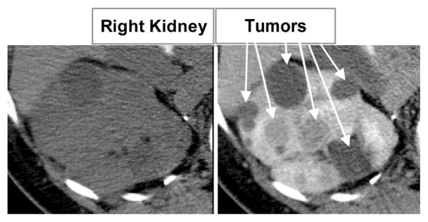
It is estimated that a quarter of a million people in the USA are living with kidney cancer and their number increases by 51000 yearly [11]. Contrast-enhanced CT has proven exceptionally useful to improve diagnosis due to the ability to differentiate tumors from healthy kidney tissue [2,23]. Fig. 1 shows an example of how normal kidney parenchyma and lesions change intensity in contrast-enhanced CT. The level of enhancement in a tumor is an crucial indicator of malignancy; equally important is the growth/regression rate of tumors for a well targeted therapy.

Fig. 1.

Multi-phase abdominal 4D CT data. 2D slices of 3D volumes: (a) before contrast and (b) at portal venous enhancement phase.

As manual measurements are time consuming and show high intra- and inter-operator variability, computer-assisted radiology shows great promise in assisting the monitoring of renal tumors. Moreover, the two-dimensional (2D) bias toward the image acquisition plane manifested during the manual measurement of cancer can be removed by the 3D quantification allowed by computer analysis.

Most work in renal image analysis is related to kidney segmentation [3,9,15,18]. The quantification and classification of kidney tumors was seldom addressed. Notably, a marker-controlled watershed algorithm segmented both renal and lesion volumes in 2D data using three manual contours and granulometry [19]. A homogeneous region growing from a seed point was presented in [10].

Recently, feature extraction from statistical information of basic image descriptors showed promising results in image processing and computer vision applications. Image features may include edge and gradient descriptors. Representative methods include Scale-Invariant Feature Transform (SIFT) [13], Shape Context [1] and Histograms of Oriented Gradient (HOG) [6]. Inspired by HOG, in this paper we propose using a set of shape descriptors called Histograms of Curvature Features (HCF) to describe renal lesions for cancer classification. HCF was previously used for colon polyp matching [21]; we employ it to classify renal tumors. HCFs are statistical descriptors that can capture the intrinsic properties of lesions. We utilize multi-phase CT values and curvature-related descriptors as basic image descriptors, i.e. shape index, curvedness, Gaussian and mean curvatures. The advantage of these curvature related descriptors is that they are rotation, translation and scale invariant. After feature extraction, non-linear dimensionality reduction is applied to HCF features to characterize lesions.

Our study proposes the semi-automated quantification and classification of renal tumors for the assertive management of tumor diagnoses and monitoring. First, it quantified the three-dimensional size, volume and enhancement of renal tumors. Then, combined histograms of curvature-related features and lesion intensity were used to classify the lesion types via random sampling. This is, to our knowledge, the first semi-automated method that quantifies and classifies renal tumors using serial enhancement.

II. Materials and Methods

A. Data and Materials

Contrast-enhanced CT data consisted of two serial acquisitions. The first image was obtained before contrast administration. Then the patients were injected with 130ml of Isovue-300 and a contrast-enhanced acquisition was completed during the portal venous phase. Data were collected using LightSpeed Ultra and QX/i (GE Healthcare) and MX 8000 scanners (Philips Healthcare). Image resolution ranged from 0.64×0.64 mm² to 0.97×0.97mm² in the axial plane with 1 mm slice thickness.

Data from 40 patients with renal tumors were analyzed with a total of 116 lesions. Lesion diameter varied from 5.3 to 43.3 mm. There were 41 cysts and 75 cancers: 22 Von Hippel-Lindau (VHL) syndromes, 13 Birt-Hogg-Dube (BHD) syndromes, 19 hereditary papillary renal cell (HPRC) carcinomas, and 21 hereditary leiomyomatosis and renal cell cancers (HLRCC). Twelve lesions of mixed types were segmented manually by two observers.

The method for lesion analysis can be subdivided into two major steps: quantification and classification via HCF.

B. Segmentation/Quantification

The segmentation and quantification of tumors follows the algorithm in [12]. Lesions were segmented in the venous phase, when they appear better differentiated from the enhanced renal tissue. Data from the two-phase scans are first automatically aligned by the image position relative to the body. The pre-processing of images includes an intra-patient inter-phase registration and data smoothing. The Perona-Malik anisotropic diffusion [16] was employed for smoothing and the demons non-linear algorithm for registration [20]. The images before contrast enhancement were registered to the venous phase data. Although the contrast-enhanced CT data are intra-modal, the organ enhancement requires the use of a multimodal similarity measure, e.g. mutual information [14].

The segmentation of renal lesions used a combination of fast marching and geodesic active contour level sets [5,17]. A fast marching level set initializes the segmentation expanding from a seed point provided by the user. The sigmoid of the gradients computed from the portal venous phase CT scan supplied the edge image. Then, a level set based on geodesic active contours refines the fast marching segmentation [5]. The level set parameters were automatically adapted to image characteristics for segmentation robustness [12].

The quantification allows computing linear and volumetric measurements of a lesion from its segmentation. Moreover, the lesions’ volumes and CT values can be extracted for subsequent classification.

C. Histograms of Curvature-related Features

Renal lesions appear to be spherical with smooth surfaces. However, their shape may be influenced by the location in/on the kidney, the solidity of the tumor, and the properties of the surrounding tissue. Most importantly, the CT values characterizing the lesion at different stages of the contrast enhancement are key features for the characterization of tumors. Hence, we propose computing histograms that combine morphological and multi-phase (4D) intensity (including enhancement) features for each lesion to classify cysts and types of cancer.

Intuitively, curvature measures the extent that a geometric object deviates from flat. For a two-dimensional iso-surface embedded in R³, the intersection of the surface with a plane containing the normal vector and one of the tangent vectors at a point on the surface is a plane curve and has a curvature called normal curvature. The maximum and minimum values of the normal curvature at a point are called the principal curvatures, k₁ and k₂. The directions of the corresponding tangent vectors are called principal directions. The Gaussian curvature is defined as the product of the principal curvatures: k_Gaussian=k₁k₂. A surface is locally convex when the Gaussian curvature is positive; it is locally saddle when the Gaussian curvature is negative. The mean curvature is one-half of the sum of the principal curvatures: k_mean=(k₁+k₂)/2. Besides Gaussian and mean curvatures [8], shape index (SI) and curvedness (CV) can also describe the shape of a lesion [22]. At a given voxel p, SI and CV features can be defined as

$$\begin{array}{l}SI(p)=\frac{1}{2}-\frac{1}{\pi }arctan\frac{k_1(p)+k_2(p)}{k_1(p)-k_2(p)}\\ CV(p)=\sqrt{\left({k_1}^2(p)+{k_2}^2(p)\right)/2};\end{array}$$

where k₁(p)>k₂(p) are two principal curvatures.

To make full use of curvature information and capture internal texture information of renal lesions, we utilize histograms of curvature features to characterize the tumors. In Table I, we list seven curvature-related features (including the gradient magnitude) used in our HCF method. Additionally, a feature based on the CT values (here CT value = Hounsfield units + 1024) was used to help to characterize lesions. For each feature, we choose a range and divide it into 98 equally-spaced bins. Voxels whose feature values are smaller than the lower limit or larger than the upper limit are counted in two additional bins. We concatenate the eight histograms and get a feature vector with 800 dimensions for each lesion for each phase. The size of the curvature computation kernel had σ=5.

TABLE I.

Features used by the HCF descriptor

	Lower limit	Upper limit
Shape index	0	+1
Curvedness	0	+1
Gaussian curvature	−1	+1
Mean curvature	−1	+1
Max curvature	−1	+1
Min curvature	−1	+1
Gradient magnitude	0	300
CT value	0	1500

Lower and upper limits are listed for each feature used in the histograms. These limits are selected according to the distributions of features. The number of bins used for each feature was 100.

Due to the large number of features and limited sample data, it is prohibitive to learn a good decision boundary. Dimensionality reduction of data can assist training a good classifier in the low dimensional space. Principal component analysis (PCA) is a classic technique for dimensionality reduction [7]. It is an orthogonal linear transformation in essence and projects the data to a new coordinate system with low dimensions which can retain the variance of original data to the maximum extent. Given a dataset which contains n samples X = {x₁, x₂,…, x_n}, PCA finds the first q principal axes w_j, j = {1,…,q} which are orthonormal and can retain variance of samples to maximal extent. The principal vectors are given by the q dominant eigenvectors of the sample covariance matrix $S=1/N{\sum }_n\left(x_n-\overline{x}\right){\left(x_n-\overline{x}\right)}^T$, where x̄ is the data sample mean. The q principal components of the observed samples x_n are given through linear mapping t_n = W^T(x_n − x̄), where W = {w₁, w₂,…, w_q}

After PCA dimension reduction, the kidney data were mapped into a 10 dimensional linear subspace according to the distribution of eigenvalues. Random sampling was used to train and test the algorithm and a support vector machine [4] to perform the classification.

Comparative tests using only the mean CT value of a lesion at different enhancement phases were performed, as in clinical practice [23]. In our approach we used CT values before contrast enhancement and at portal venous phases.

III. Results

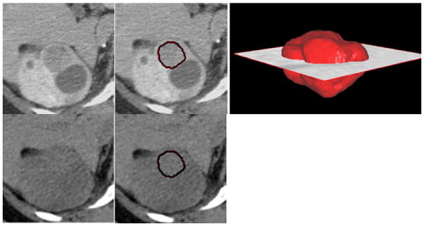
On registered data, the computer segmentations of lesions from the portal venous phase were used to estimate the mean intensity of lesions in the non-contrast phase. Fig. 2 shows an example of multi-phase segmentation of lesions. Although there is insufficient intensity information for the direct segmentation of tumors from the non-contrast phase, our method allows their accurate quantification.

Fig. 2.

Segmentation of renal lesions. The top row shows a VHL tumor segmented in the portal venous phase and its 3D rendering. The bottom row presents the segmentation from the non-contrast data. Note the irregular shape of this cancer.

The inter-observer manual measurements of lesions showed a volume overlap of 0.8±0.06, while the overlaps between the computer segmentation and each of the observers were 0.8±0.06 and 0.8±0.05 respectively.

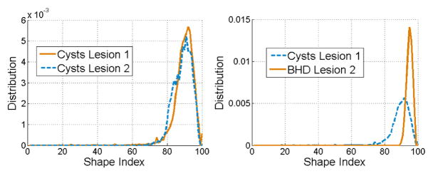
Fig. 3 shows the distribution of SI as an example of feature selection for lesion classification. Although a priori lesions are approximately spherical, this is not a generally valid assumption, as seen in the rendering in Fig. 2. Note in Fig. 3 the similarities between SI distributions of two cysts versus the morphological discrepancies between a benign and a malignant lesion. Using HCF, these structural differences are quantifiable to classify between cysts and cancers.

Fig. 3.

Distribution of shape indexes between two benign lesions (left) and a benign and malignant lesion (right).

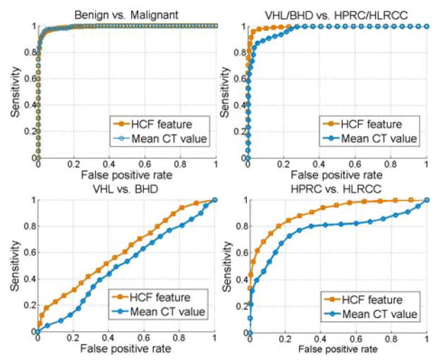
Based on clinical observations of renal tumors in CT [23], we analyzed the patterns of tumor enhancement to differentiate between different types of lesions. The enhancement analysis was compared to the HCF classification, which encompassed both 4D intensity and morphological information. Fig. 4 shows the receiver operating characteristic (ROC) curves for classifying renal lesions. Each point on the ROC is the average result of 50 random tests. First, we separate benign and malignant lesions. Then VHL/BHD cancers (typically solid tumors) are separated from HPRC/HLRCC. Finally, all categories of cancers are classified into VHL, BHD, HPRC and HLRCC. Areas under the curve (AUC) were computed for the results shown in Fig. 4 and ROC curves using HCF were compared with those obtained from employing only the mean CT values of lesions. Statistical results are presented in Table II. The sensitivity and specificity of tumor classification are reported using HCF.

Fig. 4.

Classification ROC curves using HCF vs. mean multi-phase CT values.

TABLE II.

ROC analys for the classification of renal lesions

	AUC-HCF	AUC-CT	SE (%)	SP (%)
Benign vs. malignant (p= 0.45)	0.99	0.99	97.8	93.7
VHL/BHD vs. HPRC/HLRCC (p<0.001)	0.99	0.96	97.7	93.8
VHL vs. BHD (p<0.001)	0.61	0.5	51.2	61.4
HPRC vs. HLRCC (p<0.001)	0.9	0.77	80	83.7

Areas under the curve (AUC), sensitivity (SE) and specificity (SP) values are presented for the ROC curves used to classify renal tumors. SE and SP reflect the best results obtained using HCF. p values were computed between comparative ROC curves using HCF or mean CT values.

IV. Discussion

A method for the semi-automated quantification and classification of renal tumors was presented, to assist in the clinical management of tumor diagnoses and monitoring. We quantified the 3D size and volume of renal tumors with errors comparable to the manual inter-observer variability. Additionally, our method analyzes the enhancement and morphology of segmented lesions via histograms of curvature-related features (HCF). The HCF method utilizes the distributions of various morphological features inside the lesions combined with multi-phase intensity (CT values) information. In order to capture the intrinsic dimensions of the high-dimensional HCF feature, dimensionality reduction was employed after feature extraction. Experimental results on a CTC dataset of 116 renal lesions showed that the HCF method is superior to the typical clinical method based on mean CT values. Moreover, our approach found quantifiable discrepancies between morphologies of benign and malignant lesions.

Five types of renal lesions were analyzed: benign cysts, von Hippel-Lindau (VHL) syndromes, Birt-Hogg-Dube (BHD) syndromes, hereditary papillary renal cell (HPRC) carcinomas, and hereditary leiomyomatosis and renal cell cancers (HLRCC). The automated classification of tumors showed significant separation between benign and malignant tumors and allows the further classification into types of cancer. The differentiation between VHL and BHD syndromes had the poorest results, as both types of cancer have similar appearance properties.

The automated analysis for renal tumor classification and shows great promise toward computer-assisted kidney diagnosis. The method has the potential to allow the serial analysis of tumors for disease monitoring, drug trials and noninvasive clinical surveillance.

References

- 1.Belongie S, Malik J, Puzicha J. Shape matching and object recognition using shape contexts. IEEE Tran PAMI. 2002;24 (24):509–521. [Google Scholar]
- 2.Birnbaum BA, et al. Renal cyst pseudoenhancement: influence of multidetector CT reconstruction algorithm and scanner type in phantom model. Radiology. 2007;244(3):767–775. doi: 10.1148/radiol.2443061537. [DOI] [PubMed] [Google Scholar]
- 3.Boykov YY, Jolly MP. Interactive graph cuts for optimal boundary & region segmentation of objects in N-D images. Proc of Int Conf on Comp Vision; 2001. pp. 105–112. [Google Scholar]
- 4.Burges CJC. A tutorial on support vector machines for pattern recognition. Data Mining and Knowledge Discovery. 1998;2:121–167. [Google Scholar]
- 5.Caselles V, Kimmel R, Sapiro G. Geodesic active contours. International Journal on Computer Vision. 1997;22(1):61–97. [Google Scholar]
- 6.Dalal N, Triggs B. Histograms of oriented gradients for human detection. IEEE Conf CVPR; 2005. pp. 886–893. [Google Scholar]
- 7.Jackson JE. A User’s Guide to Principal Components. New York: John Wiley & Sons; 1991. [Google Scholar]
- 8.Jerebko AK, et al. Computer-assisted detection of colonic polyps with CT colonography using neural networks and binary classification trees. Med Phys. 2003;30(1):52–60. doi: 10.1118/1.1528178. [DOI] [PubMed] [Google Scholar]
- 9.Joshi S, et al. Multiscale deformable model segmentation and statistical shape analysis using medical descriptions. IEEE Transactions on Medical Imaging. 2002;21(5):538–550. doi: 10.1109/TMI.2002.1009389. [DOI] [PubMed] [Google Scholar]
- 10.Kim DY, Park JW. Computer-aided detection of kidney tumor on abdominal computer tomography scans. Acta Radiologica. 2004;45:791–795. doi: 10.1080/02841850410001312. [DOI] [PubMed] [Google Scholar]
- 11.Linehan WM. Targeting VEGF receptors in kidney cancer. The Lancet Oncology. 2007;8(11):956–957. doi: 10.1016/S1470-2045(07)70322-4. [DOI] [PubMed] [Google Scholar]
- 12.Linguraru MG, et al. Renal tumor quantification and classification in contrast-enhanced abdominal CT. In: Pattern Recognition. 2009;42(6):1149–1161. doi: 10.1016/j.patcog.2008.09.018. [DOI] [PMC free article] [PubMed] [Google Scholar]
- 13.Lowe D. Distinctive image features from scale-invariant keypoints. Int J of Comp Vis. 2004;60(2):91–110. [Google Scholar]
- 14.Mattes D, et al. Eubank W. PET-CT image registration in the chest using free-form deformations. IEEE Tran Med Imaging. 2003;22(1):120–128. doi: 10.1109/TMI.2003.809072. [DOI] [PubMed] [Google Scholar]
- 15.Park H, Bland PH, Meyer CR. Construction of an abdominal probabilistic atlas and its application in segmentation. IEEE Transactions on Medical Imaging. 2003;22(4):483–492. doi: 10.1109/TMI.2003.809139. [DOI] [PubMed] [Google Scholar]
- 16.Perona P, Malik J. Scale-space and edge detection using anisotropic diffusion. IEEE Tran PAMI. 1990;12:629–639. [Google Scholar]
- 17.Sethian JA. Level set methods and fast marching methods: evolving interfaces in computational geometry, fluid mechanics, computer vision and materials science. Cambridge University Press; 1999. [Google Scholar]
- 18.Song T, et al. Integrated four dimensional registration and segmentation of dynamic renal MR images. Proceedings of MICCAI; LNCS. 2006. pp. 758–65. [DOI] [PubMed] [Google Scholar]
- 19.Summers RM, et al. Helical CT of Von Hippel-Lindau: semiautomated segmentation of renal lesions. Proc. of International Conference in Image Processing; 2001. pp. 293–296. [Google Scholar]
- 20.Thirion JP. Image matching as a diffusion process: an analogy with Maxwell’s demons. Med Im Analysis. 1998;2(3):243–260. doi: 10.1016/s1361-8415(98)80022-4. [DOI] [PubMed] [Google Scholar]
- 21.Wang S, Yao J, Summers RM. Matching Colonic Polyps from Prone and Supine CT Colonography Scans Based on Statistical Curvature Information. Proc ICPR; 2008. [Google Scholar]
- 22.Yoshida H, Nappi J. Three-dimensional computer-aided diagnosis scheme for detection of colonic polyps. IEEE Tran Med Imaging. 2001;20:1261–1274. doi: 10.1109/42.974921. [DOI] [PubMed] [Google Scholar]
- 23.Zhang J, et al. Solid renal cortical tumors: differentiation with CT. Radiology. 2007;244(2):494–504. doi: 10.1148/radiol.2442060927. [DOI] [PubMed] [Google Scholar]