Accuracy and run-time comparison for different potential approaches and iterative solvers in finite element method based EEG source analysis

Abstract

Accuracy and run-time play an important role in medical diagnostics and research as well as in the field of neuroscience. In Electroencephalography (EEG) source reconstruction, a current distribution in the human brain is reconstructed noninvasively from measured potentials at the head surface (the EEG inverse problem). Numerical modeling techniques are used to simulate head surface potentials for dipolar current sources in the human cortex, the so-called EEG forward problem.

In this paper, the efficiency of algebraic multigrid (AMG), incomplete Cholesky (IC) and Jacobi preconditioners for the conjugate gradient (CG) method are compared for iteratively solving the finite element (FE) method based EEG forward problem. The interplay of the three solvers with a full subtraction approach and two direct potential approaches, the Venant and the partial integration method for the treatment of the dipole singularity is examined. The examination is performed in a four-compartment sphere model with anisotropic skull layer, where quasi-analytical solutions allow for an exact quantification of computational speed versus numerical error. Specifically-tuned constrained Delaunay tetrahedralization (CDT) FE meshes lead to high accuracies for both the full subtraction and the direct potential approaches. Best accuracies are achieved by the full subtraction approach if the homogeneity condition is fulfilled. It is shown that the AMG-CG achieves an order of magnitude higher computational speed than the CG with the standard preconditioners with an increasing gain factor when decreasing mesh size. Our results should broaden the application of accurate and fast high-resolution FE volume conductor modeling in source analysis routine.

1. Introduction

Electroencephalography (EEG) based source reconstruction of cerebral activity (the EEG inverse problem) is an important tool both in clinical practice and research [35,23], and in cognitive neuroscience [2]. Methods for solving the inverse problem are based on solutions to the corresponding forward problem, i.e., the simulation of EEG potentials for a given primary source in the brain using a volume-conduction model of the human head. While the theory of this forward problem is well established and many numerical implementations exist, there remain unresolved questions regarding the accuracy and efficiency of contemporary approaches. In this study, we compared a range of numerical techniques and source representation approaches and have shown that careful choice of both are critical in order to solve realistic electroencephalographic forward (and inverse) problems.

The general approach for solving bioelectric field problems under realistic conditions is well established. All quantitative solutions for the EEG forward problem are based on the quasi-static Maxwell equations [25]. The primary sources are electrolytic currents within the dendrites of the large pyramidal cells of activated neurons in the human cortex. Even if there are also smoother models [33], most often the primary sources are formulated as a mathematical point current dipole [25,6,18]. The finite element (FE) method is often used for the solution of the forward problem, because it allows for a realistic representation of the complicated head volume conductor with its tissue conductivity inhomogeneities and anisotropies [45,3,1,34,4,15,19,37,26,39,7].

To implement the point current dipole as a current source in the brain, the FE method requires careful consideration of the singularity of the potential at the source position. One way to address the singularity is to use a subtraction approach, which divides the total potential into an analytically known singularity potential and a singularity-free correction potential, which can then be approximated numerically using an FE approach [3,1,34,15,26,41,39]. For the correction potential, the existence and uniqueness for a weak solution in a zero-mean function space have been proven and FE convergence properties are known [39]. The subtraction FE approach has thus a sound mathematical basis for point current dipole models. Another family of source representation methods, known as direct FE approaches to the total potential [45,1,4,37,26], are computationally less expensive, but also mathematically less sound under the assumption that a point dipole is the more realistic source model. In our previous work [41,44], we compared the projected subtraction approach [39] with the two direct approaches using partial integration [45,1,37] and Venant [4] in regular and geometry-adapted 2mm hexahedral FE meshes of a multi-layer sphere model for which quasi-analytical solutions exist [5]. The Venant approach was found to be the overall best choice in FE source analysis practice [41,44]. It was however speculated that an improved numerical quadrature might solve the accuracy problems of the projected subtraction approach for eccentric sources, so that the highest future potential was given to an improved implementation of the FE subtraction approach [44]. It has recently been shown that a full subtraction approach [7] using an improved numerical quadrature leads to an order of magnitude more accurate solution than the projected subtraction approach [39], especially when considering sources that are close to a conductivity inhomogeneity.

Another general prerequisite for FE modeling of bioelectric fields is the generation of a mesh that represents the geometry and electric properties of the volume conductor. An effective meshing strategy will balance acceptable forward problem accuracy against reasonable computation times and memory usage. Very high accuracies can be achieved by making use of a Constrained Delaunay Tetrahedralization (CDT) [30,29] in combination with a full subtraction approach [7]. Adaptive methods, using local refinement around the source singularity [3,34], are another potential utility but they preclude the use of fast transfer matrices [37,8,43,12] and lose efficiency in solving the inverse problem (see discussion section).

Solving the forward problem is rarely the ultimate goal in calculating bioelectric fields but rather a step towards solving the associated inverse problem. Thus the quest for numerical accuracy and efficiency of the forward solution requires some anticipation of the ultimate use in inverse solutions. The longtime state-of-the-art approach has been to solve an FE equation system for each anatomically and physiologically meaningful dipolar source (each source results in one FE right-hand side (RHS) vector) [3,1,34,4,15]. The use of standard direct (banded LU factorization for a 2D source analysis scenario [1]) or iterative (Conjugate Gradient (CG) without preconditioning [3] or Successive OverRelaxation (SOR) [26]) FE solver techniques limit the overall resolution of the geometric model because of their computational cost. The preconditioned CG method was used with standard preconditioners like Jacobi (Jacobi-CG) [37] or incomplete Cholesky without fill-in, IC(0)-CG [4].

One recent approach to achieve efficient computation of the FE-based forward problem is to pre-compute transfer matrices that encapsulate the relationship between source locations and sensor sites based only on the geometric and conductivity characteristics of the volume conductor, i.e., they are independent of the source. Techniques exist to construct transfer matrices for problem formulations based on EEG [37,12] or combined EEG and MEG [8,43]. Using this principle, for each head model, one only has to solve one large sparse FE system of equations for each of the possible sensor locations in order to compute the full transfer matrix. Each forward solution is then reduced to multiplication of the transfer matrix by an FE RHS vector containing the source load. Exploiting the fact that the number of sensors (currently up to about 600) is much smaller than the number of reasonable dipolar sources (tens of thousands), the transfer matrix approach is substantially faster than the state-of-the-art forward approach (i.e., solving an FE equation system for each source) and can be applied to inverse reconstruction algorithms in both continuous and discrete source parameter space for EEG and MEG. Still, the solution of hundreds of large linear FE equation systems for the construction of the transfer matrices is a major time consuming part within FE-based source analysis.

The first goal of this study was therefore to compare the numerical accuracy of the full subtraction approach [7] with the two direct approaches using partial integration [45,1,37] and Venant [4] in specifically-tuned CDT meshes of an anisotropic four-compartment sphere model. We then examine the interplay of the source model approaches with three FE solver methods: a Jacobi-CG, an incomplete Cholesky CG (e.g., [27]), and an algebraic multigrid preconditioned CG (AMG-CG), which has already shown to be especially suited for problems with discontinuous and anisotropic coefficients [22,32,21,9,38].

2. Theory

In the quasi-static approximation of the Maxwell equations, the distribution of electric potentials Φ in the head domain Ω of conductivity σ, resulting from a primary current j^p is governed by the Poisson equation with homogeneous Neumann boundary conditions on the head surface Γ = ∂Ω [20,25], which we can express as

$$\nabla \cdot (\sigma \nabla \Phi )=\nabla \cdot {\mathbf{j}}^p={\mathrm{J}}^p\text{in}\Omega ,\langle \sigma \nabla \Phi ,\mathbf{n}\rangle =0\text{on}\Gamma ,$$ (1)

with n the unit surface normal, and assuming a reference electrode with given potential, i.e., Φ(x_ref) = 0. The primary currents are modeled by a mathematical dipole at position ${\mathbf{x}}_0\in {\mathbb{R}}^3$ with moment ${\mathbf{M}}_0\in {\mathbb{R}}^3$ [25,6,18],

$${\mathrm{J}}^p=\nabla \cdot {\mathbf{j}}^p\left(\mathbf{x}\right)=\nabla \cdot \left({\mathbf{M}}_0\delta (\mathbf{x}-{\mathbf{x}}_0)\right),$$ (2)

where δ is the Dirac delta distribution.

2.1. Finite element modeling techniques for the potential singularity

One of the key questions for all three-dimensional EEG forward modeling techniques is the appropriate treatment of the potential singularity introduced into the differential equation by the formulation of the mathematical dipole (2). This study examined the interplay of FE solver methods (see Section 2.2) with the solution accuracy in four-layer sphere models applying three singularity treatment techniques: a full subtraction approach, a partial integration direct method and a Venant direct method.

2.1.1. Full subtraction approach

The subtraction approach [3,1,39,7] splits the total potential Φ into two parts,

$$\Phi ={\Phi }_0+{\Phi }_{\mathrm{corr}},$$ (3)

where the singularity potential, Φ₀, is defined as the solution for a dipole in an unbounded homogeneous conductor with constant conductivity σ₀. ${\sigma }_0\in {\mathbb{R}}^{3\times 3}$ is the conductivity at the source position, which is assumed to be constant in a non-empty subdomain Ω₀ around x₀, in the following called the homogeneity condition. The solution of Poisson’s equation under these conditions for the singularity potential

$$\nabla \cdot ({\sigma }_0\nabla {\Phi }_0)=\nabla \cdot {\mathbf{j}}^p$$ (4)

can be formed analytically for the mathematical dipole (2) [7] as

$${\Phi }_0\left(\mathbf{x}\right)=\frac{1}{4\pi \sqrt{\det {\sigma }_0}}\frac{\langle {\mathbf{M}}_0,{\left({\sigma }_0\right)}^{-1}(\mathbf{x}-{\mathbf{x}}_0)\rangle }{{\langle {\left({\sigma }_0\right)}^{-1}(\mathbf{x}-{\mathbf{x}}_0),(\mathbf{x}-{\mathbf{x}}_0)\rangle }^{3∕2}}.$$ (5)

Subtracting (4) from (1) yields a Poisson equation for the correction potential

$$-\nabla \cdot (\sigma \nabla {\Phi }_{\mathrm{corr}})=-\nabla \cdot (({\sigma }_0-\sigma )\nabla {\Phi }_0)\text{in}\Omega ,$$ (6)

with inhomogeneous Neumann boundary conditions at the surface:

$$\langle \sigma \nabla {\Phi }_{\mathrm{corr}},\mathbf{n}\rangle =-\langle \sigma \nabla {\Phi }_0,\mathbf{n}\rangle \text{on}\Gamma .$$ (7)

The advantage of (6) is that the right-hand side is free of any source singularity, because of the homogeneity condition — the conductivity σ₀ – σ is zero in Ω₀. Existence and uniqueness of the solution and FE convergence properties are shown for the correction potential in [39]. For the numerical approximation of the correction potential, we use the FE method with piecewise linear basis functions φ_i. When projecting the correction potential into the FE space, i.e., ${\Phi }_{\mathrm{corr}}\left(\mathbf{x}\right)\approx {\Phi }_{\mathrm{corr},h}\left(\mathbf{x}\right)={\sum }_{j=1}^{N_h}{\phi }_j\left(\mathbf{x}\right){\underset{‒}{u}}_{\mathrm{corr},h}^{\left[j\right]}$ (N_h being the number of FE nodes), and applying variational and FE techniques to (6) and (7), we finally arrive at a linear system [7]

$$K_h{\underset{‒}{u}}_{\mathrm{corr},h}={\underset{‒}{j}}_{\mathrm{corr},h},$$ (8)

with the stiffness matrix

$$K_h^{[i,j]}={\int }_{\Omega }\langle \sigma \nabla {\phi }_j,\nabla {\phi }_i\rangle dx,$$ (9)

for $K_h\in {\mathbb{R}}^{N_h\times N_h}$, and the right-hand side vector ${\underset{‒}{j}}_{\mathrm{corr},h}\in {\mathbb{R}}^{N_h}$ with entries

$${\underset{‒}{j}}_{\mathrm{corr},h}^{\left[i\right]}={\int }_{\Omega }\langle ({\sigma }_0-\sigma )\nabla {\Phi }_0,\nabla {\phi }_i\left(x\right)\rangle dx-{\int }_{\partial \Omega }{\phi }_i\left(x\right)\langle n\left(x\right),{\sigma }_0\nabla {\Phi }_0\left(x\right)\rangle dx.$$ (10)

We then seek for the coefficient vector ${\underset{‒}{u}}_{\mathrm{corr},h}=({\underset{‒}{u}}_{\mathrm{corr},h}^{\left[1\right]},\dots ,{\underset{‒}{u}}_{\mathrm{corr},h}^{\left[N_h\right]})\in {\mathbb{R}}^{N_h}$ and, using (3), compute the total potential. In [7], the theoretical reasoning and a validation in a four-compartment sphere model with anisotropic skull is given for the fact that second order integration is necessary and sufficient for the right-hand side integration in Equation (10). Direct comparisons with the projected subtraction approach from [39] have shown that the full subtraction approach is an order of magnitude more accurate for dipole sources close to a conductivity discontinuity [7].

2.1.2. The partial integration direct approach

Multiplying both sides of Equation (1) by a linear FE basis function φ_i and integrating over the head domain leads to a partial integration direct approach for the total potential [1,36,17] expressed as

$${\int }_{\Omega }\nabla \cdot (\sigma \nabla \Phi ){\phi }_{i}dx={\int }_{\Omega }\nabla \cdot {\mathbf{j}}^p{\phi }_{i}dx.$$

Integration by parts, applied to both sides of the above equation, yields

$$-{\int }_{\Omega }\langle \sigma \nabla \Phi ,\nabla {\phi }_i\rangle dx+{\int }_{\Gamma }\langle \sigma \nabla \Phi ,\mathbf{n}\rangle {\phi }_{i}d\Gamma =-{\int }_{\Omega }\langle {\mathbf{j}}^p,\nabla {\phi }_i\rangle dx+{\int }_{\Gamma }\langle {\mathbf{j}}^p,\mathbf{n}\rangle {\phi }_{i}d\Gamma .$$

Using the homogeneous Neumann boundary condition from Equation (1) and the fact that the current density vanishes on the head surface, we arrive at

$${\int }_{\Omega }\langle \sigma \nabla \Phi ,\nabla {\phi }_i\rangle dx={\int }_{\Omega }\langle {\mathbf{j}}^p,\nabla {\phi }_i\rangle dx\stackrel{\left(2\right)}{=}\langle {\mathbf{M}}_0,\nabla {\phi }_i\left({\mathbf{x}}_0\right)\rangle .$$

Setting $\Phi \left(\mathbf{x}\right)\approx {\Phi }_h\left(\mathbf{x}\right)={\sum }_{j=1}^{N_h}{\phi }_j\left(\mathbf{x}\right){\underset{‒}{u}}_h^{\left[j\right]}$, leads to the linear system

$$K_h{\underset{‒}{u}}_h={\underset{‒}{j}}_{\mathrm{PI},h},$$ (11)

with the same stiffness matrix as in (9) and the right-hand side vector ${\underset{‒}{j}}_{\mathrm{PI},h}\in {\mathbb{R}}^{N_h}$ with entries

$${\underset{‒}{j}}_{\mathrm{PI},h}^{\left[i\right]}=\{\begin{array}{cc}\hfill \langle {\mathbf{M}}_0,\nabla {\phi }_i\left({\mathbf{x}}_0\right)\rangle \hfill & \hfill \text{if}i\in \text{NODESOFELE}\left({\mathbf{x}}_0\right),\hfill \\ \hfill 0\hfill & \hfill \text{otherwise}.\hfill \end{array}\phantom{\}}$$ (12)

The function NODESOFELE(x₀) determines the set of nodes of the element which contains the dipole at position x₀. Note that while the right-hand side vector (10) is fully populated, j_PI,h has only |NODESOFELE| non-zero entries. Here, |·| denotes the number of elements in the set NODESOFELE. For the linear basis functions φ_i considered here, the right-hand side (12) and thus the computed solution for the total potential in (11) will be constant for all x₀ within a finite element.

2.1.3. The Venant direct approach

The Venant potential approach [4] follows the principle of Saint Venant and is made up from monopolar loads on all neighboring FE nodes so that the dipolar moment is fulfilled and the source load is as regular as possible. In this case, variational and FE techniques yield the linear system

$$K_h{\underset{‒}{u}}_h={\underset{‒}{j}}_{\text{Venant},h}$$ (13)

with the same stiffness matrix as in (9). The right-hand side vector ${\underset{‒}{j}}_{\text{Venant},h}\in {\mathbb{R}}_h^N$ has only C non-zero entries, if C is the number of neighboring FE nodes to that FE node which is closest to the location of the dipole [4].

2.2. FE solver methods

The solution of hundreds of large scale systems of equations (8), (11) or (13) with the same symmetric positive definite (SPD) stiffness matrix (9) is the major time consuming task of the inverse source localization process. The spectral condition of the SPD matrix K_h is equal to

$${\kappa }_2\left(K_h\right)=\frac{{\lambda }_{\max }}{{\lambda }_{\min }}$$

with λ_max the largest and λ_min the smallest eigenvalues, respectively, of K_h [11, §2.10]. The condition number behaves asymptotically as $\mathcal{O}\left(h^{-2}\right)$ and condition numbers of more than 10⁷ have been computed for FE problems in EEG source analysis [38]. Large condition numbers are the reason for slow convergence of common iterative solvers [11,24] and any effective solution approach has to minimize the effects of this poor conditioning.

The Preconditioned Conjugate Gradient (PCG) iterative solver shown in Algorithm 1 (see, e.g.,[27,11,24]) can provide efficient procedures for such problems. Note that, in theory, the convergence speed of the PCG is independent of the right-hand side j_h of the linear equation system [11, §3.4]. The goal of a preconditioner, $C_h\in {\mathbb{R}}^{N_h\times N_h}$, is the reduction of ${\kappa }_2\left(C_h^{-1}{K}_h\right)$ for the preconditioned equation system $C_h^{-1}{K}_h{\underset{‒}{u}}_h=C_h^{-1}{\underset{‒}{j}}_h$. Further requirements are that it is cheap with regard to arithmetic and memory costs to solve linear systems C_hw_h = r_h with r_h the residual and w_h the residual for the preconditioned system.

Algorithm 1.

PCG: (K_h, u_h, j_h, C_h, ACCURACY) → (u_h)

Theorem 2.1 (Error estimate for PCG method) Let K_h and C_h be positive definite. If ${\underset{‒}{u}}_h^{\ast }$ denotes the exact solution of the equation system, then the k^th iterate of the PCG method ${\underset{‒}{u}}_h^k$ fulfills the following energy norm estimate

$${\Vert {\underset{‒}{u}}_h^k-{\underset{‒}{u}}_h^{\ast }\Vert }_{K_h}\le c^k=\frac{2}{1+c^{2k}}{\Vert {\underset{‒}{u}}_h^0-{\underset{‒}{u}}_h^{\ast }\Vert }_{K_h},c≔\frac{\sqrt{{\kappa }_2\left(C_h^{-1}{K}_h\right)}-1}{\sqrt{{\kappa }_2\left(C_h^{-1}{K}_h\right)+1}}.$$

Proof: Hackbusch [11, Theorem 9.4.14].

As indicated in Algorithm 1, the PCG method is stopped after the k^th iteration if the relative error, i.e., ${\underset{‒}{e}}_h^k={\underset{‒}{u}}_h^k-{\underset{‒}{u}}_h^{\ast }$ in the controllable $K_h{C}_h^{-1}{K}_h\text{-energy}$ norm is below a given ACCURACY. Besides the scalar products, the sum of vectors and the multiplication of a vector with a scalar value, the most important steps in Algorithm 1 are the multiplication of the sparse stiffness matrix K_h with a vector and the preconditioning step C_hw_h = r_h. We used the compact row storage format for sparse matrices so that both the storage of the stiffness matrix and the matrix-vector multiplication are of complexity $\mathcal{O}\left(N_h\right)$ (see [27, Chapter 4.6.4],[24,10]).

In the following, the three different preconditioners for the CG method are presented and their relative performances evaluated in Section 4.

2.2.1. Jacobi preconditioning or scaling

The simplest preconditioner is the scaling or Jacobi-preconditioning ([24, pp.265f], [27, pp.257f]), where

$$C_h≔D_h^2,D_h≔\mathrm{DIAG}(\sqrt{K_h^{\left[11\right]}},\dots ,\sqrt{K_h^{\left[N_h{N}_h\right]}}).$$

When splitting the Jacobi-preconditioner between left and right (row and column scaling), one has to solve ${\tilde{K}}_h{\underset{‒}{v}}_h=D_h^{-1}{\underset{‒}{j}}_h$ with ${\tilde{K}}_h=D_h^{-1}{K}_h{D}_h^{-\mathit{tr}}$ and ${\underset{‒}{u}}_h=D_h^{-\mathit{tr}}{\underset{‒}{v}}_h$. Row and column scaling preserves symmetry, so that the scaled matrix ${\tilde{K}}_h$ is again SPD with unit diagonal entries. The scaling may lead to a first substantial condition improvement, because diagonal entries in K_h of FE nodes from inside the skull are much smaller than from outside (because of a jump in conductivity at each internal and external boundary) and because it can be shown, that the smallest (largest) eigenvalue of a symmetric matrix is at most (at least) as large as the smallest (largest) diagonal element, so that the condition number is at least as large as the quotient of maximal and minimal diagonal element [27, p.258].

Theorem 2.2 Let K_h be SPD and $C_h≔D_h^2$ the Jacobi-preconditioner. Assume that each row of K_h does not contain more than d nonzero entries. Then, for all diagonal matrices ${\tilde{D}}_h^{-1}$, it is

$${\kappa }_2\left(C_h^{-1}{K}_h\right)\le \mathrm{d}{\kappa }_2\left({\tilde{D}}_h^{-1}{K}_h\right),$$

i.e., the chosen diagonal preconditioner is close to the optimal one.

Proof: Hackbusch [11, Theorem 8.3.3].

2.2.2. Incomplete Cholesky preconditioning

The SPD stiffness matrix K_h can be decomposed into a left triangular matrix L_h and its transpose using the Cholesky-decomposition, $K_h=L_h{L}_h^{\mathit{tr}}$ [27, pp.209f]. Nevertheless, because of a large fill-in, $C_h≔L_h{L}_h^{\mathit{tr}}$ would not be appropriate as a preconditioner. The Incomplete Cholesky (IC) preconditioner without fill-in, IC(0), is defined as $C_h≔L_0{L}_0^{\mathit{tr}}$ where L₀ is the Cholesky-decomposition of the scaled stiffness matrix ${\tilde{K}}_h$ which is restricted to the same non-zero-pattern as the lower triangular part of ${\tilde{K}}_h$. For incomplete factorizations, the preconditioning operation C_hw_h = r_h in Algorithm 1 is solved by a forward-back sweep, which can efficiently use the compact row storage format for the sparse matrix L₀ as described in detail in [27, Chapter 4.6.4]. The existence of IC(0) is not necessarily guaranteed for general SPD matrices. Therefore, a reduction of non-diagonal stiffness matrix entries has to be carried out in certain applications before IC(0) computation is possible [27, p.266]. If the scaled stiffness matrix is decomposed by means of ${\tilde{K}}_h=E_h+{\mathrm{Id}}_h+E_h^{\mathit{tr}}$, with ${\tilde{E}}_h\in {\mathbb{R}}^{N_h\times N_h}$ its strict lower triangular part, the reduction can be formulated as

$${\breve{K}}_h={\mathrm{Id}}_h+\frac{1}{1+\varsigma }(E_h+E_h^{\mathit{tr}}).$$ (14)

For sufficiently large $\varsigma \in {\mathbb{R}}_0^{+}$, the existence of IC(0) is guaranteed, but with increasing ς, the preconditioning effect decreases. Note that for certain special cases, a condition improvement to $\mathcal{O}\left(h^{-1}\right)$ can be proven as, e.g., when using a modified ILU_ω-preconditioning with ω = −1 (in the symmetric case, the ILU₀ is equal to the IC(0)) for diagonally dominant symmetric matrices arising from a 5-point discretization of a two-dimensional Poisson equation (Hackbusch [11, Theorem 8.5.15 and Remarks 8.5.16,17]).

2.2.3. Algebraic multigrid preconditioning

The above preconditioning methods have the disadvantage that the convergence rate, i.e., the factor by which the error is reduced in each iteration, is still dependent on the mesh size h. With decreasing mesh size and thus increasing order of the equation system, the convergence rate tends to 1 from below, so that the number of iterations needed to achieve a given accuracy increases. For the Geometric Multi-Grid (GMG), an h-independent convergence rate ρ < 1 and an h-independent condition number has been proven in [11, Lemma 10.7.1,Theorem 10.7.15] as

$${\kappa }_2\left(C_h^{-1}{K}_h\right)\le \frac{1}{1-{\rho }^m},$$ (15)

with C_h the preconditioner resulting from m steps of the GMG method. As shown in [13,11,32], a robust method which provides a small convergence rate for a wide class of real-life problems is given by exploiting the MG-method as a preconditioner for the CG method. With MG(m)-CG, we denote the MG-preconditioned CG method with m the number of MG iterations for the CG preconditioning step. The GMG(m)-CG can improve the convergence rate to ρ/4, if ρ is assumed to be small, as shown in [11, §10.8.3].

In contrast to GMG, in which a grid hierarchy is required explicitly, Algebraic MG (AMG) is able to construct a matrix hierarchy and corresponding transfer operators based only on the entries in K_h (see, e.g., [22,32,21,9]). It is well known that the classical AMG method is robust for M-matrices and, with regard to our application, that small positive off-diagonal entries are admissible [22,32,21]. The method is especially well suited for our problem with discontinuous and anisotropic coefficients, in which an optimal tuning of the GMG is difficult ([22, §4.1,4.6.4],[32, §4.1]). Stand-alone AMG is hardly ever optimal as there may be some very specific error components which are reduced with significantly less efficiency, causing a few eigenvalues of the AMG iteration matrix to be much closer to 1 than the remaining ones [32, §3.3]. In such a case, acceleration by means of using AMG as a basis for the CG method eliminates these particular frequencies very efficiently.

As in GMG, the basic idea in AMG is to reduce high and low frequency components of the error by the efficient interplay of smoothing and coarse grid correction, respectively. In analogy to GMG, the denotation coarse grids will be used, although these are purely virtual and do not have to be constructed explicitly as FE meshes. The diagonal entry of the i^th row of K_h is considered as being related to a grid point in ω_h (the index set of nodes), and an off-diagonal entry is related to an edge in an FE grid. A description of AMG is now given for a symmetric two grid method, where h is related to the fine grid and H to the coarse grid. Each AMG algorithm consists of the following components:

1. Coarsening: define the splitting ω_h = ω_C ⋃ ω_F of ω_h into sets of coarse and fine grid nodes ω_C and ω_F, respectively.

2. Transfer operators: prolongation $P_{h,H}:{\mathbb{R}}^{N_H}\mapsto {\mathbb{R}}^{N_h}$ and its adjoint as the restriction

   $$R_{H,h}≔P_{h,H}^{\mathit{tr}}.$$ (16)
3. Definition of the coarse matrix by Galerkin’s method, i.e.,

   $$K_H≔R_{H,h}{K}_h{P}_{h,H}.$$ (17)

   Because of (b), $K_H\in {\mathbb{R}}^{N_H\times N_H}$ is again SPD.

4. Appropriate smoother for the considered problem class: In order to achieve a symmetric method, e.g., a forward Gauss-Seidel method for pre-smoothing and the adjoint, a backward Gauss-Seidel method for post-smoothing ([11, §4.8.3,§10.7.1,2],[22, §4.4]).

Coarsening

The coarsening process has the task of reducing the number of nodes such that N_H = |ω_C| < N_h = |ω_h|. The grid points ω_h can be split into two disjoint subsets ω_C (coarse grid nodes) and ω_F (fine grid nodes), i.e., ω_h = ω_C ⋃ω_F and ω_C ⋂ω_F = ∅ such that there are (almost) no direct connections between any two coarse grid nodes and such that the resulting number of coarse grid nodes is as large as possible [32, p.12]. Instead of considering all connections between nodes as being of the same rank, the following sets are introduced

$${\mathit{Ne}}_h^i=\left\{j\mid \mid K_h^{\left[ij\right]}\mid \ge \zeta \mid K_h^{[i,i]}\mid ,i\ne j\right\},$$ (18)

$$\begin{array}{cc}\hfill S_h^i& =\left\{j\in {\mathit{Ne}}_h^i\mid \mid K_h^{\left[ij\right]}\mid >\text{coarse}(i,j,K_h)\right\},\hfill \\ \hfill S_h^{i,T}& =\left\{j\in {\mathit{Ne}}_h^i\mid i\in S_h^j)\right\},\hfill \end{array}$$ (19)

where $N{e}_h^i$ is the index set of neighbors (a pre-selection is carried out by the threshold-parameter $\varsigma \in {\mathbb{R}}_0^{+}$), $S_h^i$ denotes the index set of nodes with a strong connection from node i and $S_h^{i,T}$ is related to the index set of nodes with a strong connection to node i. In addition, coarse(i, j, K_h) is an appropriate cut-off (coarsening) function, e.g.,

$$\text{coarse}(i,j,K_h)≔\alpha \cdot \underset{j,j\ne i}{\max }\{\mid K_h^{\left[ij\right]}\mid \},$$ (20)

with α ∈ [0, 1] (see, e.g., [22, §4.6.1]).

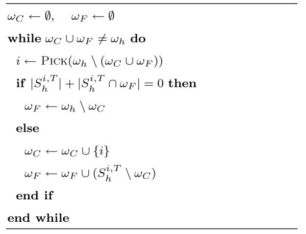
With those definitions a splitting into coarse and fine grid nodes can be achieved. For our application, a modified splitting algorithm is used [22, §4.6] as shown in Algorithm 2. Therein, the function

$$i\leftarrow \text{Pick}({\omega }_h\backslash ({\omega }_C\cup {\omega }_F\left)\right)$$

returns a node i for which the number $\mid S_h^{i,T}\mid +\mid S_h^{i,T}\cap {\omega }_F\mid$ is maximal. Note that tissue conductivity inhomogeneity and anisotropy are taken into account within the coarsening algorithm.

Algorithm 2.

$\text{COARSE}:\left(\right\{S_h^{i,T}\},{\omega }_h)\to ({\omega }_C,{\omega }_F)$

Prolongation

To achieve prolongation, the operator P_h,H : V_H ↦ V_h has to be defined correctly. The form that turned out to be the most efficient for the presented application was proposed in [14] and is given by

$$P_{h,H}^{\left[ij\right]}=\{\begin{array}{cc}1\hfill & i=j\in {\omega }_C,\hfill \\ 1∕\mid S_h^{i,T}\cap {\omega }_C\mid \hfill & i\in {\omega }_F,j\in S_h^{i,T}\cap {\omega }_C,\hfill \\ 0\hfill & \text{else}.\hfill \end{array}\phantom{\}}$$ (21)

After the proper definition of the prolongation and coarse grid operators, it is possible to create in a recursive way a matrix hierarchy and an associated multigrid cycle, shown in Algorithm 3. Therein, the variable COARSEGRID denotes the level at which a direct solver is applied. For an m-V (ν_F, ν_B)-cycle AMG preconditioned CG method, the operation SOLVE C_hw_h = r_h in Algorithm 1 is realized by m calls of MG(K_h,w_h, r_h, ν_F, ν_B). Specific performance optimizations for the AMG preconditioner used in this study are described in detail in [10, Section 2].

Algorithm 3.

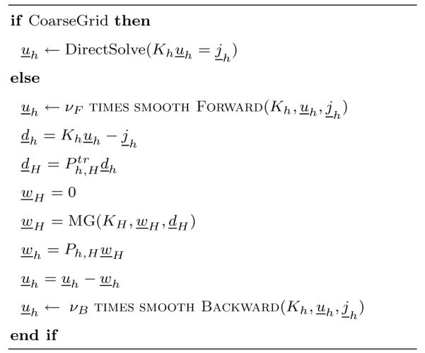
V-cycle MG : (K_h, u_h, j_h, ν_F, ν_B) → (u_h)

3. Methods

3.1. Validation platform

The numerical examinations of the theory presented above were carried out in a four-layer sphere model with anisotropic skull compartment whose parameterization is shown in Table 1. For the choice of these parameters, we closely followed [12,15]. Forward solutions were computed for dipoles of 1 nAm amplitude located on the y axis at depths of 0% to 98.7% (in 1 mm steps) of the brain compartment (78 mm radius) using both radial (directed away from the center of the model) and tangential (directed parallel to the scalp surface) dipole orientations. Eccentricity is defined here as the percent ratio of the distance between the source location and the model midpoint divided by the radius of the inner sphere (78 mm). The most eccentric source position considered was thus only 1 mm below the CSF compartment. To achieve error measures which were independent of the specific choice of the sensor configuration, we distributed 748 electrodes in a regular fashion over the outer sphere surface. All simulations ran on a Linux-PC with an Intel Pentium 4 processor (3.2GHz) using the SimBio software environment [31] in which the algebraic multigrid solver package PEBBLES was embedded [9,38,42,10].

Table 1.

Parameterization of the anisotropic four-layer sphere model.

Medium	Scalp	Skull	CSF	Brain
Outer shell radius	92mm	86mm	80mm	78mm
Tangential conductivity	0.33S/m	0.042S/m	1.79S/m	0.33S/m
Radial conductivity	0.33S/m	0.0042S/m	1.79S/m	0.33S/m

3.2. Analytical solution in an anisotropic multilayer sphere model

De Munck and Peters [5] derived series expansion formulas for a mathematical dipole in a multi-layer sphere model, denoted here as the analytical solution. The model consists of S shells with radii r_S < r_S−1 < … < r₁ and constant radial, ${\sigma }^{\mathrm{rad}}\left(r\right)={\sigma }_j^{\mathrm{rad}}\in {\mathbb{R}}^{+}$, and constant tangential conductivity, ${\sigma }^{\mathrm{tang}}\left(r\right)={\sigma }_j^{\mathrm{tang}}\in {\mathbb{R}}^{+}$, within each layer r_j+1 < r < r_j. It is assumed that the source at position x₀ with radial coordinate $r_0\in \mathbb{R}$ is in a more interior layer than the measurement electrode at position $x_e\in {\mathbb{R}}^3$ with radial coordinate $r_e=r_1\in \mathbb{R}$. The spherical harmonics expansion for the mathematical dipole (2) is expressed in terms of the gradient of the monopole potential to the source point. Using an asymptotic approximation and an addition-subtraction method to speed up the series convergence yields

$${\varphi }_{\mathrm{ana}}(x_0,x_e)=\frac{1}{4\pi }\langle \mathbf{M},S_0\frac{x_e}{r_e}+(S_1-\cos {\omega }_{0e}{S}_0)\frac{x_0}{r_0}\rangle$$

with ω_0e the angular distance between source and electrode, and with

$$S_0=\frac{F_0}{r_0}\frac{\Lambda }{{(1-2\Lambda \cos {\omega }_{0e}+{\Lambda }^2)}^{3∕2}}+\frac{1}{r_0}\sum _{n=1}^{\infty }\left\{\right(2n+1\left)R_n\right(r_0,r_e)-F_0{\Lambda }^n\}{P}_n^{\prime }\left(\cos {\omega }_{0e}\right)$$ (22)

and

$$S_1=F_1\frac{\Lambda \cos {\omega }_{0e}-{\Lambda }^2}{{(1-2\Lambda \cos {\omega }_{0e}+{\Lambda }^2)}^{3∕2}}+\sum _{n=1}^{\infty }\left\{\right(2n+1\left)R_n^{\prime }\right(r_0,r_e)-F_{1}n{\Lambda }^n\}{P}_n\left(\cos {\omega }_{0e}\right).$$ (23)

The coefficients R_n and their derivatives, $R_n^{\prime }$, are computed analytically and the derivative of the Legendre polynomials, P_n, are determined by means of a recursion formula. We refer to [5] for the derivation of the above series of differences and for the definition of F₀, F₁ and ʌ. Here, it is only important that the latter terms are independent of n and that they can be computed from the given radii and conductivities of layers between source and electrode and of the radial coordinate of the source. The computations of the series (22) and (23) are stopped after the k-th term if the following criterion is fulfilled

$$t_k∕t_0\le \upsilon ,t_k≔(2k+1)R_k^{\prime }-F_{1}k{\Lambda }^k.$$ (24)

In the following simulations, a value of 10⁻⁶ was chosen for ν in (24). Using the asymptotic expansion, no more than 30 terms were needed for the series computation at each electrode.

3.3. Tetrahedral mesh generation

The FE meshes of the four-layer sphere model were generated by the software TetGen [28] which used a Constrained Delaunay Tetrahedralization (CDT) approach [30,29]. This meshing procedure starts with the preparation of a suitable boundary discretization of the model in which for each of the layers and for a given triangle edge length, nodes are distributed in a regular fashion and connected through triangles. This yields a valid triangular surface mesh for each of the layers. Meshes of different layers are not intersecting each other. The CDT approach is then used to construct a tetrahedralization conforming to the surface meshes. It first builds a Delaunay tetrahedralization starting with the vertices of the surface meshes. The CDT then uses a local degeneracy removal algorithm combining vertex perturbation and vertex insertion to construct a new set of vertices which includes the input set of surface vertices. In a last step, a fast facet recovery algorithm is used to construct the CDT [30,29].

This approach is combined with two further constraints to the size and shape of the tetrahedra. The first constraint is important for the generation of quality tetrahedra. If R denotes the radius of the unique circumsphere of a tetrahedron and L its shortest edge length, the so-called radius-edge ratio of the tetrahedron can be defined as

$$\text{radius}-\text{edge}-\text{ratio}=R∕L.$$ (25)

The radius-edge ratio can distinguish almost all badly-shaped tetrahedra except one type of tetrahedra, so-called slivers. A sliver is a very flat tetrahedron which has no small edges, but can have arbitrarily large dihedral angles (close to π). For this reason, an additional mesh smoothing and optimization step is required to remove the slivers and improve the overall mesh quality.

A second constraint can be used to restrict the volume of the generated tetrahedra in a certain compartment. We follow the formula for regular tetrahedra:

$$\text{volume}=\sqrt{2}∕12\cdot {\text{edge}}^3$$ (26)

Table 2 shows the number of nodes and elements of the six tetrahedra models used for the solver run-time comparison and accuracy tests. factor indicates the ratio of the number of nodes of the most highly resolved to both other models within each group. Additionally, the table contains the chosen radius-edge-ratio (see Equation (25)), the average edge length of the four triangular surface meshes, the corresponding volume constraints (see Equation (26)) for the tetrahedra and the compartments where the volume constraint is not applied. The most highly resolved meshes tet503K and tet508K of both groups had approximately the same resolution, while the others were chosen to have a factor of 4 coarser resolution with regard to the number of nodes. The meshes of group 1 concentrated the nodes in the outer three compartments because no volume constraint was applied for the inner brain compartment, while the nodes in the meshes of group 2 were distributed in a regular way throughout all four compartments. The meshes of group 1 were thus preferentially beneficial to the full subtraction approach, since the entries of the volume integral in Equation (10) are zero ((σ(x)–σ₀) = 0 for all x in the brain compartment) so that a coarse resolution can be expected to have no impact on the overall numerical accuracy, but will reduce the computational cost. In contrast, the meshes of group 2 were beneficial to both direct potential approaches. Figure 1 shows samples from the six tetrahedra models that were generated using the parametrizations from Table 2.

Table 2.

The six tetrahedra models used for the solver time comparison and accuracy tests. The table shows the number of nodes and elements of each mesh and factor indicates the ratio of the number of nodes of the most highly resolved to both other models within each group. Additionally, the chosen radius-edge-ratio (see Equation (25)), the average edge length of the four triangular surface meshes, the corresponding volume constraint (see Equation (26)) and the compartments where the volume constraint was not applied are indicated.

	Group 1			Group 2
Model	tet503K	tet125K	tet33K	tet508K	tet128K	tet32K
nodes	503,180	124,624	32,509	508,435	127,847	31,627
elements	3,068,958	733,022	187,307	3,175,737	781,361	190,060
factor	1	4.04	15.48	1	3.98	16.08
radius-edge-ratio	1.0	1.0	1.1	1.0	1.0	1.1
edge (in mm)	1.75	2.7	5.2	2.42	3.9	6.87
volume (in mm3)	0.63	2.32	16.57	1.67	6.99	38.21
no volume constraint in	brain	brain	brain	/	/	/

Fig. 1.

Cross-sections of the six tetrahedral meshes of the four compartment sphere model. The corresponding parametrizations of the models are shown in Table 2. Visualization was done using the software TetView [28].

3.4. Error criteria

We compared numerical solutions with analytical solutions using three common error criteria [16,3,34,15,26]. The relative (Euclidean) error (RE) is defined as

$$\mathrm{RE}≔\frac{{\Vert {\underset{‒}{\varphi }}_{\mathrm{num}}-{\underset{‒}{\varphi }}_{\mathrm{ana}}\Vert }_2}{{\Vert {\underset{‒}{\varphi }}_{\mathrm{ana}}\Vert }_2},$$

where ${\underset{‒}{\varphi }}_{\mathrm{ana}}$, ${\underset{‒}{\varphi }}_{\mathrm{num}}\in {\mathbb{R}}^{\mathrm{m}}$ denote the analytical and the numerical solution vectors, respectively, at the m = 748 measurement electrodes. We furthermore defined

$$\mathrm{RE}(\%)≔100\cdot \mathrm{RE},\max \mathrm{RE}(\%)≔\underset{j}{\max }\left(\mathrm{RE}{(\%)}_j\right)$$ (27)

where j is the source eccentricity. In order to better distinguish between the topography (driven primarily by changes in dipole location and orientation) and the magnitude error (indicating changes in source strength), Meijs et al. [16] introduced the relative difference measure (RDM) and the magnification factor (MAG), respectively. For the RDM, we can show that

$$\mathrm{RDM}≔{\Vert \frac{1}{{\Vert {\underset{‒}{\varphi }}_{\mathrm{ana}}\Vert }_2}{\underset{‒}{\varphi }}_{\mathrm{ana}}-\frac{1}{{\Vert {\underset{‒}{\varphi }}_{\mathrm{num}}\Vert }_2}{\underset{‒}{\varphi }}_{\mathrm{num}}\Vert }_2=\sqrt{2\left(1-\cos \angle ({\underset{‒}{\varphi }}_{\mathrm{ana}},{\underset{‒}{\varphi }}_{\mathrm{num}})\right)}.$$ (28)

It therefore holds that 0 ≤ RDM ≤ 2, so that we can furthermore define

$$\mathrm{RDM}(\%)≔100\cdot \mathrm{RDM}∕2,\max \mathrm{RDM}(\%)≔\underset{j}{\max }\left(\mathrm{RDM}{(\%)}_j\right).$$ (29)

The MAG is defined as

$$\mathrm{MAG}≔{\Vert {\underset{‒}{\varphi }}_{\mathrm{num}}\Vert }_2∕{\Vert {\underset{‒}{\varphi }}_{\mathrm{ana}}\Vert }_2$$

so that error minimum is at MAG = 1 and we therefore defined

$$\mathrm{MAG}(\%)=\mid 1-\mathrm{MAG}\mid \cdot 100,\max \mathrm{MAG}(\%)≔\underset{j}{\max }\left(\mathrm{MAG}{(\%)}_j\right).$$ (30)

With maxRE(%)^k we denote the maximal relative error in percent over all source eccentricities for an accuracy level of ACCURACY = 10^−k. The so-called plateau-entry for an iterative solver is then defined as the first k at which the condition

$$\mid \max \mathrm{RE}{(\%)}^k-\max \mathrm{RE}{(\%)}^{k+1}\mid ∕\max \mathrm{RE}{(\%)}^{k+1}<0.05$$ (31)

is true.

3.5. FEM and solver parameter settings

The parameters of the Venant approach were chosen as proposed in [4]: The maximal dipole order (n₀ in [4, Equation (22)]) and the scaling reference length (α_ref in [4, Equation (23)]) were set to n₀ = 2 and α_ref = 20.0 mm, respectively. Since the chosen mesh size was a large factor smaller than the reference length, the second order term ${\left(\right(\Delta {\stackrel{‒}{x}}_{ki}^r)}^2$ in [4, Equation (23)]) was small and the model focused on fulfilling the dipole moments of the zeros and first order. The exponent of the source weighting matrix (n_s in [4, Equation (25)]) was fixed to n_s = 1 and the regularization parameter (λ_D in [4, Equation (25)]) was chosen as λ_D = 10⁻⁶. These settings effect a spatial concentration of the monopole loads in the dipole axis around the dipole location.

The initial solution guess for all solvers was a zero potential vector. For the IC(0), ς = 0 was chosen for (14). For the AMG-CG, the 1-V (1, 1)-cycle AMG-preconditioner was used with α = 0.01 for (20). The factorization in Algorithm 3 was carried out whenever the size of the coarsest grid (COARSEGRID) in the preconditioner-setup was below 1000 and the coarse system was solved using a Cholesky-factorization. The setup times for the preconditioners were neglected in all calculations of computational cost because this step must be performed only once per head model. The evaluation with regard to relative solver accuracy in Algorithm 1 was limited to the discrete set of accuracy levels ACCURACY = 10^−k with k ∈ {0, … , 9}.

4. Results

4.1. Numerical error versus potential approach

In a first study, we compared the numerical accuracy of the full subtraction approach (Section 2.1.1) with the two direct methods: Venant (Section 2.1.3) and partial integration (Section 2.1.2). Figure 2 shows the RE(%) for the different source eccentricities for the two finest models tet503K of group 1 (left) and tet508K of group 2 (right) (see Figure 1 and Table 2) with regard to the full subtraction (top row), the Venant (middle row) and the partial integration approach (bottom row). The results were computed with the AMG-CG and the necessary ACCURACY in Algorithm 1 for the plateau-entry (31) is indicated for both source orientation scenarios. In Figure 3, the maximal RE, RDM and MAG errors over all source eccentricities at the AMG-CG plateau-entry (31) are shown for all tetrahedra models, both source orientation scenarios and the three dipole modeling approaches.

Fig. 2.

RE(%) versus source eccentricity for the two most highly resolved models tet503K of group 1 (left) and tet508K of group 2 (right) using the full subtraction (top row), the Venant (middle row) and the partial integration (bottom row) potential approaches. The necessary ACCURACY in Algorithm 1 for the plateau-entry (31) of the AMG-CG is indicated for both source orientation scenarios. Note that the y-axis is differently scaled.

Fig. 3.

maxRE(%), maxRDM(%) and maxMAG(%) accuracies for the full subtraction, the Venant and the partial integration approach for all six tetrahedra models (see Figure 1 and Table 2) and both tangential (left) and radial (right) source orientation scenarios at the AMG-CG plateau-entry (31).

Figure 2 clearly presents the advantages of the full subtraction approach whose error curves are smooth, while Venant and partial integration show an oscillating behavior. With RDM and MAG errors below 1% over all source eccentricities and for both orientation scenarios (see Figure 3), the full subtraction approach performs best for all source eccentricities for model tet503K (its mesh resolution was sufficiently high and the FE nodes were concentrated in the compartments CSF, skull and skin), where both direct approaches showed oscillations with a relatively high magnitude. As the results for model tet508K show, the oscillation magnitudes for the direct approaches could be strongly reduced by means of distributing the FE nodes in a regular way over all four compartments, hence decreasing the mesh size in the brain compartment. Nevertheless, even for model tet508K, the full subtraction approach was the most accurate method for nearly all source eccentricities. It was only outperformed by partial integration for the source which was only 1 mm below the CSF compartment. As both Figures 2 and 3 show, the partial integration approach performed well if the mesh was sufficiently fine in the brain compartment. The oscillation magnitudes of the Venant approach were generally even slightly smaller than for the partial integration approach, with only one exception (the result for the radial source 1 mm below the CSF compartment, shown in the middle row of Figure 2). The main reason for the outlier was that for the source 1 mm below the CSF, monopoles were positioned in the CSF compartment, which had a strong effect on the MAG for the radially oriented source.

4.2. Numerical error versus PCG accuracy

Figure 4 shows the numerical error maxRE(%) versus the PCG solver ACCURACY from Algorithm 1 for the discrete set of accuracy levels from 10⁰ to 10⁻⁹. Results for the high-resolution model tet503K of group 1 are shown in the left and from the high-resolution model tet508K of group 2 in the right column for the AMG-CG (top row), the IC(0)-CG (middle row) and the Jacobi-CG (bottom row).

Fig. 4.

maxRE(%) versus PCG solver ACCURACY (see Algorithm 1 and Section 3.5) for models tet503K of group 1 (left column) and tet508K of group 2 (right column) for the AMG-CG (top row), the IC(0)-CG (middle row) and the Jacobi-CG (bottom row). Source orientations and potential approaches can be distinguished by their specific labels. The plot is in log-log scale.

The PCG accuracy measures the error in the solution vector of the FE linear equation system (8) (correction potential), (11) and (13) (total potential). For the full subtraction approach, maxRE(%) was thus not equal to 100 for ACCURACY = 10⁰ because ${\underset{‒}{\varphi }}_{\mathrm{num}}$ is equal to the analytically computed singularity potential ${\underset{‒}{\Phi }}_0$ from Equation (5). Because the PCG accuracy is measured in the $K_h{C}_h^{-1}{K}_h\text{-energy}$ norm, the plateau-entry (31) differs for different preconditioners C_h. As shown in Figure 4 for the high-resolution models and as collected in Table 3 for all six tetrahedra models, the maximally needed k (for a PCG accuracy of ACCURACY = 10^−k) decreased when the preconditioning quality increased (except for the radial source orientation in model tet503K, see Fig. 4). Furthermore, as Table 3 shows, a higher PCG accuracy was needed for the plateau-entry when the mesh resolution increased.

Table 3.

Maximally needed k ∈ {0, … , 9} for a PCG ACCURACY = 10^−k for the plateau-entry (31) over all three potential approaches.

Group 1
	tangential source			radial source
solver	AMG-CG	IC(0)-CG	Jacobi-CG	AMG-CG	IC(0)-CG	Jacobi-CG
tet503K	5	6	7	6	5	6
tet125K	5	5	6	5	5	6
tete33K	4	5	6	3	3	5

Group 2
	tangential source			radial source
solver	AMG-CG	IC(0)-CG	Jacobi-CG	AMG-CG	IC(0)-CG	Jacobi-CG
tet508K	6	6	7	6	7	8
tet128K	4	5	6	4	4	6
tete32K	3	5	6	3	4	5

4.3. Numerical error versus solver time

In a last study, we compared solver wall-clock time versus numerical accuracy for the three different CG preconditioners AMG, IC(0) and Jacobi.

The average setup time for the AMG- and the IC(0)-preconditioner is given in Table 4. In the following, the time for the setup of the preconditioner was not included, because this step was carried out only once per head model.

Table 4.

Average setup time (sec.) for the AMG- and the IC(0)-preconditioner.

	group 1			group 2
preconditioner	tet503K	tet125K	tet33K	tet508K	tet128K	tet32K
AMG	17.84	4.58	1.37	15.95	3.29	0.72
IC(0)	0.95	0.20	0.04	0.84	0.19	0.04

In Figure 5, the solver time is shown versus the maxRE(%) for different levels of PCG accuracy for models tet503K and tet33K of group 1. The largest examined PCG ACCURACY level 10^−k is indicated in the figure. Please note that this level does not necessarily correspond to the plateau-entry level. In most cases results are presented up to one level higher.

Fig. 5.

Solver time versus maxRE(%) for models tet503K and tet33K of group 1 for tangentially and radially oriented sources for the potential approaches full subtraction (left), Venant (middle), and partial integration (right). Results are presented for the three different CG preconditioners AMG, IC(0) and Jacobi. Each marker represents a PCG ACCURACY = 10^−k level and the largest examined level is indicated. The x-axis is in log scale.

For all tetrahedra models of groups 1 and 2, average solver times and iteration counts over all source eccentricities, source orientations and potential approaches for a plateau-entry (31) are collected in Table 5. Both Figure 5 and Table 5 clearly show the superiority of the AMG preconditioner. In all cases, even for the low-resolution grids tet33K and tet32K, the AMG-CG was the fastest solver, followed by the IC(0)-CG and the Jacobi-CG. The main result of Table 5 is the so-called gain factor, which is defined here as the result (solver time or iteration count) for the Jacobi-CG divided by the result for the AMG-CG. The gain factors clearly showed that the higher the mesh-resolution, i.e., the higher the condition number of the corresponding FE stiffness matrix, the larger the difference in performance between AMG-CG, IC(0)-CG, and Jacobi-CG. An increasing mesh-resolution led to a strong increase in the number of iterations of IC(0)-CG (factor of 3.2 between tet503K and tet33K and 4.1 between tet508K and tet32K) and Jacobi-CG (factor of 3.0 between tet503K and tet33K and 3.6 between tet508K and tet32K), while the number of AMG-CG iterations was only slightly increasing (factor of 1.9 between tet503K and tet33K and 1.8 between tet508K and tet32K). This clearly shows the stronger h-dependence of the IC(0) and Jacobi preconditioners.

Table 5.

Average solver time (sec.) and iteration count (iter) over all source eccentricities, source orientations and potential approaches for plateau-entry (31). For all tetrahedra models of groups 1 and 2, results are presented for the three different CG preconditioners AMG, IC(0) and Jacobi. The gain factor indicates the performance gain of the AMG-CG relative to the Jakobi-CG.

	group 1						group 2
	tet503K		tet125K		tet33K		tet508K		tet128K		tet32K
solver	time	iter	time	iter	time	iter	time	iter	time	iter	time	iter
AMG-CG	12.25	11.20	1.87	9.04	0.18	5.89	9.18	10.40	1.36	7.27	0.15	5.81
IC(0)-CG	112.03	233.43	8.40	128.39	0.45	72.63	72.41	215.05	5.20	98.96	0.31	52.84
Jacobi-CG	167.82	679.43	16.98	414.00	0.76	229.52	99.60	578.04	9.62	331.15	0.47	161.68
gain factor	13.70	60.66	9.08	45.8	4.22	38.97	10.85	55.58	7.07	45.55	3.13	27.83

5. Discussion

The goals of this technical study of finite element (FE) based solution techniques for the electroencephalographic forward problem were twofold. The first aim was to compare three efficient iterative FE solver techniques under realistic conditions that still allowed quasi-analytical solutions. The second aim was to evaluate three different numerical formulations of the current dipole, which is the bioelectric source most commonly used to represent neural electrical activity. A major motivation of such studies is the special need to achieve high accuracy and efficiency with FE based approaches for this problem. The many advantages of this approach are often hindered by the unacceptable computation costs of implementing it so that improved efficiency will provide substantial progress to the field.

When using the $K_h{C}_h^{-1}{K}_h\text{-energy}$ norm stopping criterion for the PCG algorithm applied on meshes with up to 500K nodes, a relative solver accuracy of 10⁻⁶ for AMG-CG, 10⁻⁷ for IC(0)-CG and 10⁻⁸ for Jacobi-CG was necessary and sufficient to fall below the discretization error. The AMG-CG achieved an order of magnitude higher computational speed than the CG with the standard preconditioners with an increasing gain factor with decreasing mesh size. The increasing gain factor shows that the convergence rate of the Jacobi- and IC(0)-preconditioning methods are much more dependent on the mesh size h than the AMG-CG, as discussed in detail in Section 2.2.3. However, while for the geometric multigrid, an h-independent convergence rate and an h-independent condition number can be proven ([11, Lemma 10.7.1,Theorem 10.7.15]), the AMG-CG was not optimal in our application with a slight h-dependence shown by a slightly increasing iteration count with increasing mesh resolution. Such a result had to be expected because the source analysis stiffness matrix was not an M-matrix and the prolongation operator of the presented AMG-CG was tuned for speed and not for an optimal behavior with regard to the iteration count. A discrete harmonic extension as proposed in [22] improved the interpolation properties, but the application of this prolongation operator is more expensive, which decreased the overall run-time performance in our application.

We generated two groups of Constrained Delaunay tetrahedralization (CDT) FE meshes [30,29], tuned for the specific needs of the different potential approaches. In group 1, for the full subtraction approach [7], FE nodes were concentrated in the CSF, skull and skin, while the brain compartment was meshed as coarsely as possible. Group 2 was tuned for the needs of both direct potential approaches [45,4,1,37], which profit more from a regular distribution of FE nodes over all four compartments and especially a higher resolution at the source positions.

With regard to the numerical error, in the tuned FE meshes with about 500K nodes we achieved high accuracies—in the range of a few percent maximal relative error (maxRE)—over all source eccentricities for both the full subtraction and the two direct potential approaches. With a maximal relative difference measure (maxRDM) and a maximal magnification factor (maxMAG) of less than 1% over all source eccentricities for sources up to 1 mm below the CSF compartment (model tet503K, maximal examined eccentricity of 98.7%), the full subtraction approach performed consistently better than both direct approaches. We found that the instability of the full subtraction approach with regard to the RE for high source eccentricities was mainly a magnitude instability (MAG), not a topographic one (RDM). Our results clearly illustrate the advantages of the full subtraction approach as long as the homogeneity condition is sufficiently fulfilled, i.e., as long as the distance of the source to the next conductivity inhomogeneity is large enough or the resolution of the FE mesh at the nearest conductivity inhomogeneity to the source is fine enough. A theoretical reasoning for this finding is given in [39]. While error curves oscillated for both direct approaches, they were smooth for the full subtraction approach as long as the homogeneity condition was sufficiently fulfilled. The smoothness can be explained by the fact that the singularity potential is sensitively modeling the details of the point dipole source singularity while the FE method is able to accurately model the smooth correction potential. The oscillating behavior of the direct approaches can easily be understood for the partial integration approach. Since linear basis functions were used, the right-hand side vector (12) and thus the computed solution for the total potential in (11) is constant over any finite element for all sources with moment M₀ and any location x₀ within the finite element. For partial integration with linear basis functions, the inverse source localization resolution is thus bounded by the size of the element, which should be fine as long as high-resolution FE meshes are used. The direct approach oscillations should therefore not necessarily be a problem with regard to the inverse problem. It has furthermore been shown using quasi-analytically computed reference potentials in a four-layer anisotropic sphere model and single dipole fit reconstructions based on the Venant FE approach in a regular tetrahedral FE mesh with 161K nodes, that localization errors were in the 1 millimeter range [40] and might thus most often be neglected when compared to errors due to, e.g., EEG data noise, inaccurate tissue segmentation and conductivity modeling.

Schimpf et al. [26] investigated different FE potential approaches in a four-layer sphere model with isotropic skull and sources up to 1 mm below the CSF compartment. In their report, a regular 1 mm cube model was used (thus a much higher FE resolution) and a maxRDM of 7% and a maxMAG of 25% was achieved with a subtraction approach, which performed best in their comparison. Awada et al. [1] implemented a two-dimensional subtraction approach and compared its numerical accuracy with a partial integration method in a two-dimensional multi-layer sphere model. A direct comparison with our results is therefore difficult, but the authors concluded that the subtraction method was more accurate than the partial integration direct approach. In a locally refined (around the source singularity) tetrahedral mesh with 12,500 nodes of a four-layer sphere model with anisotropic skull and first order FE basis functions in a subtraction approach, Bertrand et al. [3] reported a maxRDM of above 20% and a maxMAG up to 70% for a maximal eccentricity of 97.6%. Van den Broek [34] used a subtraction approach in a locally refined (around the source singularity) tetrahedral mesh with 3,073 nodes of a three-layer sphere model with anisotropic skull. For the maximal examined eccentricity of 94.2%, they reported a maxRDM of up to 50%.

However, the right-hand side (RHS) vector is expensive to compute and is densely populated (i.e., N_h non-zeros) for the full subtraction approach (10) and sparse with just some few (|NODESOFELE| for partial integration (12), and C for Venant (13)) non-zero vector entries for the direct approaches, which has implications for the computational effort when using the fast FE transfer matrix approach for EEG and MEG [43] (additionally, see [37,8,12]), which limits the total number of FE linear equation systems to be solved for any inverse method to the number of sensors m. After solving m FE linear equation systems to compute the transfer matrix, each forward problem can be solved by a single multiplication of the RHS vector with the transfer matrix [43], resulting in a computational effort of 2 * m * P operations with P = N_h for the full subtraction, P = |NODESOFELE| for partial integration and P = C for the Venant approach. Note that the transfer matrix approach can not be used if the mesh is adapted according to varying source positions within the inverse problem. We therefore attempted to avoid local mesh refinement techniques as used in [3,34].

The following limitations of the presented work are important and can be seen as an outlook for our future studies. Oscillations of the direct potential approaches might be avoided. For example, the use of higher order basis functions might cure the oscillation problem for the partial integration approach. For both examined direct methods, the oscillations might be avoided by means of precomputing a lead field (i.e., many forward solutions) for those source positions with minimal errors (e.g., only at the barycenters of brain finite elements for the partial integration approach and only at brain FE nodes for the Venant approach) and consequently using a lead field interpolation technique [46] for all other forward solutions. Lead field extrapolation [46] has to be examined as a concept to further decrease the numerical error for eccentric sources. Such an approach might be particularly fruitful for the subtraction method, where a violation of the homogeneity condition led to especially large numerical errors or instabilities as shown in Figure 2 for the most eccentric source in especially the model tet508K of group 2. In our study, we examined numerical errors for a single source at each discrete 1mm step eccentricity level through the inner compartment along the y axis. By means of the error oscillations and magnitudes for the direct methods and the specific sensitivity of the subtraction method for eccentric sources, the dependence of all three dipole modeling approaches on the specific FE mesh properties has been shown. A further important measure for establishing the validity of the presented results would be a more statistical error measure where, for each eccentricity level, not only the error of a single source on the y axis is evaluated, but an error statistic is evaluated over many sources with different positions in the volume conductor and/or sources with slightly varying (e.g., 0.1 mm) source positions around each eccentricity level.

6. Conclusion

The AMG-CG turned out to achieve an order of magnitude higher computational speed than Jacobi-CG or incomplete Cholesky-CG for the FEM based EEG forward and inverse problem. Our results corroborate the theoretical results that the higher the FE resolution, the greater the advantage of using MG preconditioning. The AMG-CG together with the fast transfer matrix approach now enable resolutions which seemed to be impracticable before. In the comparison of dipole modeling approaches, highest accuracies were achieved with the full subtraction approach in CDT meshes where nodes were concentrated in the compartments CSF, skull and skin. However, the accuracy of the subtraction approach is especially dependent on a sufficiently fulfilled homogeneity condition, so that the direct potential approaches partial integration and Venant, which also performed well in our comparison, might be even more appropriate if white matter conductivity anisotropy is taken into account.

References

- [1].Awada K, Jackson D, Williams J, Wilton D, Baumann S, Papanicolaou A. Computational aspects of finite element modeling in EEG source localization. IEEE Trans Biomed. Eng. 1997;44(8):736–751. doi: 10.1109/10.605431. [DOI] [PubMed] [Google Scholar]
- [2].Baillet S, Mosher J, Leahy R. Electromagnetic brain mapping. IEEE Signal Processing Magazine. 2001 November;18(6):14–30. [Google Scholar]
- [3].Bertrand O, Thévenet M, Perrin F. 3D finite element method in brain electrical activity studies. In: Nenonen J, Rajala H, Katila T, editors. Biomagnetic Localization and 3D Modelling. 1991. Report of the Dep. of Tech.Physics, Helsinki University of Technology. [Google Scholar]
- [4].Buchner H, Knoll G, Fuchs M, Rienäcker A, Beckmann R, Wagner M, Silny J, Pesch J. Inverse localization of electric dipole current sources in finite element models of the human head. Electroenc. Clin. Neurophysiol. 1997;102:267–278. doi: 10.1016/s0013-4694(96)95698-9. [DOI] [PubMed] [Google Scholar]
- [5].de Munck J, Peters M. A fast method to compute the potential in the multi sphere model. IEEE Trans Biomed. Eng. 1993;40(11):1166–1174. doi: 10.1109/10.245635. [DOI] [PubMed] [Google Scholar]
- [6].de Munck J, van Dijk B, Spekreijse H. Mathematical dipoles are adequate to describe realistic generators of human brain activity. IEEE Trans Biomed. Eng. 1988;35(11):960–966. doi: 10.1109/10.8677. [DOI] [PubMed] [Google Scholar]
- [7].Drechsler F, Wolters C, Dierkes T, Si H, Grasedyck L. A highly accurate full subtraction approach for dipole modelling in EEG source analysis using the finite element method. Max-Planck-Institut für Mathematik in den Naturwissenschaften; 2007. Techn. Report 95. http://www.mis.mpg.de/publications/preprints/2007/prepr2007-95.html. [Google Scholar]
- [8].Gencer N, Acar C. Sensitivity of EEG and MEG measurements to tissue conductivity. Phys.Med.Biol. 2004;49:701–717. doi: 10.1088/0031-9155/49/5/004. [DOI] [PubMed] [Google Scholar]
- [9].Haase G, Kuhn M, Reitzinger S. Parallel AMG on distributed memory computers. SIAM J. Sci.Comp. 2002;24(2):410–427. [Google Scholar]
- [10].Haase G, Reitzinger S. Cache issues of algebraic multigrid methods for linear systems with multiple right-hand sides. SIAM J. Sci.Comp. 2005;27(1):1–18. [Google Scholar]
- [11].Hackbusch W. Iterative solution of large sparse systems of equations, Springer Verlag. Applied Mathematical Sciences. 1994;95 [Google Scholar]
- [12].Hallez H, Vanrumste B, Hese PV, D’Asseler Y, Lemahieu I, de Walle RV. A finite difference method with reciprocity used to incorporate anisotropy in electroencephalogram dipole source localization. Phys.Med.Biol. 2005;50:3787–3806. doi: 10.1088/0031-9155/50/16/009. [DOI] [PubMed] [Google Scholar]
- [13].Jung M, Langer U. Applications of multilevel methods to practical problems. Surv.Math.Ind. 1991;1:217–257. [Google Scholar]
- [14].Kickinger F. Algebraic multigrid for discrete elliptic second-order problems. In: Hackbusch W, editor. Multigrid Methods V. Proceedings of the 5th European Multigrid conference; Berlin. Springer; 1998. [Google Scholar]
- [15].Marin G, Guerin C, Baillet S, Garnero L, Meunier G. Influence of skull anisotropy for the forward and inverse problem in EEG: simulation studies using the FEM on realistic head models. Human Brain Mapping. 1998;6:250–269. doi: 10.1002/(SICI)1097-0193(1998)6:4<250::AID-HBM5>3.0.CO;2-2. [DOI] [PMC free article] [PubMed] [Google Scholar]
- [16].Meijs J, Weier O, Peters M, van Oosterom A. On the numerical accuracy of the boundary element method. IEEE Trans Biomed. Eng. 1989;36:1038–1049. doi: 10.1109/10.40805. [DOI] [PubMed] [Google Scholar]
- [17].Mohr M. Simulation of Bioelectric Fields: The Forward and Inverse Problem of Electroencephalographic Source Analysis. vol. Band 37 of Arbeitsberichte des Instituts für Informatik. Friedrich-Alexander-Universität Erlangen-Nürnberg; 2004. iSSN 1611-4205. [Google Scholar]
- [18].Murakami S, Okada Y. Contributions of principal neocortical neurons to magnetoencephalography and electroencephalography signals. J.Physiol. 2006;575(3):925–936. doi: 10.1113/jphysiol.2006.105379. [DOI] [PMC free article] [PubMed] [Google Scholar]
- [19].Ollikainen J, Vauhkonen M, Karjalainen P, Kaipio J. Effects of local skull inhomogeneities on EEG source estimation. Med.Eng.Phys. 1999;21:143–154. doi: 10.1016/s1350-4533(99)00038-7. [DOI] [PubMed] [Google Scholar]
- [20].Plonsey R, Heppner D. Considerations on quasi-stationarity in electro-physiological systems. Bull.Math.Biophys. 1967;29:657–664. doi: 10.1007/BF02476917. [DOI] [PubMed] [Google Scholar]
- [21].Reitzinger S. Ph.D. thesis. Schriften der Johannes-Kepler-Universität Linz, Reihe C - Technik und Naturwissenschaften; 2001. Algebraic multigrid methods for large scale finite element equations. No.36. [Google Scholar]
- [22].Ruge J, Stüben K. Algebraic multigrid (AMG) In: McCormick S, editor. Multigrid Methods. vol. 5 of Frontiers in Applied Mathematics. SIAM; Philadelphia: 1986. pp. 73–130. [Google Scholar]
- [23].Rullmann M, Anwander A, Dannhauer M, Warfield S, Duffy F, Wolters C. EEG source analysis of epileptiform activity using a 1mm anisotropic hexahedra finite element head model. NeuroImage. 2009;44(2):399–410. doi: 10.1016/j.neuroimage.2008.09.009. http://dx.doi.org/10.1016/j.neuroimage.2008.09.009. [DOI] [PMC free article] [PubMed] [Google Scholar]
- [24].Saad Y. Iterative methods for sparse linear systems. PWS Publishing Company; 1996. [Google Scholar]
- [25].Sarvas J. Basic mathematical and electromagnetic concepts of the biomagnetic inverse problem. Phys.Med.Biol. 1987;32(1):11–22. doi: 10.1088/0031-9155/32/1/004. [DOI] [PubMed] [Google Scholar]
- [26].Schimpf P, Ramon C, Haueisen J. Dipole models for the EEG and MEG. IEEE Trans Biomed. Eng. 2002;49(5):409–418. doi: 10.1109/10.995679. [DOI] [PubMed] [Google Scholar]
- [27].Schwarz H. Methode der finiten Elemente. B.G.Teubner Stuttgart; 1991. [Google Scholar]
- [28].Si H. TetGen, a quality tetrahedral mesh generator and three-dimensional delaunay triangulator, v1.3, user’s manual. Weierstrass Institute for Applied Analysis and Stochastics; 2004. Tech. Rep. 9. [Google Scholar]
- [29].Si H. Adaptive tetrahedral mesh generation by constrained Delaunay refinement. International Journal for Numerical Methods in Engineering. 2008;75(7):856–880. [Google Scholar]
- [30].Si H, Gärtner K. Meshing piecewise linear complexes by constrained Delaunay tetrahedralizations. Proc. 14th International Meshing Roundtable; Sandia National Laboratories; 2005. [Google Scholar]
- [31].SimBio -IPM and -NeuroFEM: Algorithms for inverse EEG and MEG source analysis. 2000 ( http://www.simbio.de) https://www.mrt.uni-jena.de/neurofem/index.php/Main_Page. since.
- [32].Stüben K. A review of algebraic multigrid. 1999 Nov. Techn. Report 69, GMD, http://www.gmd.de.
- [33].Tanzer O, Järvenpää S, Nenonen J, Somersalo E. Representation of bioelectric current sources using whitney elements in finite element method. Phys.Med.Biol. 2005;50:3023–3039. doi: 10.1088/0031-9155/50/13/004. [DOI] [PubMed] [Google Scholar]
- [34].van den Broek S. Ph.D. thesis. Proefschrift Universiteit Twente Enschede; The Netherlands: 1997. Volume conduction effects in EEG and MEG. [Google Scholar]
- [35].Waberski T, Buchner H, Lehnertz K, Hufnagel A, Fuchs M, Beckmann R, Rienäcker A. The properties of source localization of epileptiform activity using advanced headmodelling and source reconstruction. Brain Top. 1998;10(4):283–290. doi: 10.1023/a:1022275024069. [DOI] [PubMed] [Google Scholar]
- [36].Weinstein D, Zhukov L, Johnson C. Lead-field bases for EEG source imaging. Annals of Biomed. Eng. 2000;28(9):1059–66. doi: 10.1114/1.1310220. [DOI] [PubMed] [Google Scholar]
- [37].Weinstein D, Zhukov L, Johnson C. Lead-field bases for electroencephalography source imaging. Annals of Biomed.Eng. 2000;28(9):1059–1066. doi: 10.1114/1.1310220. [DOI] [PubMed] [Google Scholar]
- [38].Wolters C. Influence of Tissue Conductivity Inhomogeneity and Anisotropy on EEG/MEG based Source Localization in the Human Brain. Leipzig: 2003. (No. 39 in MPI Series in Cognitive Neuroscience, MPI of Cognitive Neuroscience Leipzig). iSBN 3-936816-11-5 (also: Univ., Diss., http://lips.informatik.uni-leipzig.de/pub/2003-33/en) [Google Scholar]
- [39].Wolters C, Köstler H, Möller C, Härtlein J, Grasedyck L, Hackbusch W. Numerical mathematics of the subtraction method for the modeling of a current dipole in EEG source reconstruction using finite element head models. SIAM J. on Scientific Computing. 2007;30(1):24–45. [Google Scholar]
- [40].Wolters CH. Habilitation in Mathematics, Faculty of Mathematics and Natural Sciences. University of Münster; Germany: 2008. Finite element method based electro- and magnetoencephalography source analysis in the human brain. [Google Scholar]
- [41].Wolters CH, Anwander A, Berti G, Hartmann U. Geometry-adapted hexahedral meshes improve accuracy of finite element method based EEG source analysis. IEEE Trans.Biomed.Eng. 2007;54(8):1446–1453. doi: 10.1109/TBME.2007.890736. [DOI] [PubMed] [Google Scholar]
- [42].Wolters CH, Anwander A, Reitzinger S, Haase G, Halgren E, Ahlfors S, Hämäläinen M, Cohen D. Algebraic multigrid with multiple right-hand-side treatment for an efficient computation of EEG and MEG lead field bases. BIOMAG2004, Proc. of the 14th Int. Conf. on Biomagnetism; Boston, USA. Aug.8-12,, 2004; http://www.biomag2004.org. [Google Scholar]
- [43].Wolters CH, Grasedyck L, Hackbusch W. Efficient computation of lead field bases and influence matrix for the FEM-based EEG and MEG inverse problem. Inverse Problems. 2004;20(4):1099–1116. [Google Scholar]
- [44].Wolters CH, Köstler H, Möller C, Härdtlein J, Anwander A. Numerical approaches for dipole modeling in finite element method based source analysis. International Congress Series 1300; June 2007; pp. 189–192. iSBN-13:978-0-444-52885-8, http://dx.doi.org/10.1016/j.ics.2007.02.014. [Google Scholar]
- [45].Yan Y, Nunez P, Hart R. Finite-element model of the human head: Scalp potentials due to dipole sources. Med.Biol.Eng.Comput. 1991;29:475–481. doi: 10.1007/BF02442317. [DOI] [PubMed] [Google Scholar]
- [46].Yvert B, Crouzeix-Cheylus A, Pernier J. Fast realistic modeling in bioelectromagnetism using lead-field interpolation. Human Brain Mapping. 2001;14:48–63. doi: 10.1002/hbm.1041. [DOI] [PMC free article] [PubMed] [Google Scholar]