

Abstract
A panel of cell lines of diverse molecular background offers an improved model system for high-content screening, comparative analysis, and cell systems biology. A computational pipeline has been developed to collect images from cell-based assays, segment individual cells and colonies, represent segmented objects in a multidimensional space, and cluster them for identifying distinct subpopulations. While each segmentation strategy can vary for different imaging assays, representation and subpopulation analysis share a common thread. Application of this pipeline to a library of 41 breast cancer cell lines is demonstrated. These cell lines are grown in 2D and imaged through immunofluorescence microscopy. Subpopulations in this panel are identified and shown to correlate with previous subtyping literature that was derived from transcript data.
1. INTRODUCTION
An emerging trend in high-content screening has been to use a panel of cell lines for evaluating therapeutic responses. The panel introduces the necessary molecular diversity to collect and analyze heterogeneous responses that lead to subpopulation identification. While the current method for subtyping has been limited to transcriptome data [1], we introduce a method to identify potential subpopulations through morphological and localization properties. The main advantage of the cell-based assays is in a large number of readouts, where every individual cell can be considered a single sensor responding to the environmental perturbation. These readouts embed biological and technical variations on a single cell basis in context. The main disadvantage is the absence of multiple molecular readouts. However, from a computational perspective, a number of challenges have to be addressed, i.e., segmentation, representation, and identifying subpopulations. The method is applied to a data set derived from a panel of breast cancer cell lines. Forty-one different breast cancer cell lines are grown in 2D, stained for nuclear and proliferation state, and imaged through florescence microscopy.
We have developed a computational pipeline that quantifies cellular morphology through segmentation and multidimensional representations. Subsequently, this representation enables the identification of subpopulations among all cell lines. The pipeline consists of three major steps: (i) segmentation, (ii) morphological feature extraction, and (iii) consensus clustering of morphological features.
2. MULTIDIMENSIONAL PROFILING OF CELLULAR MORPHOLOGIES
The first step in multivariate profiling is segmentation, which separates individual nuclei from their background, and decomposes touching nuclei. Segmentation enables multivariate profiling and subsequent subtyping.
2.1. Nuclear segmentation
In a typical 2D cell culture assay that is stained for nuclear compartment, some nuclei are isolated and others are clustered together to form clumps. As a part of our operational base, we have developed a system that first detects isolated nuclei, and then decomposes a clump of nuclei based on convexity analysis [2]. This system has recently been improved with a significantly better computational profile, and is being integrated into our high-content screening platform [3]. In this implementation, segmentation of nuclear regions is realized by detecting elliptic features [4] corresponding to potential bright regions. These regions are further filtered for their intensities and morphological features.
Let the linear scale-space representation of the original image I0(x, y) at scale σ be given by:
| (1) |
where G(x, y; σ) is the Gaussian kernel with a standard deviation of σ. For simplicity, I(x, y; σ) is also denoted as I(x, y) below. At each point (x, y), the iso-intensity contour is defined by:
| (2) |
where (Δx, Δy) is the displacement vector. Expanding and truncating the above equation using Taylor’s series, we have the following estimation:
| (3) |
where
is the Hessian matrix of I(x, y). The entire image domain is divided by Equation (2) into two parts:
| (4) |
| (5) |
or locally
| (6) |
| (7) |
If H(x, y) is positive definite, then the region defined by Equation (4) is locally convex. Similarly, if H(x, y) is negative definite, then the region defined by Equation (5) is locally convex. To determine whether H(x, y) > 0, or whether H(x, y) < 0, we analyze this feature in both cases: (I) H(x, y) > 0. Then Ixx > 0, Iyy > 0, and hence Ixx + Iyy > 0, and positive Laplacian means that (x, y) is a “dark point,” i.e., a point that is darker than its neighbors; and (II) H(x, y) < 0. Then Ixx < 0, Iyy < 0, and hence Ixx + Iyy < 0, and negative Laplacian means that (x, y) is a “bright point,” i.e., a point that is brighter than its neighbors. Finally, computed masks are refined against intrinsic gradient-based features. Figure 1 shows two examples of segmentation from two fields corresponding to two different breast cancer cell lines. These images clearly indicate that (i) cellular responses are heterogeneous, and (ii) morphological features are not distinguishable to the naked eye. These samples have been fixed after 48 hours in media without any perturbation (e.g., therapeutic agents).
Fig. 1.

Segmentation of two fields of cells grown in 2D shows that clumped cells can be partitioned. The secondary stain is BrdU, which labels for proliferation. The top and bottom rows correspond to morphological characterization of MCF12A and SUM185PE, which have been labeled as basal and luminal in the literature, respectively. The significance of this data is that these lines appear quite similar; however, through morphometric analysis, they can be differentiated.
2.2. Phenotypic feature extraction
Phenotypic signatures are computed from every imaging probe that labels an organelle or expression of a specific protein, and the details can be found in our previous research [5]. Regardless of the assay, our system computes three distinct groups of features corresponding to morphology, structure, and fluorescence signals from each imaging probe. For example, in the case of a marker associated with the nuclear region, morphological features of shape such as area, aspect ratio, and orientation are computed. Some of these features are computed by fitting an ellipse to the shape features for a more accurate representation. Other shape features correspond to bending energy at multiple scales, which are computed from bounding contours. Structural features correspond to textural attributes that are detected from first-, second-, and third-order derivatives of oriented Gaussian filters [5]. The fluorescence signal is then quantified at global and local scales. While global representation relies on the average signal within the organelle of interest, local representation characterizes how the fluorescence signal is spatially distributed within the nuclear mask. An example of this representation is the change in the fluorescence signal along the radial direction originating from the center of the mass. Since the texture feature vector is rather large, its dimensionality is reduced through principal component analysis (PCA) for subsequent analysis. We opted not to apply the PCA to the entire representation, since the physical meaning of the feature set will be lost during the projection operation. A total of 324 texture features are computed and, through PCA dimensionality reduction, 10 projected features that account for 99% of the total variance are retained for further analysis. Finally, computed features are normalized with a zero mean value and a variance of one across all samples.
2.3. Phenotypic clustering
The clustering of phenotypic signatures contributes to the categorization of morphological features, and the subsequent correlation analysis with the expression data. However, three issues need to be addressed: (i) objects have heterogeneous morphologies for the same cell line, and labeling can be inconsistent; (ii) the number of objects for each cell line is various; and (iii) there is no prior knowledge of the number of clusters. An important aspect of clustering has to do with validation, since most clustering methods are sensitive to the initial conditions. A proven method is consensus clustering, which is widely used for class discovery and the visualization of gene expression microarray data [6]. This iterative method is based on resampling, and is designed to partition the observed gene expression profiles into a set of exhaustive and nonoverlapping clusters. In each iteration, clustering is performed on a random subset of the data, and the consensus across repeated runs is aggregated in a matrix whose elements represent the probability for a pair of cell lines to be in the same cluster. Further visualization of the consensus matrix enables discovery and validation of the clusters in the observed samples. Our goal is to partition phenotypic fingerprints of objects associated with a panel of breast cancer cell lines into a set of exhaustive and non-overlapping clusters. The consensus clustering method is slightly modified, as follows:
Select the number of clusters, n;
Construct an equal number of samples from each of the cell lines through random sampling;
Cluster randomly selected samples using the K-means method;
Construct a probability distribution function by assigning samples for each cell line to the assigned cluster;
Construct the similarity matrix whose elements are computed from the Kolmogorov-Smirnov (KS) test of the probability distributions between every pair of cell lines;
Repeat steps 2-5 for a fixed number of k iterations, and compute the consensus matrix from similarity matrices;
Repeat steps 1-6 for different n.
The KS test is nonparametric, makes no assumption about the distribution of the data, and outputs a p value between two distributions (e.g., pij). Each element of the similarity matrix M is represented as Mij = 1 – pij, and the final consensus matrix is constructed by averaging all similarity matrices for all k iterations. Subsequent visualization of the consensus matrix enables visual feedback for the performance of the clustering results.
3. EXPERIMENTAL RESULTS
A panel of 41 breast cancer cell lines was cultured in 2D, and samples were imaged with fluorescent microscopy at 10X. The data set includes 3,648 fluorescent images from the 41 breast cancer cell lines. This data set has produced 861,906 cells from all 41 cell lines. After segmentation and feature extraction, each cell is represented with a 34-dimensional index. In the modified consensus clustering algorithm, parameters are set at k = 100 and n = 2, 3, 4, 5.
In order to visualize clustering results, the consensus matrix is treated as a similarity matrix and reordered using hierarchical clustering. In this reordered consensus matrix, cell lines with similar morphologies are adjacent to each other; however, the map is inverted for visualization. Ideally, for a perfect consensus matrix, the displayed heat map should have crisp boundaries. These matrices are generated for a number of clusters ranging from 2 to 5, as shown in Figure 2. Consensus clustering assesses stability for the identification of potential subpopulations, and provides visual feedback as a potential component for the decision-making process. By computing a cumulative distribution from consensus matrices, the shape of cumulative distribution function (CDF) and its progression as a function of number of clusters suggest the presence of desirable subpopulations. An earlier paper by [6] evaluated this method, proposed a new measure of “concentration histogram” computed from the change in the shape of CDF, and suggested that the peak in the concentration histogram corresponds to a preferred number of clusters. The concentration histogram of Figure 3 suggests that two clusters best represent the content of subpopulations. In comparison with the transcript-based clustering results of similar data (Table 1 in [1]), the majority of cell lines in the first subpopulation in Table 1 are luminal (12 luminal, 4 basal, and 4 unknown cell lines), and the majority of cell lines in the second subpopulation are basal-like (14 luminal, 5 basal, and 2 unknown cell lines). Additionally, the majority of lines in the first and second clusters appear to be estrogen receptor (ER) positive and negative, respectively. These results indicate a strong association between subpopulations identified through transcript data and morphometric analysis. As a final step, we also examined cellular responses to CI1040, which is an anticancer drug designed to enforce cell cycle arrest in G1. Again, the same subpopulations persisted after the incubation of each line in the panel, which indicates that morphometric subpopulations remain stationary following a drug treatment.
Fig. 2.
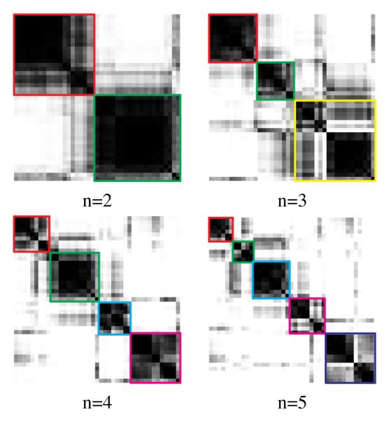
The consensus matrices for different numbers of clusters based on morphological representations are shown. A darker block indicates higher morphological similarity between two cell lines.
Fig. 3.
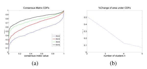
Confidence in the number of clusters: (a) CDF for each cluster and (b) change in CDF as a function of cluster size indicates that three is the optimum number of subpopulations.
Table 1.
Two subpopulations of the the 41 breast cancer cell lines grown in 2D cell culture assay are revealed through consensus clustering. The cell lines listed on the left are mostly luminal, while the cell lines on the right are mostly basal. Luminal and BasalA/B are subpopulations in previous transcript-based clustering results [1].
| Cluster 1 | Cluster 2 | ||
|---|---|---|---|
| Cell line | Type | Cell line | Type |
| SUM185PE | Luminal | AU565 | Luminal |
| ZR751 | Luminal | HCC1143 | BasalA |
| MDAMB415 | Luminal | MCF12A | BasalB |
| BT474 | Luminal | SUM229PE | unknown |
| HCC70 | BasalA | SUM159PT | BasalB |
| MDAMB453 | Luminal | BT549 | BasalB |
| LY2 | Luminal | HCC38 | BasalB |
| MDAMB175VII | Luminal | HBL100 | BasalB |
| MCF7 | Luminal | HCC3153 | BasalA |
| MDAMB361 | Luminal | MDAMB157 | BasalB |
| ZR75B | Luminal | MDAMB231 | BasalB |
| HCC1419 | Unknown | SUM52PE | Luminal |
| HCC1500 | BasalB | HCC1937 | BasalA |
| HCC1806 | Unknown | SUM1315MO2 | BasalB |
| 184A1 | Unknown | HCC1428 | Luminal |
| 184B5 | Unknown | HCC1954 | BasalA |
| MDAMB436 | BasalB | T47D | Luminal |
| MDAMB468 | BasalA | HS578T | BasalB |
| CAMA1 | Luminal | SUM149PT | BasalB |
| UACC812 | Luminal | HCC1395 | Unknown |
| SKBR3 | Luminal | ||
4. CONCLUSION
In this paper, morphometric properties for a panel of breast cell lines were computed, and subpopulations were identified as a result of multidimensional representations of cellular features. The method has been applied to a data set of 41 cell lines grown in 2D cell culture models. We have shown that computed subpopulations correlate with an earlier analysis of transcript data. Our continued research is to couple morphometric data with array-based data (e.g., transcript, methylation), and to compute molecular predictors of each subpopulation.
Acknowledgments
THIS WORK WAS SUPPORTED BY THE DIRECTOR, OFFICE OF SCIENCE, OFFICE OF BIOLOGICAL AND ENVIRONMENTAL RESEARCH, OF THE U.S. DEPARTMENT OF ENERGY UNDER CONTRACT NO. DE-AC02-05CH11231, AND BY THE NATIONAL INSTITUTES OF HEALTH, NATIONAL CANCER INSTITUTE GRANTS P50 CA 58207 AND THE U54 CA 112970.
5. REFERENCES
- [1].Neve R, Chin K, Fridlyand J, Yeh J, Baehner F, Fevr T, Clark L, Bayani N, Coppe J, Tong F. A collection of breast cancer cell lines for the study of functionally distinct cancer subtypes. Cancer Cell. 2006;vol. 10(no 6):515–527. doi: 10.1016/j.ccr.2006.10.008. [DOI] [PMC free article] [PubMed] [Google Scholar]
- [2].Raman S, Maxwell CA, Barcellos-Hoff MH, Parvin B. Geometric approach to segmentation and protein localization in cell culture assays. J Microscopy. 2007;vol. 225(no 1):22–30. doi: 10.1111/j.1365-2818.2007.01712.x. [DOI] [PubMed] [Google Scholar]
- [3].Quan W, Chang H, Parvin B. A delaunay triangulation approach for segmentation clumps of nuclei. Proc IEEE Int Symp on Biomedical Imaging.2009. [Google Scholar]
- [4].Yang Q, Parvin B. Harmonic cut and regularized centroid transform for localization of subcelular structures. IEEE Transaction on Biomedical Engineering. 2003;vol. 50(no 4):469–476. doi: 10.1109/TBME.2003.809493. [DOI] [PubMed] [Google Scholar]
- [5].Han J, Chang H, Andarawewa K, Yaswen P, Barcellos-Hoff MH, Parvin B. Multidimensional profiling of cell surface proteins and nuclear markers. IEEE/ACM Transactions on Computational Biology and Bioinformatics. doi: 10.1109/TCBB.2008.134. in press. [DOI] [PubMed] [Google Scholar]
- [6].Monti S, Tamayo P, Mesirov J, Golub T. Consensus clustering: A resampling-based method for class discovery and visualization of gene expression microarray data. Machine Learning. 2003;vol. 52(no 12):91–118. [Google Scholar]