Competition between collective and individual dynamics

Abstract

Linking microscopic and macroscopic behavior is at the heart of many natural and social sciences. This apparent similarity conceals essential differences across disciplines: Although physical particles are assumed to optimize the global energy, economic agents maximize their own utility. Here, we solve exactly a Schelling-like segregation model, which interpolates continuously between cooperative and individual dynamics. We show that increasing the degree of cooperativity induces a qualitative transition from a segregated phase of low utility toward a mixed phase of high utility. By introducing a simple function that links the individual and global levels, we pave the way to a rigorous approach of a wide class of systems, where dynamics are governed by individual strategies.

The intricate relations between the individual and collective levels are at the heart of many natural and social sciences. Different disciplines wonder how atoms combine to form solids (1, 2), neurons give rise to consciousness (3, 4), or individuals shape societies (5, 6). However, scientific fields assume distinct points of view for defining the “normal”, or “equilibrium”, aggregated state. Physics looks at the collective level, selecting the configurations that minimize the global free energy (2). In contrast, economic agents behave in a selfish way, and equilibrium is attained when no agent can increase its own satisfaction (7). Although similar at first sight, the two approaches lead to radically different outcomes.

In this paper, we illustrate the differences between collective and individual dynamics on an exactly solvable model similar to Schelling's segregation model (8). The model considers individual agents that prefer a mixed environment, with dynamics that lead to segregated or mixed patterns at the global level. A “tax” parameter monitors continuously the agents' degree of altruism or cooperativity, i.e., their consideration of the global welfare. At high degrees of cooperativity, the system is in a mixed phase of maximal utility. As the altruism parameter is decreased, a phase transition occurs, leading to segregation. In this phase, the agents' utilities remain low, in spite of continuous efforts to maximize their satisfaction. This paradoxical result of Schelling's segregation model (8) has generated an abundant literature. Many papers have simulated how the global state depends on specific individual utility functions, as reviewed by ref. 9. There have been attempts at solving Schelling's model analytically, in order to provide more general results (10, 11). However, these approaches are limited to specific utility functions. More recently, physicists have tried to use a statistical physics approach to understand the segregation transition (12 –14). The idea seems promising because statistical physics has successfully bridged the micro–macro gap for physical systems governed by collective dynamics. However, progress was slowed by lack of an appropriate framework allowing for individual dynamics (12). In this paper, we introduce a rigorous generalization of the physicist's free energy, which includes individual dynamics. By introducing a “link” state function that is maximized in the stationary state, we pave the way to analytical treatments of a much wider class of systems where dynamics are governed by individual strategies. Applied to the above Schelling-like segregation model, this approach offers a quantitative solution for very general utility functions.

Model

Our model represents in a schematic way the dynamics of residential moves in a city. For simplicity, we include one type of agent, but our results can readily be generalized to deal with agents of two “colors,” as in the original Schelling model (8) (see Discussion and SI Appendix). The city is divided into Q blocks (Q ≫ 1), each block containing H cells or flats (Fig. 1). We assume that each cell can contain at most one agent, so that the number n _q of agents in a given block q (q = 1,…,Q) satisfies n _q ≤ H, and we introduce the density of agents ρ_q = n _q/H. Each agent has the same utility function u(ρ_q), which describes the degree of satisfaction concerning the density of the block in which he is living. The collective utility is defined as the total utility of all the agents in the city: U(x) = H∑_qρ_q u(ρ_q), where x ≡ {ρ_q} corresponds to the coarse-grained configuration of the city, i.e., the knowledge of the density of each block. For a given x, there is a large number of ways to arrange the agents in the different cells. This number of arrangements is quantified by its logarithm S(x), called the entropy of the configuration x.

Fig. 1.

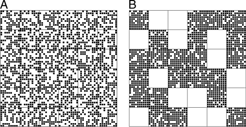
Configurations of a city composed of Q = 36 blocks containing each H = 100 cells, with ρ₀ = 1/2. (A) Mixed state. Stationary state of the city for m = 0.5, α = 1, and T → 0. Agents are distributed homogeneously between the blocks, each of them having a density of 0.5. (B) Segregated configuration. Stationary state of the city for m = 0.5, α = 0, and T → 0. Agents are gathered on 22 blocks of mean density 0.82, the other blocks being empty. In the original Schelling model (8), each agent has a distinct neighborhood, defined by its eight nearest neighbors. Here, we only keep the essential ingredient of blocks of distinct densities. Our model shows the same qualitative behavior as Schelling's but can be solved exactly, thanks to the partial reduction of the agents' heterogeneity.

The dynamical rule allowing the agents to move from one block to another is the following. At each time step, one picks up at random an agent and a vacant cell. Then the agent moves in that empty cell with probability

where x and y are respectively the configurations before and after the move, and G is the gain associated to the proposed move. The positive parameter T is a “temperature” that introduces in a standard way (15) some noise on the decision process. It can be interpreted as the effect of features that are not explicitly included in the utility function but still affect the moving decision (urban facilities, friends, etc.). We write the gain G as

where Δu is the variation of the agent's own utility upon moving and ΔU is the variation of the total utility of all agents. The parameter 0 ≤ α ≤ 1 weights the contribution of the other agents' utility variation in the calculation of the gain G, and it can thus be interpreted as a degree of cooperativity (or altruism). For α = 0, the probability to move only depends on the selfish interest of the chosen agent, which corresponds to the spirit of economic models such as Schelling's. When α = 1, the decision to move only depends on the collective utility change, as in physics models. An economical interpretation could be that individual moves are controlled by a central government, via a tax that internalizes all the externalities (more on this in Discussion). Varying α in a continuous way, one can interpolate between the two limiting behaviors of individual and collective dynamics.

Results

We wish to find the stationary probability distribution Π(x) of the microscopic configurations x. If the gain G can be written as G = ΔV ≡ V(y) − V(x), where V(x) is a function of the configuration x, then the dynamics satisfy the detailed balance (16), and the distribution Π(x) is given by

with F(x) = V(x) + TS(x) and Z a normalization constant. The entropy has for large H the standard expression S(x) = H∑_q s(ρ_q), with

We now need to find the function V(x), if it exists. Given the form in Eq. 2 of G, finding such a function V(x) amounts to finding a “link” function L(x), connecting the individual and collective levels, such that Δu = ΔL. The function V would thus be given by V(x) = (1 − α)L(x) + αU(x). By analogy to the entropy, we assume that L(x) can be written as a sum over the blocks, namely L(x) = H∑_qℓ(ρ_q). Considering a move from a block at density ρ₁ to a block at density ρ₂, ΔL reduces in the large H limit to ℓ′(ρ₂) − ℓ′(ρ₁), where ℓ′ is the derivative of ℓ. The condition Δu = ΔL then leads to the identification ℓ′(ρ) = u(ρ), from which the expression of ℓ(ρ) follows:

As a result, the function F(x) can be expressed in the large H limit as F(x) = H∑_q f(ρ_q), with a block potential f(ρ) given by

The probability Π(x) is dominated by the configurations x = {ρ_q} that maximize the sum ∑_q f(ρ_q) under the constraint of a fixed ρ₀ = Q ⁻¹∑_{q = 1} ^Q ρ_q. To perform this maximization procedure, we follow standard physics methods used in the study of phase transitions [like liquid–vapor coexistence (18)], which can be summarized as follows. If f(ρ) coincides with its concave hull at a given density ρ₀, then the state of the city is homogeneous, and all blocks have a density ρ₀. Otherwise, a phase separation occurs: Some blocks have a density ρ₁ * < ρ₀, whereas the others have a density ρ₂ * > ρ₀ (see SI Appendix).

Interestingly, the potential F = (1 − α)L + αU + TS appears as a generalization of the notion of free energy introduced in physical systems. Mapping the global utility U onto the opposite of the energy of a physical system, it turns out that for α = 1, the maximization of the function U + TS is equivalent to the minimization of the free energy E − TS. For α < 1, the potential F takes into account individual moves through the link function L. Furthermore, the potential F can be calculated for arbitrary utility functions, allowing one to predict analytically the global town state. Such an achievement has thus far eluded individualistic, Schelling-type models, which had to be studied through numerical simulations (9).

To explicitly obtain the equilibrium configurations, one needs to know the specific form of the utility function. To illustrate the dramatic influence of the cooperativity parameter α, we use the asymmetrically peaked utility function (18), which indicates that agents prefer mixed blocks (Fig. 2). The overall town density is fixed at ρ₀ = 1/2 to avoid the trivial utility frustration resulting from the impossibility to attain the optimal equilibrium (ρ_q = 1/2 for all blocks). We also consider for simplicity the limit T → 0 in order to avoid entropy effects. The qualitative behavior of the system is unchanged for ρ₀ ≠ 1/2 or for low values of the temperature, as shown in the SI Appendix.

Fig. 2.

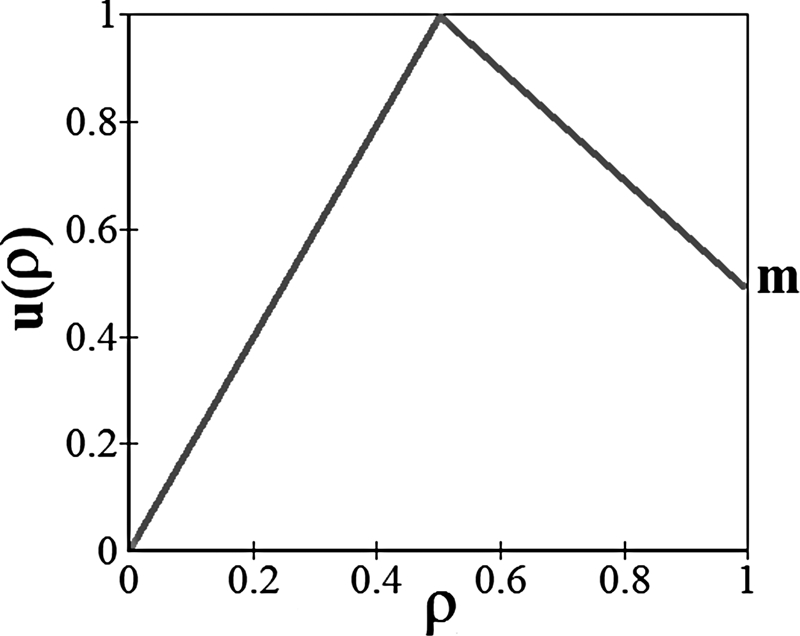
Asymmetrically peaked individual utility as a function of block density. The utility is defined as u(ρ) = 2ρ if ρ ≤ 1/2 and u(ρ) = m + 2(1 − m)(1− ρ) if ρ > 1/2, where 0 < m < 1 is the asymmetry parameter. Agents strictly prefer half-filled neighborhoods (ρ = 1/2). The agents also prefer overcrowded (ρ = 1) neighborhoods to empty ones (ρ = 0).

In the collective case (α = 1), the optimal state corresponds to the configuration that maximizes the global utility, which can be immediately guessed from Fig. 2, namely ρ_q = 1/2 for all q (Fig. 1 A). On the contrary, in the selfish case (α = 0, Fig. 1 B), maximization of the potential F(x) shows that the town settles in a segregated configuration where a fraction of the blocks are empty and the others have a density ρ_s > 1/2. Surprisingly, the city settles in this state of low utility in spite of agents' continuous efforts to maximize their own satisfaction. To understand this frustrated configuration, note that the collective equilibrium (ρ_q = 1/2 for all q) is now an unstable Nash equilibrium at T > 0. The instability can be understood by noting that at T > 0 there is a positive probability that an agent accepts a slight decrease of its utility and leaves a block with density ρ_q = 1/2. The agents remaining in its former block now have a lower utility and are more likely to leave to go to another ρ_q = 1/2 block. This departure creates an avalanche that empties the block as each move away further decreases the utility of the remaining agents. This avalanche stops when the stable (Nash) equilibrium, given by the maximum of the potential, is reached. This state corresponds to a spatially inhomogeneous repartition of agents in the city. To understand the transition between mixed and segregated configurations, it is instructive to calculate the values of both the overall utility and the potential for different values of m (at α = 0). For homogeneous towns, for all m, the normalized collective utility is given by U* = U/(ρ₀ HQ) = u(ρ₀ = 1/2) = 1 and the normalized link function equals L* = L/(ρ₀ HQ) = ℓ(ρ₀)/ρ₀ = 1/2, where ℓ is given in Eq. 5. The values of L* and U* displayed in Table 1 show that the utility of the segregated equilibrium is lower but that its potential is higher, explaining its stability. Note that the gap between the link function values of the homogeneous and segregated configurations increases with m.

Table 1.

Characteristics of the segregated equilibrium

Quantity	m < 2/3	2/3 ≤ m ≤ 1
ρs	$\frac{1}{2}\sqrt{(2-m)∕(1-m)}$	1
U*	$\frac{1}{1+\sqrt{(1-m)∕(2-m)}}$	m
L*	$\frac{1}{1+\sqrt{(1-m)∕(2-m)}}$	1/2 + m/4

The table displays the density ρ_s in the nonempty blocks, the normalized collective utility U* and the normalized link L* of the stationary configurations obtained for α = 0. It is straightforward to check that U*(m) ≤ 1 and L*(m) ≥ 1/2 for m ≤ 1.

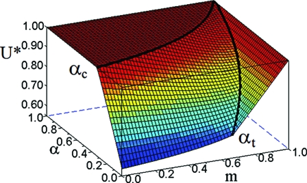
This increase helps one understand why the greater the m, the greater the value of tax parameter necessary to reach the homogeneous configuration. Indeed, the segregated states are separated from mixed states by a phase transition at the critical value α_c = 1/(3 − 2m), which increases with m (Fig. 3). This transition differs from standard equilibrium phase transitions known in physics, which are most often driven by the competition between energy and entropy. Here, the transition is driven by a competition between the collective and individual components of the agents' dynamics. The unsatisfactory global state of the city can be interpreted, from the economic point of view, as an effect of externalities: By moving to increase its utility, an agent may decrease other agents' utilities without taking this into account. From a standard interpretation in terms of Pigouvian tax (19), one expects that α = 1 is necessary to reach the optimal state because by definition this value internalizes all the externalities the agent causes to the others when moving. Our results show that the optimal state is maintained until much lower tax values are reached (for example, α_c = 1/3 at m = 0), a surprising result which deserves further analysis. Another interesting effect is observed for m > 2/3 (Fig. 3). Introducing a small tax has no effect on the overall satisfaction, the utility remaining constant until a threshold level is attained at α_t = (3m − 2)/(6 − 5m).

Fig. 3.

Phase diagram of the global utility as a function of the cooperativity α and the asymmetry m, at T → 0 and ρ₀ = 1/2. The average utility per agent U* = U/(ρ₀ HQ) is calculated by maximizing the potential F(x) for the peaked utility shown in Fig. 2 (see SI Appendix). The plateau at high values of α corresponds to the mixed phase of optimal utility, which is separated from the segregated state by a phase transition arising at α_c = 1/(3 − 2m). The overall picture is qualitatively unchanged for low but finite values of the temperature, (see SI Appendix).

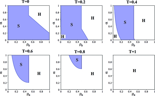
We focused up to now on the zero temperature limit. For low temperatures, the main qualitative conclusions are not modified, as the phase diagram is modified only for extremal values of ρ₀ by entropic contributions. At higher temperatures, the city tends to become homogeneous as the effect of “noise” (i.e., of the features that are not described in the model) dominates over the utility associated with the densities of the blocks (see Fig. 4).

Fig. 4.

Phase diagrams for the asymmetrically peaked individual utility (Fig. 2, with m = 0.8) for different values of T. Increasing the temperature T tends to favor homogeneous states. For small but finite temperatures (roughly T < 0.2), the phase diagram is modified only for extremal values of ρ₀, as expected from the entropic term Ts(ρ) = −Tρln ρ − T(1 − ρ)ln(1 − ρ). As T is increased, the whole diagram is affected by the entropic term. Compared with the T = 0 case, the main change is the appearance of a second homogeneous phase for ρ₀ < 1/2. Although for ρ₀ > 1/2 homogeneity corresponds to the optimal choice for the agents, for ρ₀ < 1/2, collective utility is not maximized in a homogeneous city. The city is homogeneous by noise, not by choice. Note that an increase in α tends to reduce this domain, whereas it tends to increase the homogeneous domain for ρ₀ > 1/2.

Discussion

In the limit α = 0, our model becomes similar to Schelling's segregation model (8), with two main differences: the existence of two types of agents of two colors and the definition of the agent's neighborhoods. We now show that these additional features do not introduce any essential effect.

Let us start by introducing two types of agents with different “colors” (such as red and green). Simple calculations (see SI Appendix) show that for two species that only care about the density of neighbors of their own color, the block potential Eq. 6 becomes

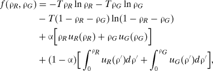with straightforward notations (for example, u _R(ρ_R) represents the utility of a red agent in a block with a density ρ_R of red agents). In the more general case of utility functions depending on both the density of similar and dissimilar neighbors, it is also possible to derive a block potential if the utility functions verify a symmetry constraint. This constraint is not very restrictive, in the sense that no qualitative feature of the model is lost when one restrains the study to utilities that verify it (see SI Appendix).

Finding the equilibrium configurations amounts to finding the set {ρ_qR, ρ_qG}, which maximizes the potential F(x) = ∑_q f(ρ_qR, ρ_qG) with the constraints ∑_qρ_qR = Qρ_0R and ∑_qρ_qG = Qρ_0G, where ρ_0G and ρ_0R represent, respectively, the overall concentration of green and red agents.

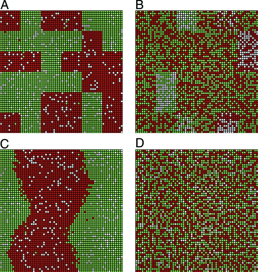
Because of the spatial constraints (the densities of red and green agents in each block q must verify ρ_qR + ρ_qG ≤ 1), the “two populations” model cannot formally be reduced to two independent “one population” models. However, the stationary states can still be easily computed. Let us focus once again on the T → 0 limit and suppose, for example, that ρ_0R = ρ_0G = ρ₀/2. The stationary state depends once again on the values of ρ₀, m, and α. For low values of α, it can be shown that the system settles in segregated states where each block contains only one kind of agent with a density ρ₀ (see Fig. 5 A). For α ≥ α_c, the system settles in mixed states where the density of a group in a block is either 0 or 1/2 (see Fig. 5 B). The reader is referred to SI Appendix for more details.

Fig. 5.

Stationary configurations obtained by simulating the evolution of a city inhabited by an equal number of red and green agents whose preferences are given by the asymmetrically peaked utility function (m = 0.5). The rate of vacant cells (in white) is fixed to 10%. (A and B) The city is divided into blocks of size H = 100. In accordance with the analytic model, a segregated configuration is obtained when α = 0 (A) and a more homogeneous configuration is obtained for α = 1 (B). (C and D) The utility of an agent depends on the local density of similar neighbors computed on the H = 108 nearest cells. Although of different topological nature, a segregated configuration is still obtained for α = 0 (C) and a homogeneous configuration is still obtained for α = 1 (D). In all those simulations, we take T = 0.1. The small amount of noise hence generated, although not changing the nature of the stationary states compared with the case T → 0, conveniently reduces the time of convergence of the system.

We now turn to the difference in agents' neighborhoods. In Schelling's original model, agents' neighbors are defined as their eight nearest neighbors. Our model considers instead predefined blocks of common neighbors. First, it should be noted that there is no decisive argument in favor of either neighborhood definition in terms of the realism of the description of real social neighborhoods. Second, we note that introducing blocks allows for an analytical solution for arbitrary utility functions. This contrasts with the nearest neighbor case, where the best analytical approach solves only a modified model that abandons the individual point of view and is limited to a specific utility function (11). Finally, the simulations presented in Fig. 5 show that the transition from segregated to mixed states is not affected by the choice of the neighborhood's definition. We conclude that the block description is more adapted to this kind of simple modeling, which aims at showing stylized facts as segregation transitions.

Our simple model raises a number of interesting questions about collective or individual points of view. In the purely collective case (α = 1), the stationary state corresponds to the maximization of the average utility, in analogy to the minimization of energy in physics. In the opposite case (α = 0), the stationary state strongly differs from the simple collection of individual optima (20): The optimization strategy based on purely individual dynamics fails, illustrating the unexpected links between micromotives and macrobehavior (21). However, the emergent collective state can be efficiently captured by the maximization of the link function ℓ(ρ) given in Eq. 5, up to constraints in the overall town density. This function intimately connects the individual and global points of view. First, it depends only on the global town configuration (given by the ρ_q), allowing a relatively simple calculation of the equilibrium. At the same time, it can be interpreted as the sum of the individual marginal utilities gained by agents as they progressively fill the city after leaving a reservoir of zero utility. In the stationary state, a maximal value of the potential L is reached. Therefore, no agent can increase its utility by moving (because Δu = ΔL), consistent with the economists' definition of a Nash equilibrium.

Equilibrium statistical mechanics has developed powerful tools to link the microscopic and macroscopic levels. These tools are limited to physical systems, where dynamics are governed by a global quantity such as the total energy. By introducing a link function, analogous to state functions in thermodynamics or potential functions in game theory (22), we have extended the framework of statistical mechanics to a Schelling-like model. Such an approach paves the way to analytical treatments of a much wider class of systems, where dynamics are governed by individual strategies.

References

- 1.Cotterill R. The Cambridge Guide to the Material World. New Rochelle, NY: Cambridge Univ Press; 2008. [Google Scholar]
- 2.Goodstein D. States of Matter. New York: Dover; 1985. [Google Scholar]
- 3.Damasio AR. The Feeling of What Happens. New York: Harcourt Brace; 1995. [Google Scholar]
- 4.Changeux JP. The Physiology of Truth: Neuroscience and Human Knowledge. Cambridge, MA: Belknap Press; 2009. [Google Scholar]
- 5.Smith A. In: An Inquiry into the Nature and Causes of the Wealth of Nations. Strahan W, Cadell T, editors. London: Methuen; 1776. [Google Scholar]
- 6.Latour B. Reassembling the Social: An Introduction to Actor-Network-Theory. New York: Oxford Univ Press; 2007. [Google Scholar]
- 7.Mas–Colell A, Whinston MD, Green JR. Microeconomic Theory. New York: Oxford Univ Press; 1995. [Google Scholar]
- 8.Schelling TC. Dynamic models of segregation. J Math Sociol. 1971;1:143–186. [Google Scholar]
- 9.Clark W, Fossett M. Understanding the social context of the Schelling segregation model. Proc Natl Acad Sci USA. 2008;105:4109–4114. doi: 10.1073/pnas.0708155105. [DOI] [PMC free article] [PubMed] [Google Scholar]
- 10.Pollicott M, Weiss H. The dynamics of Schelling-type segregation models and a nonlinear graph Laplacian variational problem. Adv Appl Math. 2001;27:17–40. [Google Scholar]
- 11.Zhang J. Residential segregation in an all-integrationist world. J Econ Behav Org. 2004;54:533–550. [Google Scholar]
- 12.Dall–Asta L, Castellano C, Marsili M. Statistical physics of the Schelling model of segregation. J Stat Mech Theor Exp. 2008:L07002. [Google Scholar]
- 13.Vinkovic D, Kirman A. A physical analogue of the Schelling model. Proc Natl Acad Sci USA. 2006;103:19261–19265. doi: 10.1073/pnas.0609371103. [DOI] [PMC free article] [PubMed] [Google Scholar]
- 14.Gauvin L, Vannimenus J, Nadal J-P. Phase diagram of a Schelling segregation model. Eur Phys J B. 2009;70:293–304. [Google Scholar]
- 15.Anderson SP, De Palma A, Thisse JF. Discrete Choice Theory of Product Differentiation. Cambridge, MA: MIT Press; 1992. [Google Scholar]
- 16.Evans M, Hanney T. Nonequilibrium statistical mechanics of the zero-range process and related models. J Phys Math Gen. 2005;38:R195–R240. [Google Scholar]
- 17.Callen H. Thermodynamics and an Introduction to Thermostatistics. New York: Wiley; 1985. [Google Scholar]
- 18.Pancs R, Vriend N. Schelling's spatial proximity model of segregation revisited. J Publ Econ. 2007;91:1–24. [Google Scholar]
- 19.Auerbach A. The theory of excess burden and optimal taxation. Handbook Publ Econ. 1985;1:61–127. [Google Scholar]
- 20.Kirman AP. Whom or what does the representative individual represent? J Econ Perspect. 1992;6:117–136. [Google Scholar]
- 21.Schelling TC. Micromotives and Macrobehavior. New York: Norton; 1978. [Google Scholar]
- 22.Monderer D, Shapley L. Potential games. Game Econ Behav. 1996;14:124–143. [Google Scholar]