

Abstract
The genome-wide recombination rate (RR) of a species is often described by one parameter, the ratio between total genetic map length (G) and physical map length (P), measured in centimorgans per megabase (cM/Mb). The value of this parameter varies greatly between species, but the cause for these differences is not entirely clear. A constraining factor of overall RR in a species, which may cause increased RR for smaller chromosomes, is the requirement of at least one chiasma per chromosome (or chromosome arm) per meiosis. In the present study, we quantify the relative excess of recombination events on smaller chromosomes by a linear regression model, which relates the genetic length of chromosomes to their physical length. We find for several species that the two-parameter regression, G = G0 + k · P , provides a better characterization of the relationship between genetic and physical map length than the one-parameter regression that runs through the origin. A nonzero intercept (G0) indicates a relative excess of recombination on smaller chromosomes in a genome. Given G0, the parameter k predicts the increase of genetic map length over the increase of physical map length. The observed values of G0 have a similar magnitude for diverse species, whereas k varies by two orders of magnitude. The implications of this strategy for the genetic maps of human, mouse, rat, chicken, honeybee, worm, and yeast are discussed.
The meiotic recombination rate (RR), defined as the ratio between genetic and physical map length and measured in centimorgans per megabase (cM/Mb), is known to vary widely between the genomes of different species. As a rule of thumb for the human genome, 1 cM genetic map length equals 1 Mb physical map length (see, e.g., Collins and Morton 1998; Ulgen and Li 2005). This rate is about twice as large as the genome-wide RR observed in the mouse genome (Jensen-Seaman et al. 2004), but far less than the RR of 340 cM/Mb that is observed in the yeast genome (Mortimer et al. 1992; Baudat and Nicolas 1997). Understanding of these differences in RR between different species is of fundamental importance for evolutionary and medical genetics (Nachman 2002). In addition to these differences between species, it was also noted that RR differs between chromosomes within a species, with smaller chromosomes showing higher RR (Nachman and Churchill 1996; Broman et al. 1998; International Human Genome Sequencing Consortium 2001; Venter et al. 2001; Kong et al. 2002; Matise et al. 2007). Therefore, species differences in genome-wide RR may be best studied under a model that also considers the intragenomic differences between chromosomes.
From a population genetic perspective, the main role of recombination is the production of new combinations of alleles by shuffling of parental haplotypes, which increases the efficiency of natural selection in theoretical and empirical model systems (Maynard-Smith 1978; Barton and Charlesworth 1998; Otto and Lenormand 2002; Rice 2002). Many recent empirical studies have addressed the question, at which sites in a genome is recombination most likely to occur (Petes 2001; Hey 2004; McVean et al. 2004; Coop 2005; Myers et al. 2005; Mancera et al. 2008). In this context, it was also found that RR evolves extremely fast on a kilobase scale (Ptak et al. 2005; Winckler et al. 2005) and that historical recombination hotspots are associated with specific gene functions in human, which was hypothesized to indicate an influence of natural selection on hotspot locations (Freudenberg et al. 2007; The International HapMap Consortium 2007). When RR is examined at a megabase scale instead of a kilobase scale, the evolution of local RR is more constrained (Myers et al. 2005) and differs much less between closely related species, such as human and chimpanzees (Ptak et al. 2005; Winckler et al. 2005). However, the mechanism behind this conservation of RR on the larger scale is unclear. One contributing explanation could be the requirement of a minimal or fixed number of chiasmata per chromosome during meiosis to stabilize homologous chromosome pairs (Mather 1938).
The question of how many chiasmata are exactly required per chromosome or per chromosome arm has not been resolved yet and might not have a generally valid answer (Laurie and Hultén 1985; Lynn et al. 2004). Nevertheless, these meiotic constraints can explain the excess of recombination on shorter chromosomes. Consistent with an influence of karyotype on overall recombination rate, a correlation was found between the number of chromosome arms in a genome and the genetic map length (De Villena and Sapienza 2001a). Altered recombination may lead to aneuploidy (Hassold and Hunt 2001; Lynn et al. 2004), which may impose strong selective constraints and explain the tight relationship between karyotype structure and recombination rate (De Villena and Sapienza 2001b; Dumas and Britton-Davidian 2002).
On the other hand, domesticated plants and animals show evidence for increased chiasma formation (Burt and Bell 1987), which suggests that there exist additional determinants of genome-wide RR than karyotype. For instance, the level of interference in chiasma formation could differ between species (Broman et al. 2002). Therefore, it would be useful to apply a formal method that separates the contribution of karyotype structure from the relationship between physical and genetic map length. This is not accomplished by the genome-wide cM/Mb ratio: Although the cM/Mb ratio is a convenient single-parameter measurement, it does not model the higher contribution of smaller chromosomes to the genome-wide RR of a species.
To address this problem and better understand the overall RR of a genome, we propose a novel strategy that explicitly models, if and to what extent, the overall RR in a genome is influenced by the relative excess of recombination on smaller chromosomes. This proposed two-parameter strategy takes into account that a certain minimal amount of recombination is required to maintain genome integrity during meiosis (Mather 1938) and that a genome therefore has minimal genetic map length. This idea becomes more clear if we use a statistical regression framework to compare the proposed strategy with the one-parameter strategy that is typically applied to shorter scales than the chromosome scale. Since the one-parameter characterization of RR implies that genetic length is proportional to the physical length and recombination events occur independently on different chromosomes, the cM/Mb ratio is the slope of the linear regression of genetic lengths of chromosomes over their sequence lengths, with the requirement that the regression line goes through the origin. In our new approach, we drop the requirement that the regression line must go through the origin by using two parameters to fit the genome-wide genetic map information at the chromosomal scale.
From a biological perspective, the one-parameter model considers the length of the genetic map of a genome to be determined by the length of the underlying physical map and the species-specific RR. Building on this, the two-parameter model also includes a separate effect of karyotype structure that may produce a disproportional distribution of recombination events over chromosomes of different length. Under the two-parameter model, the value of the y-intercept quantifies the relative excess of recombination events on a hypothetical chromosome with length zero, whereas the slope of the regression measures the increase of genetic with physical map length in the same way as the one-parameter model. Our results show that in human, as well as other species, the two-parameter regression provides a much better fit for describing the genetic map length of chromosomes.
Results
A two-parameter regression model fits the genetic map length of human chromosomes better than the one-parameter model
To look for systematic differences in the recombination rate between human chromosomes, we started by reproducing the Marey map (Chakravarti 1991; Rezvoy et al. 2007), a cumulative plot similar to those used in DNA sequence representation or analysis (Li 1997; Grigoriev 1998), for 22 human autosomes and 34 arms of metacentric chromosomes (Supplemental Fig. S1). The chromosome-scale or chromosome-arm-scale recombination rate may be defined as the slope of a straight line that links the first and the last marker. For smaller chromosomes or chromosome arms, the endpoints in the Marey map tend to lie above the line with a slope equal to 1 (cM = Mb), that is, smaller chromosomes (−arms) have larger cM/Mb ratios (see also Fig. 16 of International Human Genome Sequencing Consortium 2001 and Table 12 of Venter et al. 2001).
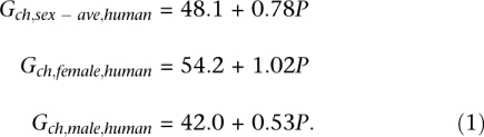
We next regressed the genetic map length of chromosomes over their physical map length (Fig. 1A; a similar plot can be found in Housworth and Stahl 2003). When sex-averaged, female and male genetic lengths are fitted separately, the three regression lines are described by:
 |
The normality assumption of regression residuals was tested graphically by a QQ plot (Supplemental Fig. S2), and the normality condition does not seem to be violated.
Figure 1.

Two-parameter regression of human genetic length over physical length. (A) Analysis at the chromosome scale. (Squares) Female, (open circles) male, and (solid circles) sex-averaged genetic length of each chromosome (in centimorgans, cM) is plotted against its physical length (in megabases, Mb). The least-square regression lines are: y = 54.2 + 1.02x (female), y = 42.0 + 0.52x (male), and y = 48.1 + 0.78x (sex average). (B) Analysis of metacentric chromosome at the chromosome-arm scale. The best-fit regression lines are: y = 29.0 + 1.05x (female), y = 27.1 + 0.48x (male), and y = 28.0 + 0.77x (sex average).
Equation 1 shows that the y-intercept G0 for female data is 29% larger than for male data, whereas the slope k is 92% larger. Thus, the different lengths of the male and female maps mainly manifest as a different slope and less so as a different y-intercept. As can be seen from Figure 1A, all human chromosomes exceed the minimal length of 50 cM both for the male and the female genetic maps.
To test the robustness of the y-intercept value, we added random noise to the genetic map length and repeated the regression analysis. The histogram of 50,000 y-intercepts from this procedure is shown in Supplemental Figure S3. Although values of G0 range from 35 to 60, they are all far from zero.
We next repeated the analysis using chromosome arms instead of full chromosomes as separate data points (Fig. 1B). This leads to the regression equations:
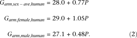 |
The y-intercepts at chromosome-arm-scale regression is now reduced to somewhat more than half of the intercept at the full-chromosome scale. This reduction shows that cytogenetic constraints exert a smaller influence on the chromosome-arm scale than on the full-chromosome scale.
Several methods can be used to show that the two-parameter regression model fits the data better than the one-parameter regressions. To this end, we first compared the coefficient of determination R2, which is the proportion of variability explained by the regression model. The observed R2 values of the one-parameter regression range between 0.48 and 0.87, whereas the R2 values of the two-parameter regressions range between 0.86 and 0.98 (Table 1), indicating that the two-parameter regression explains more of the variability in the data.
Table 1.
Comparison of the two-parameter and one-parameter regression models for human genetic length, at the chromosome scale (22 data points) and the chromosome-arm scale (34 data points)

Comparison coefficient of determination (R2) for two- and one-parameter regressions, and P-value for testing the null hypothesis of zero y-intercept.
We further cast the comparison between the one- and two-parameter regression as a model selection problem. Two such model comparison strategies are provided by the Akaike information criterion (AIC) (Akaike 1974) and Bayesian information criterion (BIC) (Schwarz 1978). Both AIC and BIC values for the two-parameter regression model are smaller than those for the one-parameter model, indicating a better statistical model (Supplemental Table S1).
Finally, we tested the null hypothesis that G0 is zero. The P-values in this test range between 10−13 and 10−8 (Table 1). Because the null hypothesis is that all chromosomes have the same RR, a simulated distribution of G0 can be obtained from the regression over data that are obtained by the permuting of chromosome-specific cM/Mb ratios, while leaving the physical chromosome length unchanged. Out of 50,000 such permutations, only two showed a G0 value that is larger than the observed value of 48.1 (for sex-averaged full chromosome data), corresponding to a P-value of 4 × 10⁻⁵. To summarize, all evaluation methods support the conclusion that the two-parameter regression model is better than the one-parameter model.
As the deCODE data were published more than 6 years ago, we further tested the chromosome-scale regression strategy on a more recent data set, the Rutgers Map v.2 (Matise et al. 2007). The regression lines are G = 53.33 + 0.87P (sex-average), G = 50.29 + 1.19P (female), and G = 57.58 + 0.57P (male), respectively. These results are consistent with the parameter estimations in Equation 1, again showing that male and female data differ more in the slope than in the y-intercept.
Two other quantities can be derived from G0 that help to interpret the y-intercept parameter. The first is the physical length Pmin on the regression line that corresponds to a specified minimum genetic length Gmin such that Gmin = G0 + kPmin. If we set Gmin = 50 cM, then we obtain Pmin = 2.45 Mb for sex-averaged chromosome data. One may assume that for any hypothetical chromosome with P < Pmin, its genetic length G remains constant at 50 cM and does not decrease for shorter chromosome length. As the second quantity of interest, we define the percentage of genetic length that is explained by the inclusion of G0 into the model as:  . For the sex-averaged data, we find that α = 31% of variability is explained by the y-intercept. This value can also be obtained from the decomposition of
  : 1.13 = 0.35 + 0.78, because 0.35/1.13 = 31%. The relatively large percentage value once again highlights the importance of the y-intercept G0 for modeling chromosome-scale recombination rate in human.
Different intercept but similar slope in the two-parameter regression models for rat and mouse chromosomes
Both the rat (Rattus norvegicus) and the mouse (Mus musculus) genomes are known to have lower recombination rates than human (Jensen-Seaman et al. 2004), with rat having a higher overall RR than mouse. The rat genome has a roughly equal physical map length, but contains one more chromosome (n = 20) than the mouse genome (n = 19). Furthermore, rat chromosomes show a greater heterogeneity in their physical length, and one may hypothesize that these karyotype differences contribute to the somewhat higher RR in rat (0.62 cM/Mb vs. 0.57 cM/Mb in mouse). The regression models of the sex-averaged genetic length of rat and mouse chromosomes over their sequence lengths (Fig. 2A) are:
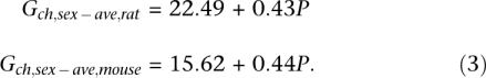 |
These models display a similar slope, and the different overall RR of rat and mouse mainly manifests as a different intercept value G0.
Figure 2.

The genetic length (in centimorgans, cM) vs. physical length (in megabases, Mb) plotted for five genomes. (A) (×) Mouse (Mus musculus) and (○) rat (Rattus norvegicus). [Data source: Table 1 of Jensen-Seaman et al. 2004.] The regression lines are: y = 15.62 + 0.44x (mouse), y = 22.49 + 0.43x (rat). (B) Chicken (Gallus gallus). [Source: old data (year 2004, ○) are from Supplemental Table S2 of the International Chicken Genome Sequencing Consortium (2004); new data (year 2008, ×) are from Table 1 of Groenen et al. (2009).] The regression line is y = 34.68 + 2.79x (old data) and y = 34.23 + 2.04x (new data). (C) Honeybee (Apis mellifera). [Source: Table 2 of Beye et al. 2006.] The regression line is y = −4.22 + 23.49x. (D) Budding yeast (Saccharomyces cerevisiae). [Source: http://downloads.yeastgenome.org/chromosomal_feature/SGD_features.tab.] The regression line is y = 49.12 + 287.74x.
Testing G0 = 0 for the rat genome is significant (P-value = 0.0012), whereas testing G0 = 0 for the mouse genome (the fitted G0 value for mouse is 69% of that for rat) is not significant (P-value = 0.11). AIC/BIC calculation confirms that the two-parameter regression is a convincingly better model for rat than the one-parameter regression, whereas this barely holds for the mouse data (Supplemental Table S1). Thus, the mouse genome displays a nonsignificant excess of recombination on smaller chromosomes, which is consistent with the smaller variation of chromosome size in the mouse genome. The greater y-intercept for the rat genome supports the hypothesis that cytogenetic factors contribute more to the genetic map length of rat than mouse.
Because the rat karyotype consists of both metacentric and acrocentric chromosomes, we repeated the analysis after splitting all metacentric rat chromosome into two parts, based on the location of the centromere. Different from the human genome, for the rat genome this mainly affects the smaller chromosomes, which are often metacentric. The regression line is now described by G = 7.48 + 0.52P, and testing the intercept is still significant (P-value = 0.024), although at a less stringent level. Thus, at the scale of chromosome arms, the likelihood of crossovers is more determined by physical length and less influenced by any obligate recombination requirements.
Recombination rate of small and large chromosomes in the chicken genome
The chicken (Gallus gallus) genome consists of both large (macro-) and small (micro-) chromosomes (Smith et al. 2000; International Chicken Genome Sequencing Consortium 2004), with length ranging from a few megabases to close to 200 Mb. The two-parameter regression model for the chicken genetic data in Figure 2B leads to:
In this regression model, the nonzero intercept is significant with a P-value of 1.33 × 10⁻⁷, and there is a considerable difference of AIC/BIC for the one- and two-parameter regression favoring the two-parameter model (Supplemental Table S1). Both coefficients of determination for the two- and one-parameter regressions attain a high value: 0.98 and 0.93, respectively. A reason that the one-parameter regression only marginally reduces the R2 value is given by the fact that larger chromosomes contribute much more to the total variance, which is equally well captured by the one-parameter model. Thus, two of the three methods confirm a relative excess of recombination on short chromosomes.
However, the orders-of-magnitude difference between the sizes of chicken chromosomes raises the question of the robustness of the regression. From International Chicken Genome Sequencing Consortium (2004) and Supplemental Figure S4, it is clear that the genetic length reaches a plateau at the level of 50 cM for microchromosomes smaller than 8 Mb. When chromosomes below a certain length threshold are discarded from the regression analysis, the y-intercept value changes slightly, but not dramatically. For example, if the length thresholds for removal are 8 Mb and 25 Mb, G0 for Equation 4 decreases to 32.95 and 31.88. When the regression model is only fitted to the five largest chromosomes (longer than 50 Mb), the model parameters are G = 26.22 + 2.84P. On the other hand, if we remove the largest five chromosomes, the regression line is G = 31.86 + 3.01P.
To see how the quality of the map distance measurements may influence these results, we next looked at the recently updated chicken map (Groenen et al. 2009), which contains more genetic markers and higher marker density. Applying the two-parameter regression leads to
As can be seen, the overall reduction of RR as compared to the older map (International Chicken Genome Sequencing Consortium 2004) mainly manifests as a reduced estimate of k, whereas the estimate of G0 remains almost unchanged.
Exceptionally high recombination on the largest honeybee chromosome leads to a better fit of the one-parameter than the two-parameter model
Notably, the two-parameter regression does not provide a better fit for the genetic map data from honeybee (Apis mellifera) (Beye et al. 2006) than the one-parameter model. When plotting the genetic length over physical length (Fig. 2C), the y-intercept of the regression line does not significantly differ from zero (P-value = 0.81):
The coefficient of determination for both the two- and one-parameter regression is ∼0.95. In contrast to other genomes, AIC/BIC analysis favors the one-parameter regression model (Supplemental Table S1).
As can be seen from Figure 2C, the longest chromosome (chromosome 1) is four times the length of the shortest chromosome, and the regression result may depend on the presence of this “outlier.” To check this possibility, we repeated the analysis after chromosome 1 was removed, which led to the regression equation: G = 28.71 + 20.36P. However, also in this model, testing G0 = 0 is not significant (P-value = 0.37), both the two- and one-parameter regressions exhibit similar coefficients of determination (R2 = 0.80, 0.79), and the zero-intercept regression is still the better model according to AIC/BIC analysis (Supplemental Table S1). Therefore, different from other species, the honeybee genome does not display any significant excess of recombination on smaller chromosomes.
Two-parameter regression at much shorter length scales: The example of budding yeast
Yeast (Saccharomyces cerevisiae) has been extensively used to study the molecular machinery of recombination, and it has a much smaller (∼12 Mb) and more compact genome (Cherry et al. 1997). Although the physical length of yeast chromosomes only ranges from 200 kb to 1.5 Mb, their genetic length is between 100 and 500 cM, even longer than the genetic length of human chromosomes. The best-fitting regression line for the yeast genetic map is (Fig. 2D):
The nonzero y-intercept is significant (P-value = 0.009). The two-parameter regression is superior to the one-parameter model as judged by AIC/BIC (Supplemental Table S1). The value of the y-intercept, 49.12 cM, is very close to 50 cM, which corresponds to almost one crossing-over event for a hypothetical chromosome of physical length of zero.
The extremely high recombination rate in the yeast genome is surprising. From the molecular perspective, one can speculate about various hypotheses, such as a different meiotic regulatory system that makes a denser spatial distribution of chiasmata possible; a lack of secondary chromatin structure as compared to higher organisms so that the actual physical distance between two locations on a chromosome is more or less equal to the linear sequence distance; or the lack of another supporting mechanism to hold chromatids together so that more chiasmata per chromosome arm are required for proper chromosome segregation. On the other hand, the y-intercept of the regression has a similar magnitude as that observed for higher organisms, indicating a similar relative excess of recombination on smaller chromosomes.
The difference between the central gene cluster and telomeric regions in worm genome is due to a difference in G0
Finally, we used genetic map data from the worm Caenorhabditis elegans to show that the two-parameter regression strategy can also be useful to compare different regions within a genome. The chromosomes of C. elegans are unusual, because discrete centromeres are missing and the chromosomes are holocentric, that is, microtubules attach at many sites for chromatid segregation (Tyler-Smith and Floridia 2000). Accordingly, the Marey map analysis of the worm genome indicates that each worm chromosome can be partitioned in three regions: the central gene-rich region with a low recombination rate and two distal telomeric regions with high recombination rates (Barnes et al. 1995). Therefore, we separately performed the regression analysis of genetic length over physical length for these two types of regions (Fig. 3). The fitted regression coefficients are:
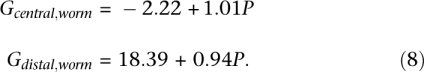 |
Figure 3.

The cM-Mb plot using the physical and genetic length of central gene clusters (five data points) and distal arms (10 data points) of five worm (Caenorhabditis elegans) chromosomes (Table 1 of Barnes et al. 1995). The best-fitting regression lines are y = 18.39 + 0.94x for the (×) distal/telomeric arms and y = −2.22 + 1.01x for the (○) central gene cluster regions.
Within the single-parameter framework without the intercept term G0, the two types of regions would have a very different cM/Mb ratio: 4.57 for telomeric regions, 0.68 for central regions. However, when allowing nonzero G0 values, the two regions display similar slope values, 1.01 and 0.94. This indicates a constant excess of recombination in the distal region as compared to the central region in C. elegans, which is combined with a similar incremental cM/Mb ratio. Thus, after accounting for a fixed amount of recombination in a distal chromosome region, the likelihood of any additional recombination depends on similar strength on physical length in distal and central regions.
As a note of caution, one may point out that the regression coefficient in Equation 8 is obtained from only a few data points. Nevertheless, further regression diagnostics supports our conclusion. For example, testing G0 = 0 is significant for the distal regions (P-value = 0.006), but not significant for central regions (P-value = 0.57). AIC/BIC analyses lead to the same conclusion (Supplemental Table S1).
Discussion
Our results show that instead of the simpler genetic-to-physical length ratio, the relationship between the physical and genetic map length at chromosome scale is better described by a statistical model that contains a second parameter G0, which is the y-intercept of the regression of genetic map length over the physical chromosome length. A conceptually similar approach was used earlier in measuring the genome-wide recombination rate of a species by counting the chiasmata on each chromosome in excess of one (Burt and Bell 1987).
The consideration of this intercept parameter is important, because karyotype structure has been established as an important determinant of genome-wide RR (DeVillena and Sapienza 2001a; Coop 2005) and smaller chromosomes display higher RR (International Human Genome Sequencing Consortium 2001; International Chicken Genome Sequencing Consortium 2004). Our proposed two-parameter model provides a formal expression of this size dependency of RR: RR = G/P = k + G0/P; that is, a constant term k plus a second term that increases for smaller chromosome sizes P (if G0 is positive). This is what we observe for human, mouse, rat, chicken, and yeast genomes. When writing G0 as G0 = G − kP, the y-intercept measures the amount of recombination after the physical map length has been accounted for. Therefore, one would expect that the total map length G of a chromosome increases by G0 after splitting it up into two separate parts. In fact, this has already been quantitatively observed for the experimental alteration of yeast chromosome I (Kaback et al. 1992).
When comparing RR between species, the usage of k instead of the genome-wide cM/Mb ratio will reduce the influence of karyotype differences on the result. This was also the intention behind the counting of chiasmata per chromosome in excess of one (Burt and Bell 1987). In our study, the order of species remains unchanged, whether ranked by k or by cM/Mb ratio. However, owing to the different values of k, we cannot use a single regression line to model the genetic–physical length relationship across species. Thus, a molecular mechanism must exist that drives, within a particular species, the proportional increase of genetic over physical map length. This mechanism might typically act with weaker strength in larger genomes, which could contribute to the inverse correlation between genome size and RR (Lynch 2006).
Among mammals, it was furthermore found that RR is more similar for more closely related species (Dumont and Payseur 2008), which could be partly caused by their similar karyotypes. It might be interesting to test where in the phylogenetic tree the signal might be altered, when using k instead of the genome-wide cM/Mb ratio. In this context, it is also important that genome-wide RR typically differs between genders and individuals (Broman et al.1998; Kong et al. 2002, 2004; Cheung et al. 2007; Petkov et al. 2007). The biological factors that were invoked as possible explanations, such as differences in synaptonemal complex formation or crossover interference, may be more plastic than karyotype structure. The respective strength of these factors could also contribute to species differences and may be better measured by using k than by using the genome-wide cM/Mb ratio.
If k were equal to zero with the obligate chiasma requirement holding true, then G0 would be required to be 50 cM. This pattern can be observed for female opossum (Monodelphis domestica), where each chromosome acquires exactly one crossover near one of its telomeres (see Supplemental Fig. S5; Mikkelsen et al. 2007). Similarly, very small chromosomes may always acquire exactly one crossover, despite reduced chromosome size, as seen for the microchromosomes in the chicken genome. In order to predict the transition from this plateau to the linear regression, we derived the minimum physical length parameter Pmin from a given Gmin and the estimated regression parameters. Note that if both physical and genetic lengths are measured as those in excess of Pmin and Gmin, their ratio is exactly equal to k: (G − Gmin)/(P − Pmin) = (G − Gmin)/(P − (Gmin − G0)/k) = (G − Gmin)/((kP + G0 − Gmin)/k) = k.
Because reduced recombination may result in aneuploidy of smaller chromosomes (Warren et al. 1987; Brown et al. 2000), it is conceivable that the length of smaller chromosomes could influence genome-wide RR by introducing a lower bound for the propensity for chiasma formation in a species. Our analysis supports the size of the smaller chromosomes as a strong determinant of genome-wide RR for the six genomes studied in this paper (Supplemental Fig. S6). In log–log scale, the correlation coefficient between RR and the shortest chromosome length is −0.92 (P-value = 0.008). If the recombination rate is measured by k, in log–log scale the correlation coefficient is −0.91 (P-value = 0.01). This correlation is nearly as strong as the reported correlation between RR and the total physical length for more than 100 genomes (cc = −0.99, P-value = 0.0003 on log–log scale) as reported in Lynch (2006). Obviously, data on more species are needed for a more conclusive analysis. Nevertheless, it may be interesting to point out that the genome with the lowest known recombination rate, opossum, lacks any short chromosome (Mikkelsen et al. 2007; Samollow et al. 2007).
Obviously, any genome-wide analysis relies on the availability of high-quality data. We are convinced that the data used in this study are of sufficient quality to study recombination on the chromosomal scale. However, some error might be introduced by the fact that the used genetic maps are not perfect and, in particular for telomeres, missing some data. This can be seen for the chicken genomes, where the two chromosomes fall below the minimum genetic length of 50 cM in the older map and climb to ∼50 cM in the newer map (Supplemental Fig. S4). Data selectively missing crossovers at the telomeres might lead to an underestimation of G0 in the regression model.
We note that we restricted our analysis to chromosomes or chromosome arms. If the genetic length is regressed over the length of much smaller regions, the coefficient of determination R2 is expected to be much lower owing to a mixture of recombination hotspots and coldspots. From a biological perspective, we also would not expect a positive G0 value in such a regression, because there is no requirement for a megabase-sized region to have at least one chiasma to maintain meiotic integrity.
In summary, we find that the introduction of the G0 parameter helps us to understand the recombination rate differences between species, because it separates the effect of the requirement for at least one chiasma formation on smaller chromosomes from the factors that determine the amount of recombination on larger chromosomes. More specifically, the partitioning of the chromosome-scale recombination rate leads to the following list of conclusions:
Human male–female RR differences disproportionately affect larger chromosomes;
The higher recombination rate in the rat genome as compared to the mouse genome is likely to be caused by the higher number of smaller chromosomes that constitute the rat karyotype;
Both chicken micro- and macrochromosomes display a high RR, and the extraordinarily high RR of some microchromosomes does not lead to an extraordinary excess of recombination on smaller chromosomes;
The honeybee genome does not display any significant excess of recombination on smaller chromosomes;
Yeast displays a relative excess of recombination on smaller chromosomes that is similar to higher organisms, despite its outstandingly high overall recombination rate; and
Recombination of the worm genome mainly occurs in telomeric regions, and given one recombination per chromosome, the likelihood of a second recombination is determined by physical map length.
These examples demonstrate that the proposed statistical framework allows us to pinpoint differences in the genomic recombination rate, which should be useful for the further study of the genome-wide recombination rate as a quantitative trait of fundamental importance.
Methods
Genetic map data
The human genetic map was obtained from Kong et al. (2002) that uses 5136 microsatellite markers with 1257 meiotic events, and is estimated from pedigree data (Supplemental Table E). The rat (R. norvegicus) and mouse (M. musculus) genetic map data were obtained from Table 1 of Jensen-Seaman et al. (2004), based on 2305 markers in rat and 4880 markers in mouse. The two chicken (G. gallus) genetic maps were obtained from Supplemental Table S2 of International Chicken Genome Sequencing Consortium (2004), which is built from 1471 markers, and from Table 1 of Groenen et al. (2009), built from 9258 markers. The honeybee (A. mellifera) genetic map was obtained from Table 2 of Beye et al. (2006) based on 1500 markers. The budding yeast (S. cerevisiae) genetic map was downloaded from http://downloads.yeastgenome.org/chromosomal_feature/SGD_features.tab. The worm (C. elegans) physical and genetic lengths of central “gene clusters” and distal “arms” were obtained from Table 1 of Barnes et al. (1995), based on 168 markers.
Measuring how good a linear regression is by coefficient of determination
Regression analyses were carried out by the lm( ) subroutine in the R statistical package. For genetic lengths, {Gi} (i = 1,2,··· n, e.g., n = 22 for the chromosome-scale regression and n = 34 for the chromosome-arm-scale regression), one can regress them over sequence lengths {Pi} (i = 1,2, ··· n) allowing y-intercept (nonzero G when P approaches 0):
or, without the y-intercept (G approaches 0 as P approaches 0):
How good a linear regression model fits the data can be measured by the coefficient of determination R2, which is the proportion of variability that is explained by the model. More specifically, if  is the total sum of squares of the genetic lengths of chromosomes, the term
  for allowing nonzero y-intercept, or the term
  for not allowing y-intercept, is the residual sum of squares (RSS), then
Model selection by Akaike information criterion
The Akaike information criterion (AIC) (Akaike 1974) of a statistical model is defined as 2p − 2log(L), where p is the number of parameters in the model, and L is the maximum likelihood estimated from the data. Similarly, the Bayesian information criterion (BIC) (Schwarz 1978) is defined as log(n)p − 2log(L), where n is the number of samples used to calculate the likelihood. For linear regression, AIC/BIC is related to the residual sum of squares (RSS) according to Venables and Ripley (1999) by:
 |
where n is the number of sample points for the regression analysis. Between two statistical models that are fitted to the same data set, the model with a smaller AIC/BIC value is considered to be better than the model with a larger AIC/BIC value.
For the comparison between the two- and one-parameter regressions, we have:
 |
If the second term, n log(RSS1/RSS2), is larger than 2 [for AIC, or long(n)for BIC], then the two-parameter regression can be seen as the better model than the single-parameter regression.
Quantities derived from G0
The linear relationship between G and P cannot extend to the physical length of zero, if the y-intercept is greater than zero and the obligate chiasma requirement holds. Therefore, a point Pmin must exist below which genetic map length remains constant at Gmin, independent from the actual physical map length of a chromosome. We can define this transition point as follows: Pmin is the physical length for which the regression line crosses the horizontal line defined by the minimum genetic length Gmin, thus Pmin = (Gmin − G0)/k.
Another derived quantity is the genome-wide percentage of genetic length that is explained by G0. For a single chromosome (i), this percentage is αi ≡ G0/(G0 + kPi). For the whole genome, it is  , where n is the number of chromosomes. This definition of α is valid only when the y-intercept is positive (G0 > 0).
Acknowledgments
We thank Alejandro Morales for participating in the initial stage of this work; Tara Matise, Zhiliang Hu, Hong Ma, and Oliver Clay for discussions; and the anonymous reviewers for their valuable comments and suggestions. J.F. was supported by an NARSAD Young Investigator award.
Footnotes
[Supplemental material is available online at http://www.genome.org.]
Article published online before print. Article and publication date are at http://www.genome.org/cgi/doi/10.1101/gr.092676.109.
References
- Akaike H. A new look at statistical model identification. IEEE Trans Automat Contr. 1974;19:716–722. [Google Scholar]
- Barnes TM, Kohara Y, Coulson A, Hekimi S. Meiotic recombination, noncoding DNA and genomic organization in Caenorhabditis elegans. Genetics. 1995;141:159–179. doi: 10.1093/genetics/141.1.159. [DOI] [PMC free article] [PubMed] [Google Scholar]
- Barton NH, Charlesworth B. Why sex and recombination? Science. 1998;281:1986–1990. [PubMed] [Google Scholar]
- Baudat F, Nicolas A. Clustering of meiotic double-strand breaks on yeast chromosome III. Proc Natl Acad Sci. 1997;94:5213–5218. doi: 10.1073/pnas.94.10.5213. [DOI] [PMC free article] [PubMed] [Google Scholar]
- Beye M, Gattermeier I, Hasselmann M, Gempe T, Schioett M, Baines JF, Schlipalius D, Mougel F, Emore C, Rueppell O, et al. Exceptionally high levels of recombination across the honey bee genome. Genome Res. 2006;16:1339–1344. doi: 10.1101/gr.5680406. [DOI] [PMC free article] [PubMed] [Google Scholar]
- Broman KW, Murray JC, Sheffield VC, White RL, Weber JL. Comprehensive human genetic maps: Individual and sex-specific variation in recombination. Am J Hum Genet. 1998;63:861–869. doi: 10.1086/302011. [DOI] [PMC free article] [PubMed] [Google Scholar]
- Broman KW, Rowe LB, Churchill GA, Paigen K. Crossover interference in the mouse. Genetics. 2002;160:1123–1131. doi: 10.1093/genetics/160.3.1123. [DOI] [PMC free article] [PubMed] [Google Scholar]
- Brown AS, Feingold E, Broman KW, Sherman SL. Genome-wide variation in recombination in female meiosis: A risk factor for non-disjunction of chromosome 21. Hum Mol Genet. 2000;9:515–523. doi: 10.1093/hmg/9.4.515. [DOI] [PubMed] [Google Scholar]
- Burt A, Bell G. Mammalian chiasma frequencies as a test of two theories of recombinations. Nature. 1987;326:803–805. doi: 10.1038/326803a0. [DOI] [PubMed] [Google Scholar]
- Chakravarti A. A graphical representation of genetic and physical maps: The Marey map. Genomics. 1991;11:219–222. doi: 10.1016/0888-7543(91)90123-v. [DOI] [PubMed] [Google Scholar]
- Cherry JM, Ball C, Weng S, Juvik G, Schmit R, Adler C, Dunn B, Dwight S, Riles L, Mortimer RK. Genetic and physical maps of Saccharomyces cerevisiae. Nature. 1997;387:67–74. [PMC free article] [PubMed] [Google Scholar]
- Cheung VG, Burdick JT, Hirschmann D, Morley M. Polymorphic variation in human meiotic recombination. Am J Hum Genet. 2007;80:526–530. doi: 10.1086/512131. [DOI] [PMC free article] [PubMed] [Google Scholar]
- Collins A, Morton NE. Mapping a disease locus by allelic-association. Proc Natl Acad Sci. 1998;95:1741–1745. doi: 10.1073/pnas.95.4.1741. [DOI] [PMC free article] [PubMed] [Google Scholar]
- Coop G. Can a genome change its (hot)spots? Trends Ecol Evol. 2005;20:643–645. doi: 10.1016/j.tree.2005.10.006. [DOI] [PMC free article] [PubMed] [Google Scholar]
- De Villena FPM, Sapienza C. Recombination is proportional to the number of chromosome arms in mammals. Mamm Genome. 2001a;12:318–322. doi: 10.1007/s003350020005. [DOI] [PubMed] [Google Scholar]
- De Villena FPM, Sapienza C. Female meiosis drives karyotypic evolution in mammals. Genetics. 2001b;159:1179–1189. doi: 10.1093/genetics/159.3.1179. [DOI] [PMC free article] [PubMed] [Google Scholar]
- Dumas D, Britton-Davidian J. Chromosomal rearrangements and evolution of recombination: Comparison of chiasma distribution patterns in standard and robertsonian populations of the house mouse. Genetics. 2002;162:1355–1366. doi: 10.1093/genetics/162.3.1355. [DOI] [PMC free article] [PubMed] [Google Scholar]
- Dumont BL, Payseur BA. Evolution of the genomic rate of recombination in mammals. Evolution. 2008;62:276–294. doi: 10.1111/j.1558-5646.2007.00278.x. [DOI] [PubMed] [Google Scholar]
- Freudenberg J, Fu YH, Ptácek LJ. Enrichment of HapMap recombination hotspot predictions around human nervous system genes: Evidence for positive selection? Eur J Hum Genet. 2007;15:1071–1078. doi: 10.1038/sj.ejhg.5201876. [DOI] [PubMed] [Google Scholar]
- Grigoriev A. Analyzing genomes with cumulative skew diagrams. Nucleic Acids Res. 1998;26:2286–2290. doi: 10.1093/nar/26.10.2286. [DOI] [PMC free article] [PubMed] [Google Scholar]
- Groenen MAM, Wahlberg P, Foglio M, Cheng HH, Megens HJ, Crooijmans R, Besnier F, Lathrop M, Muir WM, Wong GKS, et al. A high density SNP based linkage map of the chicken genome reveals sequence features correlated with recombination rate. Genome Res. 2009;19:510–519. doi: 10.1101/gr.086538.108. [DOI] [PMC free article] [PubMed] [Google Scholar]
- Hassold T, Hunt P. To err (meiotically) is human: The genesis of human aneuploidy. Nat Rev Genet. 2001;2:280–291. doi: 10.1038/35066065. [DOI] [PubMed] [Google Scholar]
- Hey J. What's so hot about recombination hotspots? PLoS Biol. 2004;2:e190. doi: 10.1371/journal.pbio.0020190. [DOI] [PMC free article] [PubMed] [Google Scholar]
- Housworth E, Stahl FW. Crossover interference in humans. Am J Hum Genet. 2003;73:188–197. doi: 10.1086/376610. [DOI] [PMC free article] [PubMed] [Google Scholar]
- International Chicken Genome Sequencing Consortium. Sequence and comparative analysis of the chicken genome provide unique perspectives on vertebrate evolution. Nature. 2004;432:695–716. doi: 10.1038/nature03154. [DOI] [PubMed] [Google Scholar]
- The International HapMap Consortium. A second-generation human haplotype map of over 3.1 million SNPs. Nature. 2007;449:851–861. doi: 10.1038/nature06258. [DOI] [PMC free article] [PubMed] [Google Scholar]
- International Human Genome Sequencing Consortium. Initial sequencing and analysis of the human genome. Nature. 2001;409:860–921. doi: 10.1038/35057062. [DOI] [PubMed] [Google Scholar]
- Jensen-Seaman MI, Furey TS, Payseur BA, Lu Y, Roskin KM, Chen CF, Thomas MA, Haussler D, Jacob HJ. Comparative recombination rates in the rat, mouse, and human genomes. Genome Res. 2004;14:528–538. doi: 10.1101/gr.1970304. [DOI] [PMC free article] [PubMed] [Google Scholar]
- Kaback DB, Guacci V, Barber D, Mahon JW. Chromosome size-dependent control of meiotic recombination. Science. 1992;256:228–232. doi: 10.1126/science.1566070. [DOI] [PubMed] [Google Scholar]
- Kong A, Gudbjartsson DF, Sainz J, Jonsdottir GM, Gudjonsson SA, Richardsson B, Sigurdardottir S, Barnard J, Hallbeck B, Masson G, et al. A high-resolution recombination map of the human genome. Nat Genet. 2002;31:241–247. doi: 10.1038/ng917. [DOI] [PubMed] [Google Scholar]
- Kong A, Barnard J, Gudbjartsson DF, Thorleifsson G, Jonsdottir G, Sigurdardottir S, Richardsson B, Jonsdottir J, Thorgeirsson T, Frigge ML, et al. Recombination rate and reproductive success in humans. Nat Genet. 2004;36:1203–1206. doi: 10.1038/ng1445. [DOI] [PubMed] [Google Scholar]
- Laurie DA, Hultén MA. Further studies on chiasma distribution and interference in the human male. Ann Hum Genet. 1985;49:203–214. doi: 10.1111/j.1469-1809.1985.tb01694.x. [DOI] [PubMed] [Google Scholar]
- Li W. The study of correlation structures of DNA sequences: A critical review. Comput Chem. 1997;21:257–271. doi: 10.1016/s0097-8485(97)00022-3. [DOI] [PubMed] [Google Scholar]
- Lynch M. The origins of eukaryotic gene structure. Mol Biol Evol. 2006;23:450–468. doi: 10.1093/molbev/msj050. [DOI] [PubMed] [Google Scholar]
- Lynn A, Ashley T, Hassold T. Variation in human meiotic recombination. Annu Rev Genomics Hum Genet. 2004;5:317–349. doi: 10.1146/annurev.genom.4.070802.110217. [DOI] [PubMed] [Google Scholar]
- Mancera E, Bourgon R, Brozzi A, Huber W, Steinmetz LM. High-resolution mapping of meiotic crossovers and non-crossovers in yeast. Nature. 2008;454:479–485. doi: 10.1038/nature07135. [DOI] [PMC free article] [PubMed] [Google Scholar]
- Mather K. Crossing over. Biol Rev Camb Philos Soc. 1938;13:258–292. [Google Scholar]
- Matise TC, Chen F, Chen W, De La Vega FM, Hansen M, He C, Hyland FCL, Kennedy GC, Kong X, Murray SS, et al. A second-generation combined linkage–physical map of the human genome. Genome Res. 2007;17:1783–1786. doi: 10.1101/gr.7156307. [DOI] [PMC free article] [PubMed] [Google Scholar]
- Maynard-Smith J. The evolution of sex. Cambridge University Press; Cambridge, UK: 1978. [Google Scholar]
- McVean GA, Myers SR, Hunt S, Deloukas P, Bentley DR, Donnelly P. The fine-scale structure of recombination rate variation in the human genome. Science. 2004;304:581–584. doi: 10.1126/science.1092500. [DOI] [PubMed] [Google Scholar]
- Mikkelsen TS, Wakefield MK, Aken B, Amemiya CT, Chang JL, Duke S, Garber M, Gentles AJ, Goodstadt L, Heger A, et al. Genome of the marsupial Monodelphis domestica reveals innovation in non-coding sequences. Nature. 2007;447:167–177. doi: 10.1038/nature05805. [DOI] [PubMed] [Google Scholar]
- Mortimer RK, Contopoulou CR, King JS. Genetic and physical maps of Saccharomyces cerevisiae, edition 11. Yeast. 1992;8:817–902. doi: 10.1002/yea.320081002. [DOI] [PubMed] [Google Scholar]
- Myers S, Bottolo L, Freeman C, McVean G, Donnelly P. A fine-scale map of recombination rates and hotspots across the human genome. Science. 2005;310:321–324. doi: 10.1126/science.1117196. [DOI] [PubMed] [Google Scholar]
- Nachman MW. Variation in recombination rate across the genome: Evidence and implications. Curr Opin Genet Dev. 2002;12:657–663. doi: 10.1016/s0959-437x(02)00358-1. [DOI] [PubMed] [Google Scholar]
- Nachman MW, Churchill GA. Heterogeneity in rates of recombination across the mouse genome. Genetics. 1996;142:537–548. doi: 10.1093/genetics/142.2.537. [DOI] [PMC free article] [PubMed] [Google Scholar]
- Otto SP, Lenormand T. Resolving the paradox of sex and recombination. Nat Rev Genet. 2002;3:252–261. doi: 10.1038/nrg761. [DOI] [PubMed] [Google Scholar]
- Petes TD. Meiotic recombination hot spots and cold spots. Nat Rev Genet. 2001;2:360–369. doi: 10.1038/35072078. [DOI] [PubMed] [Google Scholar]
- Petkov PM, Broman KW, Szatkiewicz JP, Paigen K. Crossover interference underlies sex differences in recombination rates. Trends Genet. 2007;23:539–542. doi: 10.1016/j.tig.2007.08.015. [DOI] [PubMed] [Google Scholar]
- Ptak SE, Hinds DA, Koehler K, Nickel B, Patil N, Ballinger DG, Przeworski M, Frazer KA, Pääbo S. Fine-scale recombination patterns differ between chimpanzees and humans. Nat Genet. 2005;37:429–434. doi: 10.1038/ng1529. [DOI] [PubMed] [Google Scholar]
- Rezvoy C, Charif D, Guéguen L, Marais GAB. MareyMap: An R-based tool with graphical interface for estimating recombination rates. Bioinformatics. 2007;23:2188–2189. doi: 10.1093/bioinformatics/btm315. [DOI] [PubMed] [Google Scholar]
- Rice WR. Experimental tests of the adaptive significance of sexual recombination. Nat Rev Genet. 2002;3:241–251. doi: 10.1038/nrg760. [DOI] [PubMed] [Google Scholar]
- Samollow PB, Gouin N, Miethke P, Mahaney SM, Kenney M, VandeBerg JL, Graves JAM, Kammerer CM. A microsatellite-based, physically anchored linkage map for the gray, short-tailed opossum (Monodelphis domestica) Chrom Res. 2007;15:269–282. doi: 10.1007/s10577-007-1123-4. [DOI] [PubMed] [Google Scholar]
- Schwarz GE. Estimating the dimension of a model. Ann Stat. 1978;6:461–464. [Google Scholar]
- Smith J, Bruley CK, Paton IR, Dunn I, Jones CT, Windsor D, Morrice DR, Law AS, Masabanda J, Sazanov A, et al. Differences in gene density on chicken macrochromosomes and microchromosomes. Anim Genet. 2000;31:96–103. doi: 10.1046/j.1365-2052.2000.00565.x. [DOI] [PubMed] [Google Scholar]
- Tyler-Smith C, Floridia G. Many paths to the top of the mountain: Diverse evolutionary solutions to centromere structure. Cell. 2000;102:5–8. doi: 10.1016/s0092-8674(00)00004-0. [DOI] [PubMed] [Google Scholar]
- Ulgen A, Li W. Comparing single-nucleotide-polymorphism marker-based and microsatellite marker-based linkage analyses. BMC Genet. 2005;6:S13. doi: 10.1186/1471-2156-6-S1-S13. [DOI] [PMC free article] [PubMed] [Google Scholar]
- Venables WN, Ripley BD. Modern applied statistics with S-PLUS. 3rd ed. Springer-Verlag; New York: 1999. [Google Scholar]
- Venter JC, Adams MD, Myers EW, Li PW, Mural RJ, Sutton GG, Smith HO, Yandell M, Evans CA, Holt RA, et al. The sequence of the human genome. Science. 2001;291:1304–1351. doi: 10.1126/science.1058040. [DOI] [PubMed] [Google Scholar]
- Warren AC, Chakravarti A, Wong C, Slaugenhaupt SA, Halloran SL, Watkins PC, Metaxotou C, Antonarakis SE. Evidence for reduced recombination on the nondisjoined chromosomes 21 in Down syndrome. Science. 1987;237:652–654. doi: 10.1126/science.2955519. [DOI] [PubMed] [Google Scholar]
- Winckler W, Myers SR, Richter DJ, Onofrio RC, Gabriel SB, Reich D, Donnelly P, Altschuler D. Comparison of fine-scale recombination rates in humans and chimpanzees. Science. 2005;308:107–111. doi: 10.1126/science.1105322. [DOI] [PubMed] [Google Scholar]