Analysis of Penalized Likelihood Image Reconstruction for Dynamic PET Quantification

Abstract

Quantification of tracer kinetics using dynamic positron emission tomography (PET) provides important information for understanding the physiological and biochemical processes in humans and animals. A common procedure is to reconstruct a sequence of dynamic images first, and then apply kinetic analysis to the time activity curve of a region of interest derived from the reconstructed images. Obviously, the choice of image reconstruction method and its parameters affect the accuracy of the time activity curve and hence the estimated kinetic parameters. This paper analyzes the effects of penalized likelihood image reconstruction on tracer kinetic parameter estimation. Approximate theoretical expressions are derived to study the bias, variance, and ensemble mean squared error of the estimated kinetic parameters. Computer simulations show that these formulae predict correctly the changes of these statistics as functions of the regularization parameter. It is found that the choice of the regularization parameter has a significant impact on kinetic parameter estimation, indicating proper selection of image reconstruction parameters is important for dynamic PET. A practical method has been developed to use the theoretical formulae to guide the selection of the regularization parameter in dynamic PET image reconstruction.

I. Introduction

Dynamic positron emission tomography (PET) is a powerful tool in clinical and biological research. Typically a sequence of dynamic images that represent the tracer distribution over time are reconstructed. The time activity curve (TAC) of a region of interest (ROI) is then extracted from the images and is used to estimate tracer kinetic parameters based on a compartmental model. Many factors affect the precision and accuracy of the estimated kinetic parameters and have been studied in the past, such as sampling schedule [1]-[8], processing of reconstructed images and data [9]-[12], kinetic models [13]-[15], model fitting algorithms [16], [17], and experimental designs [18]-[20]. Here we theoretically analyze the effect of image reconstruction methods. We focus on penalized likelihood (PL) reconstruction because it offers good theoretical properties [21].

A. Importance of Analyzing Dynamic Reconstruction

We employed a Monte Carlo simulation example to demonstrate that dynamic PET and static PET have different requirements on a reconstruction method. In this example, we estimated the volume of distribution (VD) of a simulated tumor ROI in the brain. The details of the simulation are presented in Section IV. Here we plotted the root ensemble mean squared error (REMSE) of the estimated VD and the TAC (ROI uptake) as a function of the regularization parameter β of the penalized likelihood reconstruction method (Fig. 1). The static curve shows that for estimating the mean ROI uptake in this example, minimal regularization (β = 1 × 10⁻⁸) is preferred. As we increase β to 3 × 10⁻⁶, the REMSE of the estimated ROI uptake increased slightly to about 8%. However, this is not true for the kinetic parameter estimation. With β = 1 × 10⁻⁸, the estimated VD exhibits 45% error. As we increase β, the REMSE reduces with the minimum of 21% achieved at β = 3 × 10⁻⁶. This indicates that for estimating VD using the same data set, a reasonable smoothing is strongly preferred. While the smallest β value gives the minimum REMSE for the ROI activity quantification, it does not translate into minimum REMSE in the kinetic parameter estimation because the kinetic parameter estimation has different sensitivities to the bias and variance. The bigger effects of reconstruction methods on dynamic PET than on static PET reconstruction are due to the nonlinearity and identifiability of the kinetic models. It is worth noting that the amount of the reduction in REMSE is equivalent to doubling the sensitivity of a PET scanner. This result suggests that it is necessary to understand the propagation of the bias and noise in reconstructed images in kinetic parameter estimations.

Fig. 1.

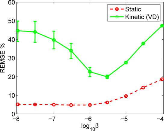
Monte Carlo simulation results demonstrating the benefits of analyzing dynamic reconstruction. While varying the regularization parameter β from 1 × 10⁻⁸ to 3 × 10⁻⁶ has little effect on the REMSE of static ROI quantification, the error in VD (kinetic quantification) can be reduced in half with the optimal regularization parameter.

B. The Proposed Method and Its Relations to Other Work

The above example demonstrates the importance of selecting a proper regularization parameter in PL reconstruction for dynamic PET. Error analysis is essential for proper selection of the regularization parameter. A common method for error analysis is Monte Carlo simulation (such as the one shown in Fig. 1). For example, Monte Carlo simulation was used in [17] to study the error of plasma input function, and in [9] to study the effects of reconstruction parameters, post-reconstruction filtering, and resolution recovery on kinetic parameter estimation. One major disadvantage of Monte Carlo simulation is its high computational cost.

Alternatively, a theoretical approach can be used to analyze noise propagation in parameter estimation. Several methods have been developed for studying resolution and noise properties of static image reconstruction (reconstruction of a single frame), including iteration based methods for the EM algorithm, e.g. [22]-[24], and fixed-point based methods for penalized likelihood reconstruction, e.g. [25]-[31]. Methods for selecting the regularization parameter for lesion detection and ROI quantification have also been developed [32]-[34].

Kinetic parameter estimation requires reconstruction of multiple frames. Thus, the effects of reconstruction methods in dynamic PET are more complicated than in static PET reconstruction. So far, theoretical analysis for kinetic parameter estimation using dynamic PET has been limited. Most existing research on theoretical evaluation of kinetic parameter estimation has considered little of the actual reconstruction effects and treated image reconstruction as unbiased. The noise model for time activity curves was often assumed to be zero mean with variance being proportional to the activity concentration [18]. Under this model, the kinetic parameters estimated using the nonlinear weighted least squares (NLLS) are considered unbiased and the variance is approximated by the inverse of the Fisher information matrix. The computation of the Fisher information matrix can be achieved by either using a numerical perturbation technique, e.g. [1], or a numerical inversion, e.g. [19]. These methods work reasonably well for reconstruction without any regularization, such as filtered backprojection (FBP) with a ramp filter or maximum likelihood (ML) reconstruction. However, as we have shown in Fig. 1, unregularized ML reconstruction may not be the optimal choice for kinetic parameter estimation. This observation has prompted us to study kinetic parameter estimation using the penalized likelihood reconstruction.

This paper aims to develop a theoretical approach to analyzing the effect of penalized likelihood reconstruction on kinetic parameter estimation. PL reconstruction is inherently biased due to the regularization. The bias in the time activity curve will be propagated into the estimated kinetic parameters. In addition, the conventional noise model, which assumes the variance is proportional to the activity, is not valid for PL reconstruction [32]. Here we exploit the accurate noise model that was derived in [34].

By combining the bias and variance of ROI activity quantification with kinetic modeling, we can analyze how regularization in image reconstruction affects kinetic parameter estimation. Approximate expressions for the bias, variance, and ensemble mean squared error of the estimate have been derived, which provide guidance for selecting a proper regularization parameter. Ahn et al. [35] have presented an approximate expression for calculation of the covariance matrix of the kinetic parameters. However, their work is limited to only one-dimensional examples with one tissue compartment model, in which the computation of the sensitivity matrix with respect to kinetic parameters is relatively simple.

The selection of hyperparameter can be also done by other approaches [36]-[40], e.g. the generalized cross validation (GCV), L-curve, and maximum likelihood methods. However, these general approaches are not task-specific and do not guarantee the optimum performance of a clinical task. In addition, most of them require high computational cost. For example it requires evaluations of the MAP solution for different values of hyperparameter to find the corner of the L-curve. In contrast, the theoretical method presented in this paper requires less computation and is specifically aimed to optimize the task of kinetic quantification in dynamic PET.

This paper is organized as follows. Section II presents the theory of PL image reconstruction for dynamic PET and the calculation of the statistics of the TACs. Section III describes the error propagation in kinetic modeling and the calculation of the sensitivity matrix. Validations of the theoretical results using Monte Carlo simulations are given in Section IV. Finally, conclusions are drawn in Section V.

II. Statistical Properties of Time Activity Curves

A. Image Reconstruction for Dynamic PET

PET measurements Y_i, i = 1, . . . , M are well modeled as a collection of independent Poisson random variables,

$$Y_i~\text{Poisson}\left\{{\stackrel{‒}{y}}_i\right\},$$ (1)

with the expectation, $\stackrel{‒}{y}\in I{R}^M$, related to the unknown tracer distribution, $x\in I{R}^N$, through an affine transform

$$\stackrel{‒}{y}=\mathit{Px}+\mathit{r},$$ (2)

where $P\in I{R}^{M\times N}$ is the detection probability matrix with the (i, j)th element being equal to the probability of detecting an event from the jth pixel at the ith measurement, and $r\in I{R}^{M\times 1}$ accounts for the presence of scatter and randoms in the data. The task of image reconstruction is to estimate x from a measurement realization ${\{Y_i=y_i\}}_{i=1}^M$. The log-likelihood function of the Poisson distribution is

$$L(\mathit{y}\mid \mathit{x})=\sum _{i=1}^M{y}_i\log {\stackrel{‒}{y}}_i-{\stackrel{‒}{y}}_i-\log y_i!,$$ (3)

A ML estimate can be found by maximizing (3). However, ML solutions are unstable (i.e., noisy) because the tomography problem is ill-conditioned. Thus, some form of regularization is needed to reconstruct a reasonable image. The penalized maximum likelihood method is to seek the image that maximizes an objective function as follows

$$\widehat{x}=\arg \underset{\mathit{x}\ge 0}{\max }\Phi \left(\mathit{x}\right),\Phi \left(\mathit{x}\right)=L(\mathit{y}\mid \mathit{x})-\beta U\left(\mathit{x}\right),$$ (4)

where U (x) is a roughness penalty included for regularization. The regularization parameter β controls the tradeoff between the resolution and noise. If β is too small, the reconstructed image approaches the ML estimate and becomes very noisy; if β is too large, the reconstructed image becomes very smooth and useful information can be lost.

While various penalty functions have been proposed for image reconstruction, here we focus on the quadratic penalty function. The energy function can then be written as

$$U\left(\mathit{x}\right)=\frac{1}{2}{\mathit{x}}^T\mathit{Rx},$$ (5)

where the superscript “T” denotes vector or matrix transpose, and R is a positive semidefinite matrix.

B. Bias and Variance of Time Activity Curves

The derivation of the bias and variance of the activity inside a ROI has been developed in [34]. For completeness of this paper, we describe the basic derivations here and extend them to TACs.

The average activity inside a ROI at frame $n,{\widehat{\eta }}_n$, can be computed as

$${\widehat{\eta }}_n={\tau }_n{\mathit{f}}_n^T{\widehat{x}}_n,$$ (6)

where ${\widehat{x}}_n$ is the reconstructed image of the integrated radioactivity over the nth time frame duration (in units of Bq·min), f_n is the indicator vector of the ROI at the nth time frame with summation of all elements is 1. In most cases, f_n remains the same for all time frames, but we allow it to be different for different time frames in the analysis. The coefficient τ_n is defined by τ_n = 1/(t_n,e − t_n,s), where t_n,s and t_n,e denote the starting and ending time of time frame n, respectively. If tracer decay is considered in this step, we have τ_n = λ/(e^−λt_n,s – e^−λt_n,e), where λ is the decay constant.

The whole TAC extracted can be denoted by a vector $\widehat{\eta }$ as

$$\widehat{\eta }={\mathcal{D}}_{\tau }{\Omega }^T\widehat{x},$$ (7)

where $\widehat{x}\equiv {\left\{{\widehat{x}}_n\right\}}_{n=1}^{N_f}$ denotes the dynamic images, ${\mathcal{D}}_{\tau }\equiv \mathcal{D}\left[{\tau }_n\right]$ with $\mathcal{D}$ denoting the operation of making diagonal. $\Omega \in I{R}^{N_{f}N\times N_f}$ is the block diagonal matrix composed of ${\left\{{\mathit{f}}_n\right\}}_{n=1}^{N_f}$,

$$\Omega \equiv \mathcal{D}\left[{\mathit{f}}_n\right]=\left(\begin{array}{cccc}\hfill {\mathit{f}}_1\hfill & \hfill \hfill & \hfill \hfill & \hfill \hfill \\ \hfill \hfill & \hfill {\mathit{f}}_2\hfill & \hfill \hfill & \hfill \hfill \\ \hfill \hfill & \hfill \hfill & \hfill \ddots \hfill & \hfill \hfill \\ \hfill \hfill & \hfill \hfill & \hfill \hfill & \hfill {\mathit{f}}_{N_f}\hfill \end{array}\right)$$ (8)

The mean and covariance of the TAC are

$$\mathrm{E}\left[\widehat{\eta }\right]={\mathcal{D}}_{\tau }{\Omega }^T{\mathrm{E}}_{\mathit{y}\mid \mathit{x}}\left[\widehat{x}\left(\mathit{y}\right)\right],$$ (9)

$$\mathrm{cov}\left[\widehat{\eta }\right]={\mathcal{D}}_{\tau }{\Omega }^T{\Sigma }_{\widehat{x}\mid \mathit{x}}\Omega {\mathcal{D}}_{\tau },$$ (10)

where ${\mathrm{E}}_{y\mid x}\left[\widehat{x}\left(y\right)\right]$ and ${\Sigma }_{\widehat{x}\mid x}$ are the mean vector and the covariance matrix of the reconstructed dynamic images for a given tracer distribution $x\equiv {\left\{x_n\right\}}_{n=1}^{N_f}$, respectively.

To proceed, we follow the same approach as in [34] and focus on small ROIs that are surrounded by a large uniform region. Let $x^0\equiv {\left\{x_n^0\right\}}_{n=1}^{N_f}$ denote the reference dynamic image sequence where the activity inside the ROI is equal to the uniform background, and

$${\eta }^0={\mathcal{D}}_{\tau }{\Omega }^T{\mathit{x}}^0$$ (11)

be the TAC of the ROI in the reference dynamic image. Considering the mean of the reconstructed image $\widehat{x}$ as a function of the true tracer distribution x,

$$\mathit{h}\left(\mathit{x}\right)={\mathrm{E}}_{\mathit{y}\mid \mathit{x}}\left[\widehat{x}\left(\mathit{y}\right)\right],$$

we can have the following approximate expression for the mean of the dynamic images

$$\mathit{h}\left(\mathit{x}\right)\approx \mathit{h}\left({\mathit{x}}^0\right)+\nabla \mathit{h}\left({\mathit{x}}^0\right){\mathit{x}}^{\mathrm{ROI}}$$ (12)

where

$${\mathit{x}}^{\mathrm{ROI}}=\mathit{x}-{\mathit{x}}^0,$$

which is the time activity inside the ROI above the background. ▽h(·) is the first derivative matrix of h(·). This derivative matrix can be calculated from the penalized likelihood objective function [25].

Substituting (12) into (9), we obtain an approximate expression for the mean of the ROI TAC

$$\mathrm{E}\left[\widehat{\eta }\right]\approx {\eta }^0+{\mathcal{D}}_{\tau }{\Omega }^T\nabla \mathit{h}\left({\mathit{x}}^0\right){\mathit{x}}^{\mathrm{ROI}}.$$ (13)

Note that here we used the approximation that the reconstruction of the background-only image is unbiased inside the ROI, i.e.

$${\Omega }^T\mathit{h}\left({\mathit{x}}^0\right)\approx {\Omega }^T{\mathit{x}}^0.$$

This approximation is reasonable when the background region is relatively smooth, as we will demonstrate in the computer simulations.

Define

$$\eta ={\mathcal{D}}_{\tau }{\Omega }^T\mathit{x}$$

as the true TAC of the ROI. Subtracting η⁰ from both sides of (13) yields the bias of the TAC

$$\begin{array}{cc}\hfill \mathrm{bias}\left[\widehat{\eta }\right]& =\mathrm{E}\left[\widehat{\eta }\right]-\eta \hfill \\ \hfill & \approx {\mathcal{D}}_{\tau }{\Omega }^T(\nabla \mathit{h}\left({\mathit{x}}^0\right)-\mathit{I}){\mathit{x}}^{\mathrm{ROI}},\hfill \end{array}$$ (14)

where I is the identity matrix.

In this paper we use the frame-by-frame reconstruction model which does not include any temporal correlation, so the matrices ▽h(·) and ${\Sigma }_{\widehat{x}\mid x}$ are block diagonal,

$$\nabla \mathit{h}\left({\mathit{x}}^0\right)=\mathcal{D}\left[\nabla {\mathit{h}}_n\left({\mathit{x}}_n^0\right)\right],$$ (15)

$${\Sigma }_{\widehat{x}\mid \mathit{x}}=\mathcal{D}\left[{\Sigma }_{{\widehat{x}}_n\mid {\mathit{x}}_n}\right],$$ (16)

where $\nabla h_n\left(x_n^0\right)$ and ${\Sigma }_{{\widehat{x}}_n\mid x_n}$ are the resolution matrix and the covariance matrix of the reconstructed image of the nth time frame, respectively. They can be computed by

$${\nabla h}_n\left({\mathit{x}}_n^0\right)={[{\mathit{F}}_n+{\beta }_n\mathit{R}]}^{-1}{\mathit{F}}_n,$$ (17)

$${\Sigma }_{{\widehat{x}}_n\mid {\mathit{x}}_n}\approx {[{\mathit{F}}_n+{\beta }_n\mathit{R}]}^{-1}{\mathit{F}}_n{[{\mathit{F}}_n+{\beta }_n\mathit{R}]}^{-1},$$ (18)

where $F_n=P^T\mathcal{D}[1∕{\left({\stackrel{‒}{y}}_n\right)}_i]P$ is the Fisher information matrix for time frame n and β_n is the regularization parameter for time frame n. Readers are referred to [26], [29], [34] for details.

Substituting (17) and (18) into (14) and (10) yields the following approximate expressions of the bias and variance of the TAC

$$\mathrm{bias}\left[{\widehat{\eta }}_n\right]\approx -{\beta }_n{\tau }_n{\mathit{f}}_n^T{[{\mathit{F}}_n+{\beta }_n\mathit{R}]}^{-1}{\mathit{Rx}}_n^{\mathrm{ROI}},$$ (19)

$$\mathrm{var}\left[{\widehat{\eta }}_n\right]\approx {\tau }_n^2{\mathit{f}}_n^T{[{\mathit{F}}_n+{\beta }_n\mathit{R}]}^{-1}{\mathit{F}}_n{[{\mathit{F}}_n+{\beta }_n\mathit{R}]}^{-1}{\mathit{f}}_n.$$ (20)

C. Efficient Calculation

The computation of the bias and variance involve the inverse of [F_n + β_nR]. Direct calculation is very time-consuming due to the large size of the matrix (number of image pixels by number of image pixels), so we use block circulant matrices F_n(j) and R(j) that are constructed using the jth columns of F_n and R, respectively, to approximate F_n and R locally as proposed in [29]. We thus have the following approximations for the bias and covariance,

$$\mathrm{bias}\left[{\widehat{\eta }}_n\right]\approx -{\beta }_n{\tau }_n{\mathit{f}}_n^T{\left[{\mathit{H}}_n\left(j\right)\right]}^{-1}\mathit{R}\left(j\right){\mathit{x}}_n^{\mathrm{ROI}},$$ (21)

$$\mathrm{var}\left[{\widehat{\eta }}_n\right]\approx {\tau }_n^2{\mathit{f}}_n^T{\left[{\mathit{H}}_n\left(j\right)\right]}^{-1}{\mathit{F}}_n\left(j\right){\left[{\mathit{H}}_n\left(j\right)\right]}^{-1}{\mathit{f}}_n,$$ (22)

where H_n(j) = F_n(j) + β_nR(j) and j is the index of the voxel at the center of the ROI.

The constructed circulant matrices can be diagonalized by the Fourier transform,

$${\mathit{F}}_n\left(j\right)={\mathit{Q}}^T\mathrm{diag}\left[{\lambda }_{ni}\left(j\right)\right]\mathit{Q},$$

$$\mathit{R}\left(j\right)={\mathit{Q}}^T\mathrm{diag}\left[{\mu }_i\left(j\right)\right]\mathit{Q},$$

$${\left[{\mathit{H}}_n\left(j\right)\right]}^{-1}={\mathit{Q}}^T{\mathrm{diag}}^{-1}[{\lambda }_{ni}\left(j\right)+{\beta }_n{\mu }_i\left(j\right)]\mathit{Q},$$

where {λ_ni(j), i = 1, · · · , N} are the Fourier coefficients (or eigenvalues) of F_n(j) and {μ_i(j), i = 1, · · · , N} are the Fourier coefficients of R(j)¹. $Q\in I{R}^{N\times N}$ and Q^T represent the Kronecker form of the Fourier transform and its inverse, respectively.

Substituting these circulant matrix approximations into (21) and (22), we can obtain the following expressions

$$\begin{array}{cc}\hfill \mathrm{bias}\left[{\widehat{\eta }}_n\right]& \approx -{\beta }_n{\tau }_n{\mathit{f}}_n^T{\mathit{Q}}^T\mathrm{diag}\left[\frac{{\mu }_i\left(j\right)}{{\lambda }_{ni}\left(j\right)+{\beta }_n{\mu }_i\left(j\right)}\right]{\mathit{Qx}}_n^{\mathrm{ROI}}\hfill \\ \hfill & \approx -{\beta }_n{\tau }_n\sum _i\frac{{\mu }_i\left(j\right){\xi }_{ni}^{\ast }{\zeta }_{ni}}{{\lambda }_{ni}\left(j\right)+{\beta }_n{\mu }_i\left(j\right)},\hfill \end{array}$$ (23)

and

$$\begin{array}{cc}\hfill \mathrm{var}\left[{\widehat{\eta }}_n\right]& \approx {\tau }_n^2{\mathit{f}}_n^T{\mathit{Q}}^T\mathrm{diag}\left[\frac{{\lambda }_{ni}\left(j\right)}{{[{\lambda }_{ni}\left(j\right)+{\beta }_n{\mu }_i\left(j\right)]}^2}\right]{\mathit{Qf}}_n\hfill \\ \hfill & \approx {\tau }_n^2\sum _i\frac{{\lambda }_{ni}\left(j\right){\mid {\xi }_{ni}\mid }^2}{{[{\lambda }_{ni}\left(j\right)+{\beta }_n{\mu }_i\left(j\right)]}^2},\hfill \end{array}$$ (24)

where {ξ_ni, i = 1, · · · , N} and {ζ_ni, i = 1, · · · , N} are the Fourier transforms of f_n and x_n^ROI, respectively, and ‘*’ denotes complex conjugate.

III. Error Propagation in Kinetic Parameter Estimation

A. Tracer Kinetic Modeling

Tracer kinetic behaviors in dynamic PET imaging are often described by compartmental models which mathematically can be represented by a set of ordinary differential equations,

$$\frac{\mathrm{d}}{\mathrm{d}t}\mathit{c}\left(t\right)=\mathit{Kc}\left(t\right)+\mathit{Lu}\left(t\right)$$ (25)

where c(t) is a column vector representing the activity concentration of different tissue compartments at time t, K and L are the kinetic parameter matrices which are comprised of various rate constants, and u(t) denotes the system input.

For a commonly used three-compartment model, $c\left(t\right)=\left(\begin{array}{c}\hfill C_{\mathrm{f}}\left(t\right)\hfill \\ \hfill C_{\mathrm{b}}\left(t\right)\hfill \end{array}\right)$, where C_f(t) and C_b(t) are the concentrations in the free and bound compartments; $u\left(t\right)=\left(\begin{array}{c}\hfill C_{\mathrm{P}}\left(t\right)\hfill \\ \hfill 0\hfill \end{array}\right)$ where C_p(t) is the concentration in the plasma; $K=\left(\begin{array}{cc}\hfill -(k_2+k_3)\hfill & \hfill k_4\hfill \\ \hfill k_3\hfill & \hfill -k_4\hfill \end{array}\right)$, $L=\left(\begin{array}{cc}\hfill K_1\hfill & \hfill 0\hfill \\ \hfill 0\hfill & \hfill 0\hfill \end{array}\right)$, where K₁, k₂, k₃, k₄ are the tracer rate constants. The differential equation model (25) can be analytically solved by using the Laplace transform and the solution is

$$\mathit{c}\left(t\right)=\mathit{q}\left(t\right)\otimes C_{\mathrm{p}}\left(t\right)$$ (26)

where the impulse response function matrix q(t) is given by

$$\mathit{q}\left(t\right)=\frac{K_1}{\Delta \alpha }\left(\begin{array}{cc}\hfill k_4-{\alpha }_1\hfill & \hfill {\alpha }_2-k_4\hfill \\ \hfill k_3\hfill & \hfill -k_3\hfill \end{array}\right)e^{-\alpha \left(t\right)},$$ (27)

$‘‘\otimes ’’$ denotes the convolution operation, Δα = α₂ – α₁ with ${\alpha }_{1,2}=\frac{1}{2}(k_2+k_3+k_4)\mp \frac{1}{2}{[{(k_2+k_3+k_4)}^2-4k_2{k}_4]}^{1∕2}$, and $e^{-\alpha \left(t\right)}={\left(e^{-{\alpha }_{1}t},e^{-{\alpha }_{2}t}\right)}^T$.

Note that c(t) is unmeasurable. The quantity that PET measures is the total activity concentration

$$C_{\mathrm{T}}\left(t\right)=(1-f_v)1^T\mathit{c}\left(t\right)+f_v{\mathit{C}}_{wb}\left(t\right),$$ (28)

where 1 is the all-one vector and f_v is the fractional volume which represents the fraction of whole blood in the region of interest. C_wb(t) is the activity concentration in whole blood. In practice, PET data are binned into discrete time frames. With consideration of tracer decay, the measured quantity in time frame n is

$$C_{\mathrm{T}}\left(n\right)=\frac{1}{\Delta t_n}{\int }_{t_{n,s}}^{t_{n,e}}{C}_T\left(\tau \right)e^{-\lambda \tau }\mathrm{d}\tau ,$$ (29)

where Δt_n = t_n,e – t_n,s. An estimate of C_T(n) is obtained using (7). Note that we use C_T(n) to represent the time integral of the activity and C_T(t) or C_T(τ) to represent the continuous-time activity.

Given a measured TAC, $\{{\widehat{\eta }}_n,n=1,\cdots ,N_f\}$, the task of kinetic analysis is to estimate the rate constants in K and L, and f_v, which is usually accomplished by using a nonlinear least squares formulation as follows

$$\widehat{\kappa }=\arg \underset{\kappa }{\min }\Phi (\widehat{\eta }\mid \kappa ),$$ (30)

$$\Phi (\widehat{\eta }\mid \kappa )=\sum _{n=1}^N{w}_n{\left({\widehat{\eta }}_n-C_{\mathrm{T}}(n;\kappa )\right)}^2,$$ (31)

where {w_n} are the weights and k are the kinetic parameters. For the three-compartment model, k = [K₁, k₂, k₃, k₄, f_v]^T.

B. Error Propagation into Microparameters

The estimated kinetic parameters $\widehat{\kappa }$ can be represented as a function of the TAC measurement $\widehat{\eta }$,

$$\widehat{\kappa }=\mathit{g}\left(\widehat{\eta }\right).$$ (32)

Using the first-order Taylor expansion, we have

$$\widehat{\kappa }\approx \mathit{g}\left(\eta \right)+\nabla \mathit{g}\left(\eta \right)(\widehat{\eta }-\eta ),$$ (33)

where n denotes the actual TAC that is defined in (29), ▽g(·) is the first-order derivative of g(·) and can be found by using the fixed point condition

$${\phantom{\mid }\frac{\partial \Phi (\eta \mid \kappa )}{\partial \kappa }\mid }_{\kappa =\mathit{g}\left(\eta \right)}=0.$$ (34)

Taking the derivative with respect to n and using the chain rule [25], we get the following for the least squares objective function:

$$\nabla \mathit{g}\left(\eta \right)={\left[{\mathit{S}}^T\mathit{WS}\right]}^{-1}{\mathit{S}}^T\mathit{W},$$ (35)

where S is the sensitivity matrix whose (n, l)th element is $\frac{\partial C_{\mathrm{T}}\left(n\right)}{\partial {\kappa }_l}$, n = 1, · · ·, N_f; l = 1, · · · , N_p with N_p being the number of unknown parameters to be estimated and W is the diagonal matrix whose nth diagonal element is w_n.

Thus the mean of the estimate $\widehat{\kappa }$ can be approximated by

$$\mathrm{E}\left[\widehat{\kappa }\right]\approx \mathit{g}\left(\eta \right)+\nabla \mathit{g}\left(\eta \right)(\mathrm{E}\left[\widehat{\eta }\right]-\eta ),$$ (36)

and the bias is

$$\begin{array}{cc}\hfill \mathrm{bias}\left[\widehat{\kappa }\right]& =\mathrm{E}\left[\widehat{\kappa }\right]-\kappa \hfill \\ \hfill & \approx \nabla \mathit{g}\left(\eta \right)(\mathrm{E}\left[\widehat{\eta }\right]-\eta )\hfill \\ \hfill & \approx {\left[{\mathit{S}}^T\mathit{WS}\right]}^{-1}{\mathit{S}}^T\mathit{W}\mathrm{bias}\left[\widehat{\eta }\right].\hfill \end{array}$$ (37)

In the above derivation, we have assumed that the kinetic parameters estimated from the noise free TAC are unbiased, i.e. k = g(n).

From (33), the covariance of the estimate $\widehat{\kappa }$ is

$$\begin{array}{cc}\hfill \mathrm{cov}\left[\widehat{\kappa }\right]& \approx \nabla \mathit{g}\left(\eta \right)\mathrm{cov}\left[\widehat{\eta }\right]{[\nabla \mathit{g}\left(\eta \right)]}^T\hfill \\ \hfill & \approx {\left[{\mathit{S}}^T\mathit{WS}\right]}^{-1}{\mathit{S}}^T\mathit{W}\mathrm{cov}\left[\widehat{\eta }\right]\mathit{WS}{\left[{\mathit{S}}^T\mathit{WS}\right]}^{-1}\hfill \end{array}$$ (38)

where cov[$\widehat{\eta }$] = diag(var[${\widehat{\eta }}_n$]) and var[${\widehat{\eta }}_n$] is the variance of ${\widehat{\eta }}_n$ given in (20) and can be computed by (24).

If we set W as

$$\mathit{W}={\mathrm{diag}}^{-1}\left(\mathrm{var}\left[{\widehat{\eta }}_n\right]\right),$$ (39)

cov[$\widehat{\kappa }$] can be simplified to

$$\mathrm{cov}\left[\widehat{\kappa }\right]\approx {\left[{\mathit{S}}^T{\mathrm{diag}}^{-1}\left(\mathrm{var}\left[{\widehat{\eta }}_n\right]\right)\mathbf{S}\right]}^{-1}.$$ (40)

C. Calculation of the Sensitivity Matrix

The above derivation shows that the bias and variance of the estimated kinetic parameters are related to the bias and variance of the TAC through the sensitivity matrix S, of which the (n, l)th element is the derivative of the TAC value in the nth time frame, C_T(n), with respect to the lth kinetic parameter in k.

From (28), we have

$$\frac{\partial C_{\mathrm{T}}\left(t\right)}{\partial f_v}=-1^T\mathit{c}\left(t\right)+{\mathit{C}}_{wb}\left(t\right),$$ (41)

and

$$\frac{\partial C_{\mathrm{T}}\left(t\right)}{\partial k_l}=(1-f_v)1^T\frac{\partial \mathit{c}\left(t\right)}{\partial k_l},l=1,\cdots ,L-1.$$ (42)

Direct calculation of $\frac{\partial c\left(t\right)}{\partial {\kappa }_l}$ using (26) is tedious and cannot be extended to higher-order compartmental models. Here we present an easier and more general approach.

We start from (25) and take the derivative with respect to

$$\frac{\mathrm{d}}{\mathrm{d}t}\frac{\partial \mathit{c}\left(t\right)}{\partial {\kappa }_l}=\mathit{K}\frac{\partial \mathit{c}\left(t\right)}{\partial {\kappa }_l}+{\mathit{u}}^l\left(t\right).$$ (43)

The new input u^l(t) in the above ordinary differential equation is given by

$${\mathit{u}}^l\left(t\right)=\frac{\partial \mathit{K}}{\partial {\kappa }_l}\mathit{c}\left(t\right)+\frac{\partial \mathit{L}}{\partial {\kappa }_l}\mathit{u}\left(t\right).$$ (44)

For the three-compartment model, we have

$${\mathit{u}}^1\left(t\right)=\left(\begin{array}{c}\hfill 1\hfill \\ \hfill 0\hfill \end{array}\right)C_{\mathrm{P}}\left(t\right),{\mathit{u}}^2\left(t\right)=\left(\begin{array}{c}\hfill -1\hfill \\ \hfill 0\hfill \end{array}\right)C_{\mathrm{f}}\left(t\right),$$

$${\mathit{u}}^3\left(t\right)=\left(\begin{array}{c}\hfill -1\hfill \\ \hfill 1\hfill \end{array}\right)C_{\mathrm{f}}\left(t\right),{\mathit{u}}^4\left(t\right)=\left(\begin{array}{c}\hfill 1\hfill \\ \hfill -1\hfill \end{array}\right)C_{\mathrm{b}}\left(t\right).$$

Once u^l(t) is given, we can solve (43) using the Laplace transform. The solutions for the three-compartment model are

$$\frac{\partial \mathit{c}\left(t\right)}{\partial {\kappa }_1}={\mathit{q}}_1\left(t\right)\otimes C_{\mathrm{P}}\left(t\right),$$ (45)

$$\frac{\partial \mathit{c}\left(t\right)}{\partial {\kappa }_2}=-{\mathit{q}}_1\left(t\right)\otimes C_{\mathrm{f}}\left(t\right),$$ (46)

$$\frac{\partial \mathit{c}\left(t\right)}{\partial {\kappa }_3}={\mathit{q}}_2\left(t\right)\otimes C_{\mathrm{f}}\left(t\right),$$ (47)

$$\frac{\partial \mathit{c}\left(t\right)}{\partial {\kappa }_4}=-{\mathit{q}}_2\left(t\right)\otimes C_{\mathrm{b}}\left(t\right),$$ (48)

where

$${\mathit{q}}_1\left(t\right)=\frac{1}{\Delta \alpha }\left(\begin{array}{cc}\hfill k_4-{\alpha }_1\hfill & \hfill {\alpha }_2-k_4\hfill \\ \hfill k_3\hfill & \hfill -k_3\hfill \end{array}\right)e^{-\alpha \left(t\right)}$$

and

$${\mathit{q}}_2\left(t\right)=\frac{1}{\Delta \alpha }\left(\begin{array}{cc}\hfill {\alpha }_1\hfill & \hfill -{\alpha }_2\hfill \\ \hfill {\alpha }_2-(k_3+k_4)\hfill & \hfill (k_3+k_4)-{\alpha }_1\hfill \end{array}\right)e^{-\alpha \left(t\right)}.$$

The (n, l)th element of the sensitivity matrix S is finally evaluated by

$$s_{nl}=\frac{\partial C_{\mathrm{T}}\left(n\right)}{\partial {\kappa }_l}=\frac{1}{t_{n,e}-t_{n,s}}{\int }_{t_{n,s}}^{t_{n,e}}\frac{\partial C_{\mathrm{T}}\left(\tau \right)}{\partial {\kappa }_l}{e}^{-\lambda \tau }\mathrm{d}\tau ,$$ (49)

where $\frac{\partial C_{\mathrm{T}}\left(\tau \right)}{\partial {\kappa }_l}$ is given in (41) and (42).

D. Error Propagation into Macroparameters

The kinetic parameters k are referred to as microparameters. The parameters of biomedical interest are called macroparameters, which are functions of the microparameters. Examples of the macroparameters that are commonly used include the influx constant (KI) in metabolic studies, and the volume of distribution (VD) and binding potential (BP) in neuroreceptor studies. They are related to the microparameters in the three-compartment model by the following equations:

$$KI=\frac{K_1{k}_3}{k_2+k_3},$$ (50)

$$VD=\frac{K_1}{k_2}\left(1+\frac{k_3}{k_4}\right),$$ (51)

$$BP=\frac{k_3}{k_4}.$$ (52)

Using the first-order Taylor series approximation, we can approximate the bias and variance of a macroparameter ψ(k) by

$$\mathrm{bias}\left[\psi \right]\approx {\nabla }_{\kappa }\psi \mathrm{bias}\left[\widehat{\kappa }\right],$$ (53)

$$\mathrm{var}\left[\psi \right]\approx {\nabla }_{\kappa }{\psi }^T\mathrm{cov}\left[\widehat{\kappa }\right]{\nabla }_{\kappa }\psi ,$$ (54)

where △_kψ denotes the derivatives of the macroparameter with respect to microparameters. For the macroparameters shown above, △_kψ's are given by

$${\nabla }_{\kappa }KI={\left(\frac{KI}{K_1}-\frac{KI}{k_2+k_3}\frac{KI{k}_2}{k_3(k_2+k_3)}0\right)}^T,$$ (55)

$${\nabla }_{\kappa }VD={\left(\frac{VD}{K_1}-\frac{VD}{k_2}\frac{K_1}{k_2{k}_4}-\frac{K_1{k}_3}{k_2{k}_4^2}\right)}^T,$$ (56)

$${\nabla }_{\kappa }BP={(00\frac{1}{k_4}-\frac{BP}{k_4})}^T.$$ (57)

One figure of merit that is often used to assess the quality of parameter estimation is the ensemble mean squared error, which is equal to the sum of the squared bias and the variance

$$\mathrm{EMSE}\left[\psi \right]=\mathrm{bias}{\left[\psi \right]}^2+\mathrm{var}\left[\psi \right].$$ (58)

The above theoretical expressions of the bias and variance can be used to calculate the EMSE as a function of the regularization parameter. A user can then select the regularization parameter that results in the minimum EMSE. Of course, other figures of merit that weight bias and variance differently can also be used. We use EMSE as an example in this paper because of its simplicity.

IV. Computer Simulations

A. Validation of the Theoretical Expressions

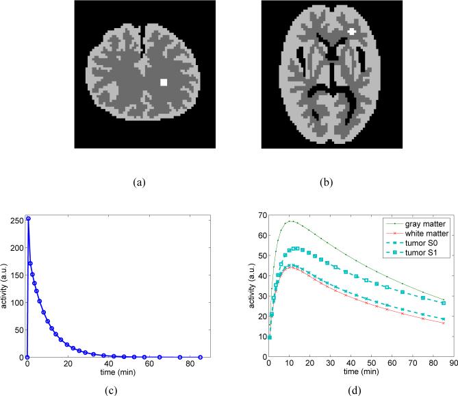
We conducted computer simulations to validate the theoretical expressions. We simulated two brain phantoms (Fig. 2(a) and (b)). A small tumor was inserted in the white matter region in each phantom. The TAC of each region was generated using a three-compartment model with an analytical blood input function [41] and with the kinetic parameters taken from literature [42]. The kinetic parameters used were: K₁ = 0.1104 mL/min/mL, k₂ = 0.1910 min⁻¹, k₃ = 0.1024 min⁻1, and k₄ = 0.0094 min⁻¹ for the gray matter region; K₁ = 0.0622 mL/min/mL, k₂ = 0.1248 min⁻¹, k₃ = 0.0700 min⁻¹, and k₄ = 0.0097 min⁻¹ for the white matter region; and K₁ = 0.0640 mL/min/mL, k₂ = 0.1272 min⁻¹, k₃ = 0.0738 min⁻¹, k₄ = 0.0081 min⁻¹ for the tumor (referred to as ‘tumor S0’). We also simulated a different case of tumor kinetics (referred to as ‘tumor S1’) with K₁ = 0.0640 mL/min/mL, k₂ = 0.08904 min⁻¹, k₃ = 0.0738 min⁻¹, k₄ = 0.00567 min⁻¹, which has a larger difference in TAC from the white matter. In all the simulations, f_v was set to zero. The scanning sequence consists of 24 time frames: 5 frames of 60 seconds, 5 frames of 120 seconds, 5 frames of 180 seconds, 5 frames of 250 seconds and 3 frames of 600 seconds.

Fig. 2.

Simulation settings. (a) and (b): two brain phantoms consist of gray matter, white matter and a small tumor inside the white matter; (c) the blood input function; and (d) the regional time activity curves.

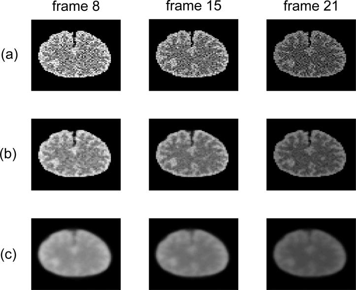
The blood input and the regional TACs are shown in Fig. 2. These TACs were integrated for each time frame and forward projected to form dynamic sinograms. Poisson noise was then generated, which resulted in a total number of events over the 90 minutes equal to 50M. One hundred independent identically distributed data sets were generated and reconstructed frame-by-frame using the penalized likelihood method and the preconditioned conjugate gradient (PCG) algorithm. The PCG was run for 100 iterations for each β value to guarantee convergence. The regularization parameter β in the PL reconstruction was selected for the last frame and was scaled for the earlier frames with respect to their total counts. The β values vary from 1 × 10⁻⁸ to 1 × 10⁻⁴, which covers a reasonable range from very noisy images to oversmooth images. Fig. 3 shows the reconstructed images of a noisy dataset.

Fig. 3.

Reconstructed dynamic images of one noisy data set with different regularization parameters. Columns from left to right correspond to different time frames number 8, 15 and 21; rows from top to bottom correspond to (a) β = 10⁻⁸, (b) β = 3 × 10⁻⁶, and (c) β = 10⁻⁴.

We selected the tumor region as the ROI. TACs were extracted from the reconstructed images and the kinetic parameters were estimated by using the nonlinear least squares method with the Levenberg-Marquardt algorithm. The weighting factor was chosen as being inversely proportional to the variance of the TAC that was estimated from 100 Monte Carlo realizations. Figure 4 shows the bias and variance of the estimated TAC of tumor S1 in the first phantom (Fig. 2(a)) with different regularization parameters, computed by both the theoretical expressions and the Monte Carlo methods. We can see that when we increase the β value, the bias is increased, but the variance is reduced. The staircase shape in the variance plot is a result of the change in time frame duration. The relative REMSE in Fig. 4(c) was calculated as $\sqrt{{\sum }_n\Delta t_n\mathrm{E}\left[{({\widehat{\eta }}_n-{\eta }_n)}^2\right]}∕\sqrt{{\sum }_n\Delta t_n{\eta }_n^2}\times 100\%$. In general the theoretical predictions match the Monte Carlo results very well.

Fig. 4.

Bias, variance, and REMSE of the estimated time activity curve of tumor S1 using the theoretical prediction and Monte Carlo method with different regularization parameters.

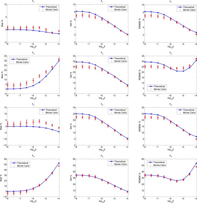
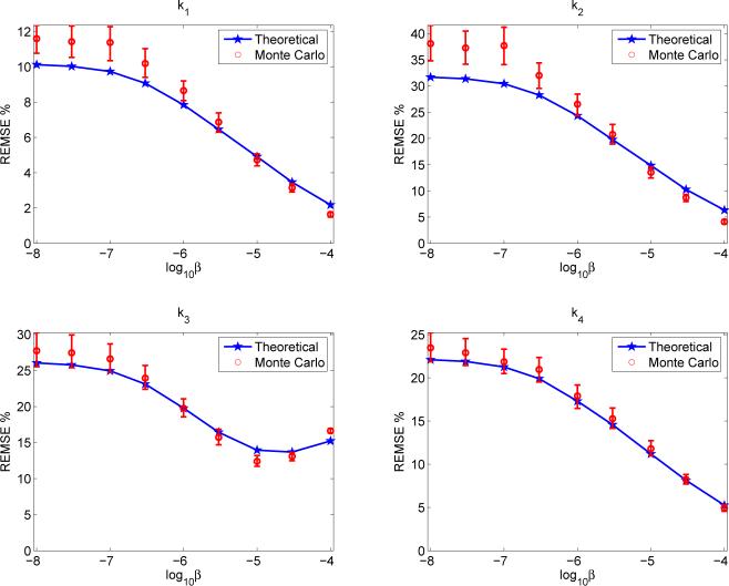
Figure 5 shows the bias, variance, and REMSE of the estimated microparameters, K₁, k₂, k₃, k₄, of tumor S1 in the first phantom. It is interesting to note that regularization has different effects on different parameters. For example, the biases of K₁ and k₃ are insensitive to the change of the regularization parameter, whereas the biases of k₂ and k₄ increase dramatically as the regularization parameter increases. For all parameters, the variance decreases as the regularization parameter increases. As a result, the REMSE is a monotonically decreasing function of the regularization parameter for K₁ and k₃, but exhibits a minimum at a midrange regularization for k₂ and k₄. The theoretical results match the Monte Carlo results reasonably well.

Fig. 5.

Predictions of the bias, standard deviation and EMSE of microparameters (K₁, k₂, k₃, k₄) of tumor S1 in the first phantom (Fig. 2(a)) by the theoretical method and Monte Carlo method.

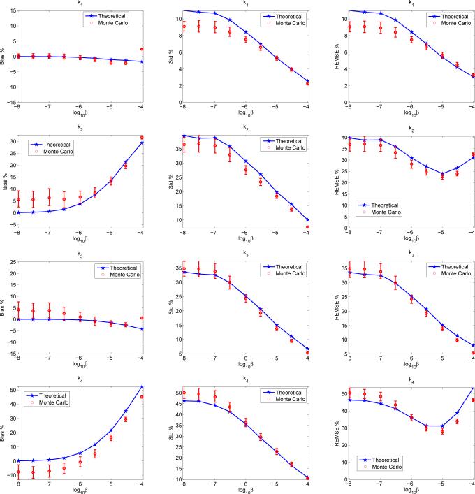
The results of the second phantom are plotted in Fig. 6, which also shows good match between the theoretical predictions and the Monte Carlo results. The trend of each plot is quite similar to that shown in Fig. 5. Given the similarity between the results of the two phantoms, we will focus on the first phantom in the rest of the Section.

Fig. 6.

Predictions of the bias, standard deviation and EMSE of microparameters ((K₁, k₂, k₃, k₄) of tumor S1 in the second phantom (Fig. 2(b)) by the theoretical method and Monte Carlo method.

The different trends in the bias curves of the four microparameters arise because in this simulation K₁ and k₃ of the tumor region were similar to those of the surrounding white matter and, hence, are insensitive to regularization; whereas k₂ and k₄ of the tumor are different from those of the white matter and, hence, are sensitive to regularization. To validate this hypothesis, we performed four more sets of simulations, in which we kept all the kinetic parameters, except one, of the tumor to be the same as those of the surrounding white matter. The kinetic parameter being studied in each simulation is set to be 30% greater than that of the white matter. Figure 7 shows the RMSE curves of the four parameters when the tumor kinetics is generated with a 30% increase in k₃. It shows that the errors of all the other kinetic parameters monotonically reduce as the regularization parameter increases while the error of k₃ achieves a minimum with a medium regularization. The results of the other three sets of simulation are similar, although the values of the optimum regularization parameter are different for different kinetic parameters (they are 1 × 10⁻⁶, 1 × 10⁻⁵, 1 × 10⁻⁵, 1 × 10⁻⁵ for K₁, k₂, k₃, k₄, respectively). These results demonstrate the importance of using a task-specific figure of merit when selecting reconstruction parameters.

Fig. 7.

Effects of regularization on kinetic parameter estimation. The tumor kinetics was generated using the same kinetic parameters as the background white matter except a 30% increase in k₃.

It is also noted that Monte Carlo results (K₁, k₂, k₃, and k₄) are biased even with very small β values. Using computer-generated Gaussian distributed TACs, we found that the bias is intrinsic to the nonlinear least squares fitting when the noise is high, which is the case with small β values. Similar results have also been reported in [43].

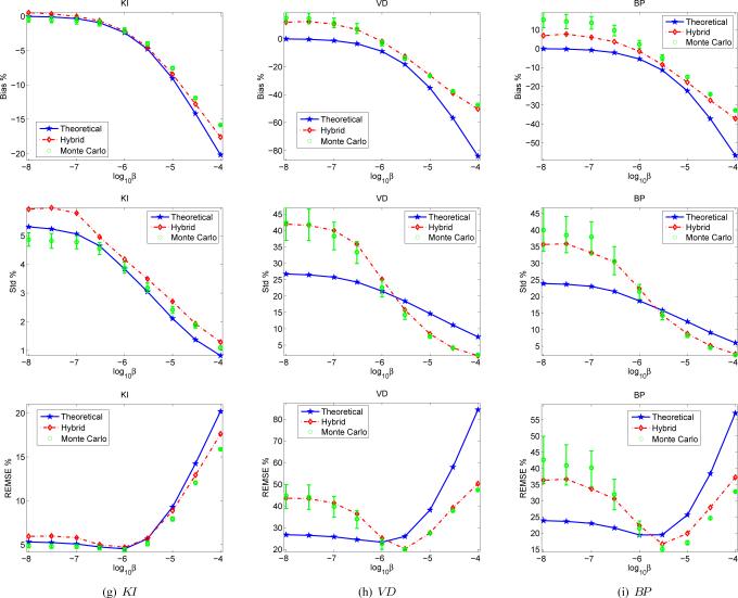
Figure 8 compares the bias, variance, and ensemble mean squared errors for the estimated macroparameters. The theoretical prediction matches with the Monte Carlo results very well for KI. At small β values, the theoretical prediction underestimates the EMSE of VD and BP, but overestimates the EMSE of VD and BP at large β values.

Fig. 8.

Comparison of the theorectial prediction and Monte Carlo method for estimating REMSE of (a) KI, (b) VD, and (c) BP for tumor S1 with different regularization parameters.

B. Improved Prediction Using a Hybrid Method

The error in the theoretical method is due to the nonlinearity in the transformation between the microparameters and the macro-parameters. To solve this problem, we propose a hybrid approach. After computing the bias and covariance of the microparameters by using the theoretical expressions, we calculate an ensemble of the macroparameters from an ensemble of computer-generated Monte Carlo samples of the microparameters by assuming they follow a multivariate Gaussian distribution with the estimated mean and covariance. The bias and variance of the macroparameters are then calculated from the ensemble. The bias, variance, and EMSE of VD and BP are predicted very well by the hybrid approach as compared with the Monte Carlo results as shown in Fig. 8.

Note that the use of the hybrid method does not increase the computation time because the transformations from the microparameters to the macroparameters are simple and easy to calculate. In this paper, 10,000 Monte Carlo samples were used, which took less than 1 second in MATLAB on a 2 GHz PC. Thus, the computation cost for the hybrid method is the same as that of the fully theoretical method and can still be several orders of magnitude faster than the Monte Carlo method for the same accuracy.

C. Effect of Count Levels

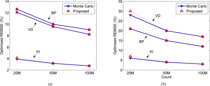
We also simulated different count levels. The minimum REMSE predicted by the proposed method and Monte Carlo method are shown as functions of count level in Fig. 9. As expected, the minimum REMSE decreases as the count level increases. For all the three macroparameters, the results of the proposed method (hybrid approach) match well with the Monte Carlo results. Note that the reduction in REMSE is less than the reduction in variance as predicted from the count level because bias is independent of count level. We also compared the regularization parameter selected by the Monte Carlo method and the theoretical prediction for achieving the minimum REMSE. The results are shown in Table I. In all cases, the optimum regularization parameters predicted by the proposed method are very close to the Monte Carlo results. We note that when the count level is very low, the first-order approximation employed in this paper becomes less accurate to predict the noise propagation in the nonlinear least squares fitting.

Fig. 9.

The predicted minimum REMSE of the macroparameters under different count levels by the hybrid approach and the Monte Carlo approach. (a) Tumor S0 and (b) tumor S1.

TABLE I.

Optimum regularization parameter log₁₀ β chosen by the Monte Carlo and the proposed methods (in parentheses)

SO, Count(M)	KI	VD	BP
20	−4.0 (−3.5)	−4.0 (−4.0)	−4.0 (−4.0)
50	−4.5 (−4.5)	−5.0 (−5.0)	−5.0 (−5.0)
100	−5.0 (−5.0)	−5.5 (−5.5)	−5.5 (−5.5)

SI, Count(M)	KI	VD	BP
20	−6.0 (−5.5)	−5.0 (−4.5)	−4.5 (−4.5)
50	−6.0 (−6.0)	−5.5 (−5.5)	−5.5 (−5.5)
100	−6.5 (−6.5)	−6.0 (−6.0)	−6.0 (−6.0)

D. Practical Considerations

1) “Plug-in” Method

A critical problem with using the above theoretical method is that it requires the true value of the TAC inside the ROI (or equivalently the kinetic parameters) to calculate the bias of the TAC. This can be circumvented by using the following “plug-in” strategy. For a given dataset, we first reconstruct the images with a small regularization parameter to get the TAC and estimate the kinetic parameters of the ROI. We can then “plug-in” the resulting kinetic parameters and the fitted TAC into the theoretical expressions as the “true” value to estimate the optimal regularization parameter.

The performance of the plug-in method is demonstrated in Fig. 10 where we show the resulting REMSE of the FDG data set when we reconstruct each noisy data set using the regularization parameter selected by the “plug-in” strategy. The resulting REMSE is close to the minimum REMSE value obtained with the optimal β selected using the noise-free TAC, indicating that the “plug-in” method is very effective.

Fig. 10.

The effect of the “plug-in” method and ROI delineation on the selection of the regularization parameter.

2) Effect of ROI Definition

Another practical issue is the definition of the ROI. In the above simulation, we use the true tumor region as the ROI. However, in real situations, the ROI delineation will not be exact. To investigate the effects of imperfect ROI on the plug-in approach, we repeated the above plug-in method using both an enlarged ROI (+45%) and a shrunk ROI (−45%). The results are also shown in Fig. 10. It shows that imperfect ROI increase the REMSE slightly compared with the exact ROI, but results are acceptable, in particular for VD and BP. These results demonstrate that the proposed method is robust enough for practical applications.

V. Conclusions

Analysis of PL image reconstruction shows that proper selection of the regularization parameters is important for dynamic PET. To explore the potential of PL reconstruction for dynamic PET, we have developed a theoretical approach to analyzing penalized likelihood image reconstruction for quantification of kinetic parameters. We performed an analytical study of the noise propagation from raw PET measurement into kinetic modeling. Approximate expressions of the bias, variance and ensemble mean squared error of the kinetic parameters have been derived as a function of the regularization parameter in the PL reconstruction. Computer simulations show that the theoretical predictions match well with the Monte Carlo results. A plug-in method has also been developed and validated for applying the theoretical results to guide the selection of the regularization parameter in the PL reconstruction for dynamic PET. While we used EMSE to select the regularization parameter, we should point out that the proper figure of merit is task dependent and the proposed method is applicable to other figures of merit that are functions of the bias and variance. The analysis can also be extended to dynamic PET reconstruction that uses smooth temporal basis functions by properly modeling the correlation between the basis functions.

References

- 1.Mazoyer BM, Huesman RH, Budinger TF, Knittel BL. Dynamic PET data-analysis. Journal of Computer Assisted Tomography. 1986;10(4):645–653. doi: 10.1097/00004728-198607000-00020. [DOI] [PubMed] [Google Scholar]
- 2.Jovkar S, Evans AC, Diksic M, Nakai H, Yamamoto YL. Minimization of parameter-estimation errors in dynamic PET - choice of scanning schedules. Physics in Medicine and Biology. 1989;34(7):895–908. doi: 10.1088/0031-9155/34/7/010. [DOI] [PubMed] [Google Scholar]
- 3.Raylman RR, Caraher JM, Hutchins GD. Sampling requirements for dynamic cardiac PET studies using image-derived input functions. Journal of Nuclear Medicine. 1993;34(3):440–447. [PubMed] [Google Scholar]
- 4.Feng DG, Wang XM, Yan H. A computer-simulation study on the input function sampling schedules in tracer kinetic modeling with positron emission tomography (PET) Computer Methods and Programs in Biomedicine. 1994;45(3):175–186. doi: 10.1016/0169-2607(94)90201-1. [DOI] [PubMed] [Google Scholar]
- 5.Li XJ, Feng DG, Chen KW. Optimal image sampling schedule: A new effective way to reduce dynamic image storage space and functional image processing time. IEEE Transactions on Medical Imaging. 1996;15(5):710–719. doi: 10.1109/42.538948. [DOI] [PubMed] [Google Scholar]
- 6.Ross SG, Welch A, Gullberg GT, Huesman RH. An investigation into the effect of input function shape and image acquisition interval on estimates of washin for dynamic cardiac SPECT. Physics in Medicine and Biology. 1997;42(11):2193–2213. doi: 10.1088/0031-9155/42/11/014. [DOI] [PubMed] [Google Scholar]
- 7.Lau CH, Eberl S, Feng DG, Iida H, Lun PK, Siu WC, Tamura Y, Bautovich GJ, ono Y. Optimized acquisition time and image sampling for dynamic SPECT of Tl-201. IEEE Transactions on Medical Imaging. 1998;17(3):334–343. doi: 10.1109/42.712123. [DOI] [PubMed] [Google Scholar]
- 8.Li XJ, Feng DG, Chen KW. Optimal image sampling schedule for both image-derived input and output functions in PET cardiac studies. IEEE Transactions on Medical Imaging. 2000;19(3):233–242. doi: 10.1109/42.845181. [DOI] [PubMed] [Google Scholar]
- 9.Wen LF, Eberl S, Wong KP, Feng DG, Bai J. Effect of reconstruction and filtering on kinetic parameter estimation bias and reliability for dynamic SPECT: A simulation study. IEEE Transactions on Nuclear Science. 2005;52(1):69–78. [Google Scholar]
- 10.Graham MM. Physiologic smoothing of blood time-activity curves for PET data analysis. Journal of Nuclear Medicine. 1997;38(7):1161–1168. [PubMed] [Google Scholar]
- 11.Yu DC, Huang SC, Grafton ST, Melega WP, Barrio JR, Mazziotta JC, Phelps ME. Methods for improving quantitation of putamen uptake constant of fDOPA in PET studies. Journal of Nuclear Medicine. 1993;34(4):679–688. [PubMed] [Google Scholar]
- 12.Kadrmas DJ, DiBella EVR, Huesman RH, Gullberg GT. Analytical propagation of errors in dynamic SPECT: estimators, degrading factors, bias and noise. Physics in Medicine and Biology. 1999;44(8):1997–2014. doi: 10.1088/0031-9155/44/8/311. [DOI] [PMC free article] [PubMed] [Google Scholar]
- 13.Chen SR, Ho CL, Feng DG, Chi ZR. Tracer kinetic modeling of C-11-acetate applied in the liver with positron emission tomography. IEEE Transactions on Medical Imaging. 2004;23(4):426–432. doi: 10.1109/TMI.2004.824229. [DOI] [PubMed] [Google Scholar]
- 14.Mankoff DA, Shields AF, Graham MM, Link JM, Eary JF, Krohn KA. Kinetic analysis of 2-[carbon-11]thymidine pet imaging studies: compartmental model and mathematical analysis. Journal of Nuclear Medicine. 1998;39(6):1043–55. [PubMed] [Google Scholar]
- 15.Coxson PC, Huesman RH, Borland L. Consequences of using a simplified kinetic model for dynamic PET data. Journal of Nuclear Medicine. 1997;38(4):660–667. [PubMed] [Google Scholar]
- 16.Chen B, Huang SC, Hawkins RA, Phelps ME. An evaluation of bayesian regression for estimating cerebral oxygen utilization with O-15 and dynamic PET. IEEE Transactions on Medical Imaging. 1988;7(4):257–263. doi: 10.1109/42.14507. [DOI] [PubMed] [Google Scholar]
- 17.Chen K, Huang SC, Yu DC. The effects of measurement errors in the plasma radioactivity curve on parameter-estimation in positron emission tomography. Physics in Medicine and Biology. 1991;36(9):1183–1200. doi: 10.1088/0031-9155/36/9/003. [DOI] [PubMed] [Google Scholar]
- 18.Delforge J, Syrota A, Mazoyer BM. Experimental-design optimization - theory and application to estimation of receptor model parameters using dynamic positron emission tomography. Physics in Medicine and Biology. 1989;34(4):419–435. doi: 10.1088/0031-9155/34/4/002. [DOI] [PubMed] [Google Scholar]
- 19.Delforge J, Syrota A, Mazoyer BM. Identifiability analysis and parameter-identification of an in vivo ligand-receptor model from PET data. IEEE Transactions on Biomedical Engineering. 1990;37(7):653–661. doi: 10.1109/10.55673. [DOI] [PubMed] [Google Scholar]
- 20.Muzic RF, Nelson AD, Saidel GM, Miraldi F. Optimal experiment design for PET quantification of receptor concentration. IEEE Transactions on Medical Imaging. 1996;15(1):2–12. doi: 10.1109/42.481436. [DOI] [PubMed] [Google Scholar]
- 21.Hero AO, Fessler JA, Usman M. Exploring estimator bias-variance tradeoffs using the uniform CR bound. IEEE Transactions on Signal Processing. 1996;44(8):2026–2041. [Google Scholar]
- 22.Barrett HH, Wilson DW, Tsui BMW. Noise properties of the EM algorithm .I. Theory. Physics in Medicine and Biology. 1994;39(5):833–846. doi: 10.1088/0031-9155/39/5/004. [DOI] [PubMed] [Google Scholar]
- 23.Wang WL, Gindi G. Noise analysis of MAP-EM algorithms for emission tomography. Physics in Medicine and Biology. 1997;42(11):2215–2232. doi: 10.1088/0031-9155/42/11/015. [DOI] [PubMed] [Google Scholar]
- 24.Soares EJ, Byrne CL, Glick SJ. Noise characterization of block-iterative reconstruction algorithms: I. Theory. IEEE Transactions on Medical Imaging. 2000;19(4):261–270. doi: 10.1109/42.848178. [DOI] [PubMed] [Google Scholar]
- 25.Fessler JA. Mean and variance of implicitly defined biased estimators (such as penalized maximum likelihood): Applications to tomography. IEEE Transactions on Image Processing. 1996;5(3):493–506. doi: 10.1109/83.491322. [DOI] [PubMed] [Google Scholar]
- 26.Fessler JA, Rogers WL. Spatial resolution properties of penalized-likelihood image reconstruction: Space-invariant tomographs. IEEE Transactions on Image Processing. 1996;5(9):1346–1358. doi: 10.1109/83.535846. [DOI] [PubMed] [Google Scholar]
- 27.Yendiki A, Fessler JA. Analysis of observer performance in known-location tasks for tomographic image reconstruction. IEEE Transactions on Medical Imaging. 2006;25(1):28–41. doi: 10.1109/TMI.2005.859714. [DOI] [PubMed] [Google Scholar]
- 28.Khurd P, Gindi G. Fast LROC analysis of Bayesian reconstructed emission tomographic images using model observers. Physics in Medicine and Biology. 2005;50(7):1519–1532. doi: 10.1088/0031-9155/50/7/014. [DOI] [PMC free article] [PubMed] [Google Scholar]
- 29.Qi J, Leahy RM. Resolution and noise properties of MAP reconstruction for fully 3-D PET. IEEE Transactions on Medical Imaging. 2000;19(5):493–506. doi: 10.1109/42.870259. [DOI] [PubMed] [Google Scholar]
- 30.Qi J. A unified noise analysis for iterative image estimation. Physics in Medicine and Biology. 2003;48(21):3505–3519. doi: 10.1088/0031-9155/48/21/004. [DOI] [PubMed] [Google Scholar]
- 31.Qi J, Huesman RH. Effect of errors in the system matrix on maximum a posteriori image reconstruction. Physics in Medicine and Biology. 2005;50(14):3297–3312. doi: 10.1088/0031-9155/50/14/007. [DOI] [PMC free article] [PubMed] [Google Scholar]
- 32.Qi J, Leahy RM. A theoretical study of the contrast recovery and variance of MAP reconstructions from PET data. IEEE Transactions on Medical Imaging. 1999;18(4):293–305. doi: 10.1109/42.768839. [DOI] [PubMed] [Google Scholar]
- 33.Qi J, Huesman RH. Penalized maximum-likelihood image reconstruction for lesion detection. Physics in Medicine and Biology. 2006;51(16):4017–4029. doi: 10.1088/0031-9155/51/16/009. [DOI] [PubMed] [Google Scholar]
- 34.Qi J, Huesman RH. Theoretical study of penalized-likelihood image reconstruction for region of interest quantification. IEEE Transactions on Medical Imaging. 2006;25(5):640–648. doi: 10.1109/TMI.2006.873223. [DOI] [PubMed] [Google Scholar]
- 35.Ahn S, Fessler JA, Nichols TE, Koeppe RA. Covariance of kinetic parameter estimators based on time activity curve reconstructions: preliminary study on 1d dynamic imaging. IEEE International Symposium on Biomedical Imaging: Macro to Nano. 2004;1:368–371. [Google Scholar]
- 36.Hansen PC. Analysis of discrete ill-posed problems by means of the l-curve. SIAM Review. 1992;34(4):561–580. [Google Scholar]
- 37.Johnson VE, Wong WH, Hu XP, Chen CT. Image-restoration using Gibbs priors - boundary modeling, treatment of blurring, and selection of hyperparameter. IEEE Transactions on Pattern Analysis and Machine Intelligence. 1991;13(5):413–425. [Google Scholar]
- 38.Saquib SS, Bouman CA, Sauer K. ML parameter estimation for Markov random fields with applications to Bayesian tomography. IEEE Transactions on Image Processing. 1998;7(7):1029–1044. doi: 10.1109/83.701163. [DOI] [PubMed] [Google Scholar]
- 39.Zhou ZY, Leahy RM, Qi J. Approximate maximum likelihood hyperparameter estimation for Gibbs priors. IEEE Transactions on Image Processing. 1997;6(6):844–861. doi: 10.1109/83.585235. [DOI] [PubMed] [Google Scholar]
- 40.Urmanov AM, Gribok AV, Bozdogan H, Hines JW, Uhrig RE. Information complexity-based regularization parameter selection for solution of ill conditioned inverse problems. Inverse Problems. 2002;18(2):L1–L9. [Google Scholar]
- 41.Feng DG, Wong KP, Wu CM, Siu WC. A technique for extracting physiological parameters and the required input function simultaneously from PET image measurements: Theory and simulation study. IEEE Transactions on Information Technology in Biomedicine. 1997;1(4):243–254. doi: 10.1109/4233.681168. [DOI] [PubMed] [Google Scholar]
- 42.OSullivan F, Saha A. Use of ridge regression for improved estimation of kinetic constants from PET data. IEEE Transactions on Medical Imaging. 1999;18(2):115–125. doi: 10.1109/42.759111. [DOI] [PubMed] [Google Scholar]
- 43.Muzic RF, Christian BT. Evaluation of objective functions for estimation of kinetic parameters. Medical Physics. 2006;33(2):342–353. doi: 10.1118/1.2135907. [DOI] [PubMed] [Google Scholar]