

Abstract
Biomechanical models for biological tissues such as articular cartilage generally contain an ideal, dilute solution assumption. In this article, a biomechanical triphasic model of cartilage is described that includes nondilute treatment of concentrated solutions such as those applied in vitrification of biological tissues. The chemical potential equations of the triphasic model are modified and the transport equations are adjusted for the volume fraction and frictional coefficients of the solutes that are not negligible in such solutions. Four transport parameters, i.e., water permeability, solute permeability, diffusion coefficient of solute in solvent within the cartilage, and the cartilage stiffness modulus, are defined as four degrees of freedom for the model. Water and solute transport in cartilage were simulated using the model and predictions of average concentration increase and cartilage weight were fit to experimental data to obtain the values of the four transport parameters. As far as we know, this is the first study to formulate the solvent and solute transport equations of nondilute solutions in the cartilage matrix. It is shown that the values obtained for the transport parameters are within the ranges reported in the available literature, which confirms the proposed model approach.
Introduction
Transport of nondilute components in tissues has important applications including cryopreservation. The current approach to tissue cryopreservation involves introduction of high concentrations of cryoprotective agents (CPA)—typically 30–60% w/w CPA—sufficient to vitrify the tissue at practically achievable cooling rates (1,2). Vitrification is solidification to an amorphous, glassy state in the absence of crystalline ice. It has been an interest of many researchers to cryopreserve articular cartilage (AC) by vitrification (2,3). Successful cryopreservation will allow banking this tissue for transplantation to repair large osteochondral defects (4–7). In addition, AC—with a relatively simple structure and only one cell type—can be used to gain the fundamental understanding necessary for the scientific design of cryopreservation protocols for more complex tissues.
The first step in a vitrification protocol is to immerse the cartilage graft in a bath of CPA solution and wait for permeation of the CPA. Although the concentration of the CPA in the surface layer of the tissue increases quickly, it can take a long time for full permeation of the CPA into the deep layers of the tissue. Generally, the longer the cells are exposed to the CPA solution and the higher the CPA concentration, the more the cell viability decreases. This has been attributed to the toxicity of the CPA (8). Thus, the main requirement of successful tissue cryopreservation is the ability to load sufficient amounts of cryoprotectant over the whole tissue before toxicity limitations are reached. A variety of loading protocols can be imagined. For example, one suggested approach to vitrify AC is the liquidus-tracking method (1,9). In this method, CPAs are loaded in steps of increasing concentration and decreasing temperature maintaining the CPA-loaded AC above the progressively colder liquidus (i.e., avoiding ice) and greatly reducing the toxicity of higher concentrations of CPA by introducing them at lower temperatures.
The main problem for cryopreservation of tissues, particularly tissues with dimensions larger than 1 mm such as intact human articular cartilage (AC) on a bone base, by the liquidus-tracking method or any other cryoprotectant loading protocol, is the tissue thickness. It causes a distribution of the CPA in the tissue during the loading, meaning that cells at different depths in the tissue are exposed to different concentrations of the CPA for different amounts of time, corresponding to different freezing and toxicity response of the cells. The spatial and temporal distribution of the CPA is the most critical piece of knowledge required for cryopreservation of biological tissues, and obtaining this knowledge is one of the biggest challenges for researchers in this area. Without this knowledge, design of any cryopreservation protocol for tissues would be by trial-and-error, which has had very limited success.
In the cryobiology literature, the overall average concentration of the CPA across the thickness of articular cartilage has been measured as a function of time (9–11). However, these approaches do not yield information about the spatial distribution of the CPA across the tissue thickness. Application of Fick's law of diffusion to calculate the CPA distribution is inadequate. Fick's law is only valid for ideal, dilute solution assumptions, and vitrifying concentrations of the CPA are necessarily nondilute. In addition, there is an osmotic water flow to and from the cartilage when exposed to solutions of different osmolalities, causing shrinking and swelling of AC during the CPA loading (and removal), which is not described by Fick's law—and which has not been accounted for in the cryobiology literature. In the context of biomechanical engineering, however, this water movement is known and described by the biphasic and triphasic models of cartilage (12–14).
Recently, an attempt was made by Shaozhi and Pegg (15) to introduce the triphasic description to the context of cryobiology to predict the concentration pattern of the CPA in the AC matrix. The structure of the triphasic description was used and the CPA was introduced as an extra component in the equations. The chemical potential equations used were those of the original triphasic model, i.e., ideal and dilute, with slight adjustments. Although the work of Shaozhi and Pegg pioneers the utilization of a more robust model of cartilage in the field of cryobiology, modifications and improvements can still be made in this approach to simulate the cryopreservation circumstances more accurately. The study by Shaozhi and Pegg showed that the overall concentration predicted by the model is mainly a function of the diffusion coefficient and is insensitive to change in other transport parameters. Because of a lack of appropriate data, no final values were reported for the transport parameters of the model other than the diffusion coefficient. Therefore, to find the values of the other parameters other types of data are required. These parameters must be calculated to use the model for studying cartilage behavior and making predictions. Furthermore, nondilute chemical potential equations must be introduced to describe vitrifiable concentrations of the CPA, the ultimate application of this area of research.
In this article, we describe a biomechanical model of spatial and temporal cryoprotectant distribution in articular cartilage; the first such model, to our knowledge, that takes into account the nonideality of the CPA solution in calculating both water and solute movement and the resultant shrinking and swelling of the tissue. The shrinking and swelling of AC due to water movement when immersed in a CPA solution and the resultant weight change of the AC, along with the overall CPA uptake data, are used to uniquely determine water and CPA-specific transport parameters of the model as well as the stiffness modulus of cartilage.
Theory
In the triphasic theory (13), cartilage is treated as a continuum consisting of a solid component—representing extracellular matrix, collagen, and proteoglycans—and a fluid component representing the interstitial fluid. Ions in the interstitial fluid, represented by Na+ and CL−, are considered as the third phase. To account for the CPA, a fourth component is considered in the model. In the following, the continuity and momentum balance equations are discussed according to Lai et al. (13) and all the necessary assumptions regarding the introduction of the fourth component are mentioned. The chemical potential equations are modified in this study to incorporate nondilute solutions used for the vitrification of biological tissues.
When cartilage grafts are immersed in an external CPA bathing solution, the high osmolality of the external solution causes a water flow from the matrix to the bath, and the cartilage shrinks because of this water movement. As the CPA diffuses into the interstitial fluid, the outgoing flow of water slows down, stops, and eventually reverses direction when enough CPA diffuses into the matrix. This water movement causes cartilage shrinking and swelling, respectively. Three primary sets of equations—mass balance, momentum balance, and chemical potential equations—are needed to describe the concentration and the movement of all components and the resulting stress and strain in the matrix.
Continuity equations
With s, w, n, and c representing solid, water, mobile ions, and the CPA, respectively, continuity can be expressed as
| (1) |
where ρ, ν, and t represent the density (kg/m3), velocity (m/s), and time (s), respectively, and α indicates the components. The fixed charges (fc) are included in the solid phase. Dividing both sides of Eq. 1 for each component by their respective pure component density, , Eq. 1 can be written in terms of volume fractions, ϕα,
| (2) |
with . Assuming that the volume of mixing of ions and the CPA in water are negligible and realizing that , summing Eq. 2 over all components results in
| (3) |
The volume fraction of ions may be considered negligible, i.e., ϕn ≅ 0; however, the volume fraction of the CPA (c) is not negligible in concentrated solutions. Therefore, Eq. 3 can be rearranged to
| (4) |
For cartilage on the bone, immersed in the concentrated CPA solution, the only direction for water and CPA movement is perpendicular to the surface. In one dimension, Eq. 4 can be used to show (14)
| (5) |
Equation 5 relates the velocity of the solid material to the velocities and volume fractions of the other components.
Momentum balance equations
Following nonequilibrium thermodynamics combined with momentum balance, Lai et al. (13) wrote the relationship among density, gradients in chemical potentials μα, and differences between velocities of component α and the other components as
| (6) |
The proportionality constant fαk is the frictional coefficient and it is generally assumed that fαk = fkα (Onsager reciprocity). Following Lai et al. (13) we take fns = 0. Similarly in this study, we neglect the effects of fnc compared with fcw and fcs to simplify the problem, i.e., fnc = 0. The concentration of NaCl is so low compared to that of water and the CPA that this assumption (which simplifies the model a great deal) would not significantly change the predictions of the model. Therefore, the momentum balance, Eq. 6, can be expanded to
| (7) |
| (8) |
| (9) |
Substituting Eq. 9 in Eq. 7 results in
| (10) |
We assume a linear elastic solid so that the relationship between the elastic stress Pelastic and the matrix deformation e (strain) is (13)
| (11) |
where HA is called the aggregate compressive modulus of the tissue. Strain is defined as the change in position at each particular point compared to original position
where l and lo represent transient and initial positions respectively at each point x. At equilibrium with a solution of physiological osmolality, the strain e is set by definition to zero and therefore Pelastic = 0. An osmotic pressure in the tissue, Posmotic, is induced by the presence of solutes and fixed charges. Therefore the total pressure in the tissue above that in the surrounding solution is
| (12) |
In Eqs. 7–10, the chemical potential equations are yet to be introduced. The solution thermodynamics employed in this study is different from the thermodynamics originally used in Lai et al. (13) and modified in Shaozhi and Pegg (15).
Nondilute chemical potentials
The virial level description of the chemical potentials with an arithmetic mixing rule for the nonideal and nondilute mixture of water-NaCl-CPA derived from the work of Elliott et al. (16) and Elmoazzen et al. (17) take the form
| (13) |
| (14) |
| (15) |
| (16) |
In the above equations, x, P, , and denote mole fraction, pressure (Pa), densities of pure water and pure CPA (kg/m3), respectively. The superscript asterisk denotes the reference pure fluid at the ambient pressure; R is the universal gas constant, and T is the absolute temperature. M is the molecular weight and Bi values are the osmotic virial coefficients of solute i. The effect of pressure in the chemical potentials of Na+ and Cl− is ignored due to negligible volume fractions of the ions in the solution. In addition, for the same reason, an ideal, dilute assumption is made for ions, i.e., the virial coefficients of the ions BCl− and BNa+ are set to zero. With the nondilute assumption for the CPA, the virial coefficient of the CPA, i.e., BCPA, is not zero. After simplifying, reordering and factoring, Eqs. 13–16 take the form
| (17) |
| (18) |
| (19) |
| (20) |
Following the argument in Lai et al. (13), (Miμi = MNa+ μNa+ + MCl− μCl−), it is possible to combine the two ions Na+ and Cl− into one component, i.e., NaCl, as follows.
| (21) |
In the above equations, mole fractions can be calculated from the molar concentrations, xk = ck/ct, where ct = cw + cCPA + cCl− + cNa+. Realizing that the electroneutrality condition in the tissue must be met,
| (22) |
The fixed charges are attached to the solid material. Therefore, the solid strain changes the density of the fixed charges (14),
| (23) |
where c0fc and ϕ0s are the initial concentration of fixed charges and initial solid volume fraction, respectively, at equilibrium with a solution of physiological osmolality. The relationship between strain and solid volume fraction is (14)
| (24) |
In Eq. 24, increase or decrease in ϕs compared to ϕ0s corresponds to negative or positive values for strain implying shrinking or swelling, respectively. When ϕs = ϕs0, strain is equal to zero, which corresponds to the initial condition.
Initial condition
We consider the initial condition inside the cartilage at t = 0 to be that which it would have if previously equilibrated with an isotonic salt bath in the absence of CPA. According to Gu et al. (14), at t = 0,
| (25a) |
| (25b) |
Subscript w represents water.
Boundary conditions
For the purpose of numerical analysis in this study, cartilage is taken as a slab with thickness h (in axial dimension x), which is on the bone on one side and is in contact with the bathing solution on the other. The slab is considered infinite in the y and z dimensions. Hence, the analysis is one-dimensional. This assumption is particularly true considering the very large ratio of surface area to thickness in articular cartilage. The two boundaries of the cartilage geometry are the bone-cartilage interface and the cartilage-bath boundary. Therefore, with the space reference point, x = 0 on the bone-cartilage interface, at x = 0,
This means no solid movement and no flux of any component exists across the bone-cartilage boundary at x = 0 at any time. There are fluxes of water, ions, and the CPA across the cartilage-bath boundary, which result in shrinking and swelling of cartilage. Therefore, the position of the cartilage-bath boundary can be expressed by x = h(t), where h is the thickness of cartilage as a function of time. The boundary conditions at x = h(t) can be calculated by equating the internal and external chemical potentials of each component across the tissue-bath boundary (14). At x = h(t),
| (26a) |
| (26b) |
| (26c) |
Superscript bnd represents inside the tissue at the boundary.
Given the above initial and boundary conditions of the model's partial differential equations, the next step in solving the model is to address such model parameters as the frictional coefficients appearing in Eqs. 7–9, the cartilage stiffness modulus in Eq. 11, and the solute virial coefficients in Eqs. 17–21. As listed in Table 1, the relationship among the frictional coefficients fαβ and physically meaningful parameters such as diffusion coefficients Dαβ and permeability Kαβ can be taken from the biphasic and triphasic descriptions. Therefore, the four parameters that must be known to solve the model are the water permeability in cartilage (Ksw); the CPA permeability in cartilage (Kcs); the CPA diffusion coefficient in water (Dcw); and the stiffness modulus of the tissue (HA). Dcw, Ksw, and HA have been measured in different studies and ranges of these values are listed in Table 1. However, no similarly small range is known for Kcs. It is necessary to fit the model to experimental data to find the values of these parameters.
Table 1.
Values of the model constants and parameters used in the simulation
| Constant | Value | Parameter | Value | |
|---|---|---|---|---|
| MW | 0.01802 kg/mol | BDMSO | 7.2408∗ | |
| MDMSO | 0.07813 kg/mol | BEG | 1.501 (24) | |
| MEG | 0.06207 kg/mol | Dnw | 0.5 × 10⁻¹⁰ m2/s (23,25) | |
| MNaCl | 0.058 kg/mol | Dcw | DMSO: 0.3–0.8 × 10⁻¹⁰ m2/s (25,26) | |
| EG: 5–10 × 10−10 m2/s (27) | ||||
| (free diffusion) | ||||
| 1000 kg/m3 | HA | 1.2–7.8 MPa (22) | ||
| 1101 kg/m3 | Ksw | 10−16–10−15 m4/(N s) (28) | ||
| 1126 kg/mol | Kcs | Not available for EG and DMSO | ||
| R | 8.314 J/(mol K) | fcw | ||
| cfc0 | 0.2 M (19,29) | fnw | (14) | |
| ϕS0 | 0.2 | fcs | ||
| fws | (14) |
Dry weight = Initial weight × Average dry weight percentage (22.7%).
Normalized fluid weight = (Final weight − Dry weight)/(Initial weight − Dry weight).
Following Prickett et al. (24), using a quadratic fit instead of a cubic results in the value of BDMSO as reported (R. Prickett, unpublished).
Materials and Methods
We previously measured the average CPA concentration over time in disks of cartilage cut from the femoral condyles of the knee joints of skeletally mature pigs in another published study. Details of the method can be found in Jomha et al. (10). The weight change of the same disks of cartilage was also measured for the purpose of this article. Here, the fluid weight of the cartilage disks was calculated by subtracting the measured dry weight from the weight of the treated cartilage disks, and then normalized to the initial fluid weight of the same disks of cartilage. Multiplying the initial weight of each individual disk of cartilage by the measured dry weight percentage gives the dry weight of each individual disk of cartilage, which was then used in the calculations. The dry weight percentage was measured in a separate experiment by drying the pieces of porcine cartilage, measuring the dry weight, and normalizing to the initial weight. This data is partially reported in Figs. 5 and 6. (Our original work (10) included four CPAs. Weight change data for two of the CPAs—DMSO and EG—are, to our knowledge, published for the first time in this study. Standard deviations were small; therefore, error bars are omitted to make the graphs easier to read.)
Figure 5.
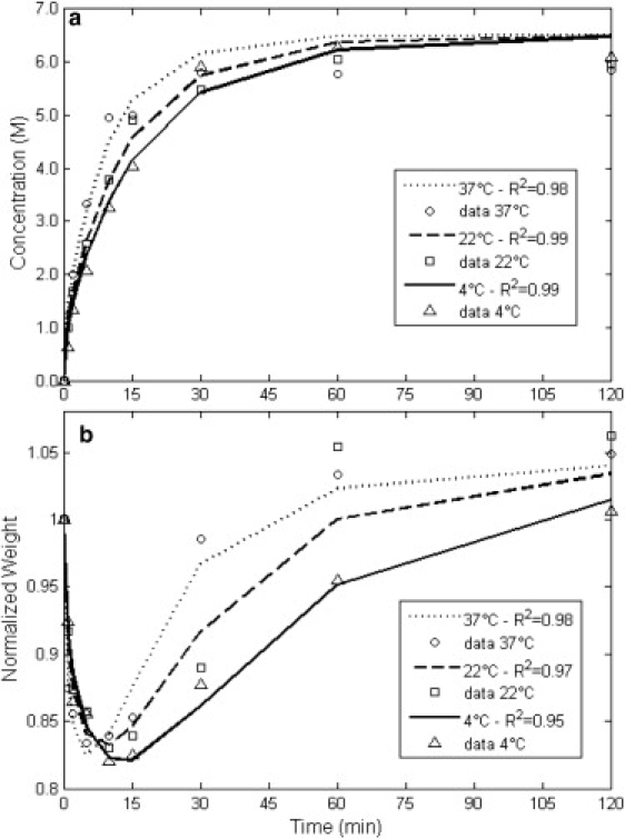
Data of the overall concentration uptake and weight change behavior in disks of cartilage in 6.5 M DMSO solution at 4°C (▵), 22°C (□), and 37°C (○), and the best-fit results for each temperature, 4°C (—), 22°C (---), and 37°C (…).
Figure 6.
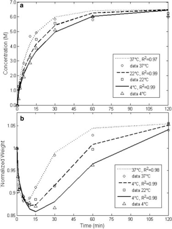
Data of the overall concentration uptake and weight change behavior in disks of cartilage in 6.5 M EG solution at 4°C (▵), 22°C (□), and 37°C (○), and the best-fit results for each temperature, 4°C (—), 22°C (---), and 37°C (…).
It should be noted that, in the experiments, disks of cartilage were exposed to the solution from both sides as well as the circumference. The circumferential surface is smaller than the top and bottom surfaces. In addition, it is reported that the radial permeability of water in cartilage can be 2–10 times less than the axial permeability when the tissue is under static axial compression (18). Therefore, we assume that transport in the radial dimension in the experiments can be ignored and the modeling is done in the axial dimension only. The space reference point x = 0 is different for cartilage disks than when the cartilage is on the bone. Assuming a uniform distribution of the cartilage properties across the thickness of the disks, the space reference is set at the middle of the cartilage, to simulate the conditions of these experiments, so that the top and bottom surfaces of the disk are at x = h(t) and x = −h(t), respectively, where h is half the thickness of the cartilage disk and symmetry holds on both sides of x = 0. The same boundary conditions at x = 0 and x = h(t) still hold, as previously discussed.
Initial and boundary conditions
Equations 25 and 26 were solved with the initial and boundary conditions consistent with the experimental conditions (10). The results were for initial anion concentration M, initial internal pressure P0 = 0.14 MPa, CPA and anion boundary concentrations M and M. The initial solid volume fraction was taken to be 0.2 and the fixed charge density was taken to be an average of 0.2 mEq per gram of tissue water uniformly distributed across the tissue (Table 1). The value of the fixed charge density was taken to be an average of the reported values in the literature, which are between 0.1 and 0.3 mEq per gram of tissue water and an average of 0.2 mEq per gram of tissue water (= 0.2 M)—a physiologically realistic value that is generally accepted and used in the biomechanical engineering literature for cartilage modeling (19). Although there might be species-dependent variability between human and porcine tissue, this range covers the experimentally measured fixed charge density for some species (other than human), such as porcine cartilage (20), which is the experimental model in this study. In this model, there is also a distribution of fixed charge density from the surface to the bone, which is estimated by the average value throughout the cartilage.
It must be mentioned that solving the boundary conditions also results in a positive strain, i.e., swelling, at the boundary of the tissue. As the tensile modulus of cartilage is between one and two orders-of-magnitude higher than its compressive modulus (21), the value of the swelling strain and its effect on the boundary solid volume fraction is very small (∼1%).
Fitting procedure
Equations 1, 5, 7–12, 17, and 20–24 were solved with the COMSOL Multiphysics commercial finite element solver (COMSOL Group, Stockholm, Sweden). Simulations were carried out for the one-dimensional problem as in a slab with half the average thickness of the disks, i.e., 1 mm. The boundary and initial conditions were set as per discussed above. Using a custom-written code in MATLAB (The MathWorks, Natick, MA), values of the four parameters Ksw, Kcs, Dcw, and HA were changed in four nested loops within the ranges introduced in Table 1 and the model was solved for the average CPA concentration and normalized fluid weight as a function of time. A combination of the four parameters returning the least sum of squared errors for both concentration and weight, was taken as the best fit. For Kcs, no values were available; therefore, a wide range of values was considered first and then it was narrowed-down to decrease the time of calculation. If, for any of the parameters, the best-fit value fell on either edge of the initially specified range, then the range for that parameter was extended and the calculation was repeated again in the new extended range.
Results
A numerical analysis was done on the sensitivity of the average CPA concentration and weight change of cartilage disks to the change of each of the four parameters, and the results are presented later in Figs. 1–4. Since the changes in concentration and weight are more significant in the first 30 min, the simulation results are only depicted up to 3 h.
Figure 1.
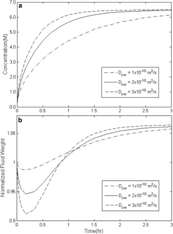
Simulation results of the overall concentration uptake and weight change in disks of cartilage with variable diffusion coefficient Dcw with HA = 3 MPa, Ksw = 5 × 10⁻¹⁶ m4/(N s), and Kcs = 0.2 × 10⁻¹⁶ m4/(N s).
Figure 2.
Simulation results of the overall concentration uptake and weight change in disks of cartilage with variable water permeability Ksw with HA = 1 MPa, Dcw = 3 × 10⁻¹⁰ m2/s, and Kcs = 0.4 × 10⁻¹⁶ m4/(N s).
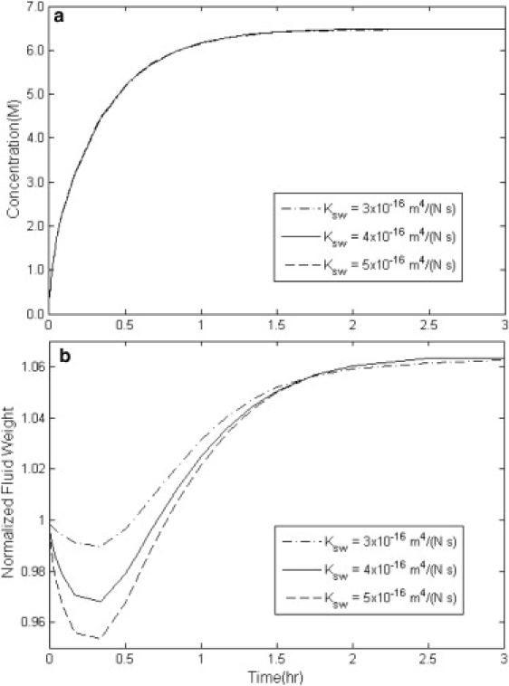
Figure 3.
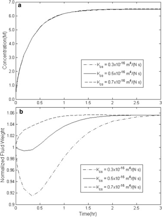
Simulation results of the overall concentration uptake and weight change in disks of cartilage with variable solute permeability Kcs with HA = 1 MPa, Dcw = 3 × 10⁻¹⁰ m2/s, and Ksw = 4 × 10⁻¹⁶ m4/(N s).
Figure 4.
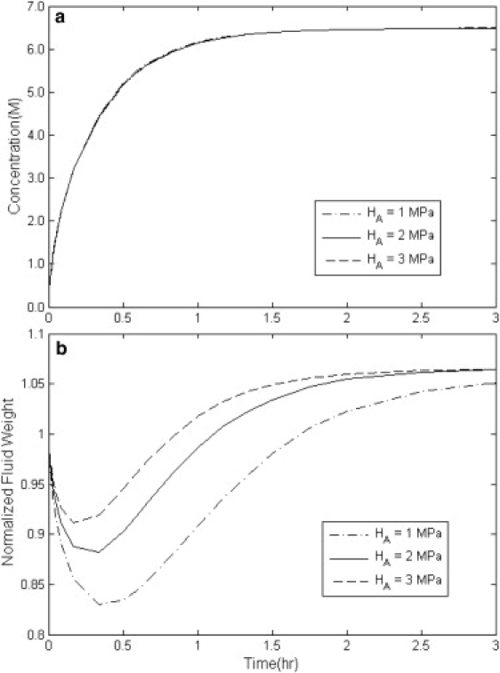
Simulation results of the overall concentration uptake and weight change in disks of cartilage with variable stiffness modulus HA with Dcw = 3 × 10⁻¹⁰ m2/s, Ksw = 5 × 10⁻¹⁶ m4/(N s), and Kcs = 0.2 × 10⁻¹⁶ m4/(N s).
In Fig. 1, a and b, the simulated results of average concentration and weight change behavior of a cartilage disk are plotted for different values of the diffusion coefficient, Dcw. The higher the value of Dcw, the faster the increase in the concentration. The weight change behavior with increasing diffusion coefficient in Fig. 1 b is more complex. The higher the Dcw, the faster the rate of regaining weight. In addition, the minimum weight of the tissue occurs faster and at a lower amount with increasing diffusion coefficient. This can be explained by the fact that with higher Dcw, the concentration of the CPA increases very quickly at the surface layers of the tissue. This introduces a greater chemical potential gradient to the deeper layers of the tissue and causes a greater dehydration so that the minimum weight happens more quickly and at a lower amount.
Fig. 2, a and b, demonstrates the effect of water permeability in cartilage, Ksw, on the concentration increase and weight change of the cartilage. Apparently, Ksw has very little effect on the concentration increase in the tissue. This is also observed in Figs. 3 a and 4 a for CPA permeability, Kcs, and tissue stiffness modulus, HA. In Fig. 2 b, decreasing the value of Ksw from 5 × 10⁻¹⁶ m4/(N s) to 3 × 10⁻¹⁶ m4/(N s) decreases the rate of initial weight loss. Lower Ksw means that the permeation rate of water out of the cartilage gets slower and therefore the tissue loses less water before it reaches equilibrium with the bathing solution.
Fig. 3, a and b, displays how the average concentration and weight of the disk of cartilage change as functions of time with different values of Kcs. By increasing the value of Kcs from 0.3 × 10⁻¹⁶ m4/(N s) to 0.7 × 10⁻¹⁶ m4/(N s), the loss-gain behavior transforms into gain-loss behavior. This suggests that above a certain ratio of Kcs/Ksw, the CPA permeates into the cartilage matrix more quickly than the water leaves it. This either can keep water from leaving the tissue or can cause the water to rush back into the tissue—hence causing an increase in weight before the tissue reaches equilibrium with the surrounding solution.
In Fig. 4, a and b, the effect of different values of the stiffness modulus HA on the average concentration and weight change of cartilage is studied. In Fig. 4 b, with decreasing HA, the minimum weight happens later in time and at lower amounts. To understand this, an analogy with a spring is useful. Under constant compression, the spring with a smaller spring constant—i.e., smaller HA—has the maximum contraction, and vice versa.
In summary, from the results of the numerical analysis, it is understood that each of the four parameters discussed above influences, uniquely, the predictions of the average concentration and weight change, and thus, it is possible to fit the model (uniquely) to the data of average concentration and weight change in cartilage to find (unique) best values of each parameter.
Best-fitted values of the model parameters
Using the fitting procedure described in Materials and Methods, model predictions of average concentration and weight change using the best-fit values of the parameters are plotted in Figs. 5 and 6 for DMSO and EG. Originally, the data was collected up to 24 h. Since the data reaches a plateau after ∼2 h at all three temperatures 4, 22, and 37°C, only the first 2 h are shown in Figs. 5 and 6 and the R2 calculated for each fit is shown on each figure. The best-fit values of each parameter are plotted separately in Figs. 7–10 at three temperatures for DMSO and EG. As another measure of fit sensitivity to the changes in the value of each transport parameter, a range was specified in Figs. 7–10 in which the sum of the squared errors between data and model predictions is less than double the minimum sum of squared errors. This analysis demonstrates how far the value of a parameter can deviate from its best-fitted value before the minimum sum of squared errors doubles. These ranges are depicted in Figs. 7–10 with lines to guide the eyes. This custom analysis can help in understanding, relatively, how well known the values of the fitted parameters are.
Figure 7.
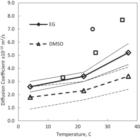
Best-fit results for the diffusion coefficient of DMSO and EG in water in cartilage. Experimental data are measurements of the diffusion coefficients in free solution, DMSO (□) (26) and EG (○) (27). Thin lines denote the ranges of the custom sensitivity analysis.
Figure 8.
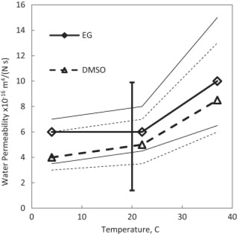
Best-fit results for the water permeability coefficient in cartilage at different temperatures. Thin lines denote the ranges of the custom sensitivity analysis. The solid vertical line shows the range of measurement by others (21) for confined and unconfined compression of cartilage.
Figure 9.
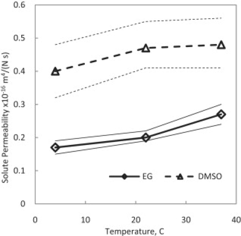
Best-fit results for DMSO and EG permeability coefficient in cartilage at different temperatures. Thin lines denote the ranges of the custom sensitivity analysis.
Figure 10.
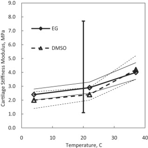
Best-fit results for the stiffness modulus of cartilage at different temperatures. The solid vertical line shows the range of measurements by others (22). Thin lines denote the ranges of the custom sensitivity analysis.
Discussion
Detailed experiments and studies have shown that the compressive aggregate modulus of cartilage, HA, is related to the concentration of the fixed charges and ions as well as solid content in different layers of the cartilage. Because there is a distribution of fixed charges and solid content throughout the thickness of cartilage, the aggregate modulus varies with depth (13). Chen et al. (22) report an increase in the fixed charges density from 0.13 mEq at the surface to 0.25 mEq per gram of tissue water at the bone side in human articular cartilage. The aggregate modulus in the same tissue is reported to increase from 2 MPa to 8 MPa in the respective regions in their study. As mentioned by Chen et al. (22), it is difficult to incorporate these depth-dependent variations into the biomechanical behavior when dealing with transient nonequilibrium conditions. It is even more difficult to do so when the effects of the presence of a solute other than ions in the solution must be incorporated in the model. In addition, our collected data of concentration and weight change are overall measurements. Therefore, to keep the problem tractable, an average was assigned to all properties. Nonetheless, as seen in Figs. 5 and 6, the model is able to describe the weight change at different temperatures uniquely for two different CPAs, with R2 values >0.95.
In Figs. 7–10, it appears that all the four transport parameters considered in this study exhibit some degree of temperature dependence. In Fig. 7, the diffusion coefficients of both EG and DMSO increase with increasing temperature as expected. It is possible to fit this data to an Arrhenius equation to predict, further, the diffusion coefficients at other temperatures. The best-fitted values for the diffusion coefficients of EG and DMSO in water inside cartilage are different from the experimental results for free diffusion of EG and DMSO in water plotted in Fig. 7. It can be hypothesized that the diffusion of EG and DMSO in water is hindered because of the tortuosity of the tissue and the existence of protein molecules in the solution. Nimer et al. (23) measured the diffusion of small noncharged solutes in cartilage and found out that the value of the diffusion coefficient in cartilage reduces to 40% of that in the free solution. Hence, fitted values for Dcw for EG and DMSO plotted in Fig. 7 appear to be consistent with the measurement of Nimer et al. (23).
In Fig. 8, best-fit values of Ksw are plotted for both EG and DMSO at the three temperatures. The indicated areas of our custom sensitivity test are larger compared to those of the other parameters, suggesting that fitting the model to this type of data might not be as accurate for calculation of Ksw. This can be particularly true, as it is shown in the numerical analysis that the major effect of Ksw is on the rate of water loss and therefore the accuracy of the data in first few minutes are very important for the precision of the fit. However, the range of the reported values of Ksw in the literature, between 1.2 × 10⁻¹⁶ m4/(N s) and 10 × 10−16 m4/(N s) (21), still includes the calculated values.
Fig. 9 depicts the temperature dependence of the permeability of the DMSO and EG in cartilage. For both CPAs, the relationship between Kcs and temperature is direct but not very strong. To our knowledge, such a parameter has not been measured or calculated before in any other study, and this article is the first to introduce this parameter and its values calculated indirectly from experiments. It is interesting to note that the permeability values for CPAs are approximately one-order-of-magnitude less than that of water in cartilage.
The best-fit values of cartilage stiffness modulus HA are plotted in Fig. 10. Most mechanical experimentations on cartilage reported in the biomechanical engineering literature have been done on human articular cartilage and, in general, there is no indication of the temperature at which these experiments were conducted. Assuming room temperature, 20°C, as the condition of collecting the data in these experiments, the range of the values for HA for human AC calculated or used in the literature is also plotted in Fig. 10 to compare to the fits for porcine AC. The reported range of HA by Chen et al. (22) for human articular cartilage is 1.2 MPa at the surface layers increasing to 7.5 MPa in deep layers. Theoretically, HA is independent of the type of the CPA used in the experiments. In Fig. 10, values of HA are apparently very close at each temperature regardless of the type of the CPA and are within the reported range of HA in the literature. The apparent temperature dependence for HA might be explained by material properties of collagen as a function of temperature and dependence of the aggregate modulus on the ion concentration, which is a function of temperature.
Conclusion
Based on the triphasic biomechanical description of cartilage, a model has been developed to predict the transient concentration pattern of CPA and water in biological tissues such as cartilage, as well as transient patterns of matrix stress and strain. Values of the parameters regulating the transport of water and solutes in the tissue can be calculated by fitting the model to the data obtained from a simple experimental setup. Fit parameters Ksw and HA appear to be independent of the CPA type, as theoretically expected, and to agree with independent mechanical measurements. Dcw values for both CPAs in cartilage are lower than those in the free solution, again, as expected, and the value of Dcw for DMSO is higher than that of EG, which agrees with the literature for free diffusion. Because the viability of chondrocytes depends highly on the process of loading and unloading the CPA in a cryopreservation protocol, this transient triphasic model for the diffusion of concentrated solutes in cartilage can help researchers understand the fundamental physics of the diffusion problem and can open new doors for tackling the issue of cryopreservation of articular cartilage.
Acknowledgments
This research was funded by the Natural Sciences and Engineering Research Council of Canada and the Canadian Institutes of Health Research (MOP Nos. 85068 and 86492, and CPG No. 75237). Janet A. W. Elliott holds a Canada Research Chair in Interfacial Thermodynamics.
Footnotes
This is an Open Access article distributed under the terms of the Creative Commons-Attribution Noncommercial License (http://creativecommons.org/licenses/by-nc/2.0/), which permits unrestricted noncommercial use, distribution, and reproduction in any medium, provided the original work is properly cited.
References
- 1.Farrant J. Mechanism of cell damage during freezing and thawing and its prevention. Nature. 1965;205:1284–1287. [Google Scholar]
- 2.Fahy G.M., MacFarlane D.R., Angell C.A., Meryman H.T. Vitrification as an approach to cryopreservation. Cryobiology. 1984;21:407–426. doi: 10.1016/0011-2240(84)90079-8. [DOI] [PubMed] [Google Scholar]
- 3.Pegg D.E. The current status of tissue cryopreservation. Cryo Letters. 2001;22:105–114. [PubMed] [Google Scholar]
- 4.Muldrew K., Sykes B., Schchar N., McGann L.E. Permeation kinetics of dimethyl sulfoxide in articular cartilage. Cryo Letters. 1996;17:331–340. [Google Scholar]
- 5.Jomha N.M., Lavoie G., Muldrew K., Schachar N.S., McGann L.E. Cryopreservation of intact human articular cartilage. J. Orthop. Res. 2002;20:1253–1255. doi: 10.1016/S0736-0266(02)00061-X. [DOI] [PubMed] [Google Scholar]
- 6.Pegg D.E., Wusteman M.C., Wang L. Cryopreservation of articular cartilage. 1: Conventional cryopreservation methods. Cryobiology. 2006;52:335–346. doi: 10.1016/j.cryobiol.2006.01.005. [DOI] [PubMed] [Google Scholar]
- 7.Muldrew K., Novak K., Studholme C., Wohl G., Zernicke R. Transplantation of articular cartilage following a step-cooling cryopreservation protocol. Cryobiology. 2001;43:260–267. doi: 10.1006/cryo.2001.2349. [DOI] [PubMed] [Google Scholar]
- 8.Elmoazzen H.Y., Poovadan A., Law G.K., Elliott J.A.W., McGann L.E. Dimethyl sulfoxide toxicity kinetics in intact articular cartilage. Cell Tissue Bank. 2007;8:125–133. doi: 10.1007/s10561-006-9023-y. [DOI] [PubMed] [Google Scholar]
- 9.Pegg D.E., Wang L., Vaughan D. Cryopreservation of articular cartilage. 3: The liquidus-tracking method. Cryobiology. 2006;52:360–368. doi: 10.1016/j.cryobiol.2006.01.004. [DOI] [PubMed] [Google Scholar]
- 10.Jomha N.M., Law G.K., Abazari A., Rekieh K., Elliott J.A.W. Permeation of several cryoprotectant agents into porcine articular cartilage. Cryobiology. 2009;58:110–114. doi: 10.1016/j.cryobiol.2008.11.004. [DOI] [PubMed] [Google Scholar]
- 11.Sharma R., Law G.K., Rekieh K., Abazari A., Elliott J.A.W. A novel method to measure cryoprotectant permeation into intact articular cartilage. Cryobiology. 2007;54:196–203. doi: 10.1016/j.cryobiol.2007.01.006. [DOI] [PubMed] [Google Scholar]
- 12.Mow V.C., Kuei S.C., Lai W.M., Armstrong C.G. Biphasic creep and stress relaxation of articular cartilage in compression: theory and experiments. J. Biomech. Eng. 1980;102:73–84. doi: 10.1115/1.3138202. [DOI] [PubMed] [Google Scholar]
- 13.Lai W.M., Hou J.S., Mow V.C. A triphasic theory for the swelling and deformation behavior of articular cartilage. J. Biomech. Eng. 1991;113:245–258. doi: 10.1115/1.2894880. [DOI] [PubMed] [Google Scholar]
- 14.Gu W.Y., Lai W.M., Mow V.C. Transport of fluid and ions through a porous-permeable charged-hydrated tissue and streaming potential data on normal bovine articular cartilage. J. Biomech. 1993;26:709–723. doi: 10.1016/0021-9290(93)90034-c. [DOI] [PubMed] [Google Scholar]
- 15.Shaozhi Z., Pegg D.E. Analysis of permeation of cryoprotectant in cartilage. Cryobiology. 2007;54:146–153. doi: 10.1016/j.cryobiol.2006.12.001. [DOI] [PubMed] [Google Scholar]
- 16.Elliott J.A.W., Prickett R.C., Elmoazzen H.Y., Porter K.R., McGann L.E. A multisolute osmotic virial equation for solutions of interest in biology. J. Phys. Chem. 2007;111:1775–1785. doi: 10.1021/jp0680342. [DOI] [PubMed] [Google Scholar]
- 17.Elmoazzen H.Y., Elliott J.A.W., McGann L.E. Osmotic transport across cell membranes in nondilute solutions: a new nondilute solute transport equation. Biophys. J. 2009;96:2559–2571. doi: 10.1016/j.bpj.2008.12.3929. [DOI] [PMC free article] [PubMed] [Google Scholar]
- 18.Reynaud B., Quinn T.M. Anisotropic hydraulic permeability in compressed articular cartilage. J. Biomech. 2006;39:131–137. doi: 10.1016/j.jbiomech.2004.10.015. [DOI] [PubMed] [Google Scholar]
- 19.Mow V.C., Ateshian G.A., Lai W.M., Gu W.Y. Effects of fixed charges of the stress relaxation behavior of hydrated soft tissues in confined compression problem. Int. J. Solids Struct. 1998;35:4945–4962. [Google Scholar]
- 20.Lu X.L., Miller C., Chen F.H., Guo X.E., Mow V.C. The generalized triphasic correspondence principle for simultaneous determination of the mechanical properties and proteoglycan content of articular cartilage by indentation. J. Biomech. 2007;40:2434–2441. doi: 10.1016/j.jbiomech.2006.11.015. [DOI] [PubMed] [Google Scholar]
- 21.Mow V.C., Guo X.E. Mechano-electrochemical properties of articular cartilage: their inhomogeneities and anisotropies. Annu. Rev. Biomed. Eng. 2002;4:175–209. doi: 10.1146/annurev.bioeng.4.110701.120309. [DOI] [PubMed] [Google Scholar]
- 22.Chen S.S., Falcovitz Y.H., Schneiderman R., Maroudas A., Sah R.L. Depth-dependent compressive properties of normal aged human femoral head articular cartilage: relationship to fixed charge density. Osteoarthritis Cartilage. 2001;9:561–569. doi: 10.1053/joca.2001.0424. [DOI] [PubMed] [Google Scholar]
- 23.Nimer E., Schneiderman R., Maroudas A. Diffusion and partition of solutes in cartilage under static load. Biophys. Chem. 2003;106:125–146. doi: 10.1016/s0301-4622(03)00157-1. [DOI] [PubMed] [Google Scholar]
- 24.Prickett R.C., Elliott J.A.W., McGann L.E. Application of the osmotic virial equation in cryobiology. Cryobiology. 2009 doi: 10.1016/j.cryobiol.2009.07.011. Accepted. [DOI] [PubMed] [Google Scholar]
- 25.Chowdhuri S., Chandra A. Tracer diffusion of ionic and hydrophobic solutes in water–dimethyl sulfoxide mixtures: effects of varying composition. J. Chem. Phys. 2003;119:4360–4366. [Google Scholar]
- 26.Holz M., Heil S.R., Sacco A. Temperature-dependent self-diffusion coefficients of water and six selected molecular liquids for calibration in accurate 1H NMR PFG measurements. Phys. Chem. Chem. Phys. 2000;2:4740–4742. [Google Scholar]
- 27.Ternström G., Sjöstrand A., Aly G., Jernqvist Å. Mutual diffusion coefficients of water+ethylene glycol and water+glycerol mixtures. J. Chem. Eng. Data. 1996;41:876–879. [Google Scholar]
- 28.Gu W.Y., Lai W.M., Mow V.C. A mixture theory for charged-hydrated soft tissues containing multi-electrolytes: passive transport and swelling behaviors. J. Biomech. Eng. 1998;120:169–180. doi: 10.1115/1.2798299. [DOI] [PubMed] [Google Scholar]
- 29.Yao H., Gu W.Y. Convection and diffusion in charged hydrated soft tissues: a mixture theory approach. Biomech. Model. Mechanobiol. 2007;6:63–72. doi: 10.1007/s10237-006-0040-3. [DOI] [PMC free article] [PubMed] [Google Scholar]