Elasticity Imaging of Polymeric Media

Abstract

Viscoelastic properties of soft tissues and hydropolymers depend on the strength of molecular bonding forces connecting the polymer matrix and surrounding fluids. The basis for diagnostic imaging is that disease processes alter molecular-scale bonding in ways that vary the measurable stiffness and viscosity of the tissues. This paper reviews linear viscoelastic theory as applied to gelatin hydrogels for the purpose of formulating approaches to molecular-scale interpretation of elasticity imaging in soft biological tissues. Comparing measurements acquired under different geometries, we investigate the limitations of viscoelastic parameters acquired under various imaging conditions. Quasistatic (step-and-hold and low-frequency harmonic) stimuli applied to gels during creep and stress relaxation experiments in confined and unconfined geometries reveal continuous, bimodal distributions of respondance times. Within the linear range of responses, gelatin will behave more like a solid or fluid depending on the stimulus magnitude. Gelatin can be described statistically from a few parameters of low-order rheological models that form the basis of viscoelastic imaging. Unbiased estimates of imaging parameters are obtained only if creep data are acquired for greater than twice the highest retardance time constant and any steady-state viscous response has been eliminated. Elastic strain and retardance time images are found to provide the best combination of contrast and signal strength in gelatin. Retardance times indicate average behavior of fast (1–10 s) fluid flows and slow (50–400 s) matrix restructuring in response to the mechanical stimulus. Insofar as gelatin mimics other polymers, such as soft biological tissues, elasticity imaging can provide unique insights into complex structural and biochemical features of connectives tissues affected by disease.

1 Introduction

There exist several techniques for imaging spatiotemporal distributions of mechanical properties in biological tissues and engineered constructs on scales from molecules to organs. Collectively, they are known as elasticity imaging. Diagnostic techniques employ phase-sensitive imaging modalities capable of tracking local tissue movements induced by a mechanical stimulus. The resulting image displays components of displacement or strain and sometimes a compliance or modulus. For example, ultrasonic and magnetic resonance (MR) techniques are frequently applied to breast tissues to image viscoelastic properties of tumors [1–3]. The principal advantage of elasticity imaging is the large object contrast for tissue stiffness [4] that occurs within stromal tissues in response to the advancing disease [5,6]. Another large application area is vascular elasticity imaging using MR [7], optical [8], x-ray [9], and ultrasonic [10] methods. Emerging applications include viscoelastic imaging of macromolecules [11] and engineered tissue constructs [12]. The excitement about elasticity imaging is extending beyond diagnosis as we increase our understanding of the role of cellular mechanochemical transduction [13], particularly in cancer [5] and atherosclerosis [14].

Clinical elasticity imaging of breast cancer patients shows that malignant tumors most frequently appear as stiff regions (low strain or high modulus) compared to background media [15,16]. Stiffening is common because of edema, cellular hyperplasia, and characteristic increases in stromal collagen concentration and cross-linking. However, cancers can also appear softer than the background tissue [17] because the magnitude, spatial homogeneity, and temporal variation of the strain response depend on the physiology [18] and tumor microenvironment [6] of a specific patient. In addition, images of viscoelastic features show both lower [19] and higher [2,3] respondance times for malignant masses as compared to benign masses. Although electron microscopy data show changes in the connective tissue ultrastructure [20] that suggest lower viscosity, not enough is known about the viscoelastic behavior of breast tissues in vivo to determine if the diversity of findings are due to patient or experimental variabilities. To advance diagnostic applications, we must discover how disease-related changes to molecular bonding within stromal tissues affect the broad spectrum of viscoelastic responses. This is essentially the inverse problem of estimating structural features of polymers from measured mechanical properties.

This paper reviews classical linear theory for polymers undergoing standard mechanical (quasi-static) stimuli in the context of ultrasonic strain imaging. We investigate the role of discrete rheological models (Voigt and Maxwell) that offer concise parametric summaries of viscoelastic behavior. Measurements of gelatin gels with different experimental geometries test the validity of model assumptions, show the consequences of violations, and define ultrasonic imaging parameters required for strain imaging. Gelatin shares a basic structure and many features of stromal breast tissues, and yet it is a simpler medium with adjustable mechanical properties. Therefore, gelatin gels are excellent media for investigating the strengths and weaknesses of elasticity imaging. One long-term goal of elasticity imaging research is to interpret micro-structural reorganization of connective tissues during cancer progression from the macroscopic deformation patterns in viscoelastic images. Our experience with gelatin provides a framework for future tissue investigations.

2 Methods

This section reviews constitutive equations for the experimental geometries used in this study, including strain imaging where stress and strain vary in space and time. Imaging techniques often apply stresses and measure time-varying strain patterns; therefore, the discussion is focused on creep. Results from other geometries and stimuli allow comparisons for validating imaging techniques.

2.1 Constitutive Equation

Assume a small cubic volume of gelatin is centered at vector position x. Applying a weak force to volume surfaces at time t=t₀ produces infinitesimal stresses dσ_ij(x, t′), where t′ = (t − t₀). These induce infinitesimal strains dϵ_ij(x, t)=S_ijkl(x,t − t′)dσ_kl(x,t′) for t ′ > 0, where the material properties of the medium are elements of the fourth-order compliance tensor S_ijkl. In media with linear time-invariant material properties, strains histories can be superimposed [21,22] to find

$${\mathbf{ϵ}}_{\mathit{\text{ij}}}(\mathbf{x},t)={\displaystyle {\int }_0^{t}dt\prime S_{\mathit{\text{ijkl}}}}(\mathbf{x},t-t\prime )\frac{\partial {\sigma }_{\mathit{\text{kl}}}}{\partial t\prime }(\mathbf{x},t\prime )$$ (1)

Equation (1) describes time-varying strain for volume elements within a linear viscoelastic medium, and thus it also describes the strain image of a deformed object.

Adopting the notation $\widetilde{\mathbf{ϵ}}(\mathbf{x},s)=\mathcal{L}\mathbf{ϵ}(\mathbf{x},t)={\displaystyle {\int }_0^{\infty }\mathit{\text{dt}}\text{exp}(-\mathit{\text{st}})\mathbf{ϵ}(\mathbf{x},t)}$ for the one-sided Laplace transform, Eq. (1) becomes

$${\widetilde{\mathbf{ϵ}}}_{\mathit{\text{ij}}}(\mathbf{x},s)=s{\tilde{S}}_{\mathit{\text{ijkl}}}(\mathbf{x},s){\tilde{\sigma }}_{\mathit{\text{kl}}}(\mathbf{x},s)$$ (2)

Here, s is a complex variable fundamental to the Laplace transform. For isotropic media, S can be expanded to give the generalized viscoelastic Hooke’s law (cf. Eq. (11.2–8) [23])

$${\widetilde{\mathbf{ϵ}}}_{\mathit{\text{ij}}}(\mathbf{x},s)=\left(\frac{1}{9}s\tilde{B}(\mathbf{x},s)-\frac{1}{6}s\tilde{J}(\mathbf{x},s)\right)\tilde{\sum }(\mathbf{x},s){\delta }_{\mathit{\text{ij}}}+\frac{1}{2}s\tilde{J}(\mathbf{x},s){\tilde{\sigma }}_{\mathit{\text{ij}}}(\mathbf{x},s)$$ (3)

where Σ̃(x,s) = σ̃₁₁(x,s)+σ̃₂₂(x,s)+σ̃₃₃(x,s) is the trace of the stress matrix and δ_ij is the Kronecker delta. B̃(x,s) is bulk compliance that describes volume changes in the medium and J̃(x,s) is shear compliance that describes shape changes, both in the Laplace domain. The subscripts kl, ij are interchangeable since the stress and strain tensors are the same size and have only six independent terms.

The task now is to formulate stress tensors for different measurement conditions and apply Eq. (3) to predict strain. In this manner, the results of standard measurement techniques with known geometry can be compared to those of imaging experiments where the geometry is less well known.

2.2 Uniaxial Compressive Stress: Creep

Our imaging experiments involve application of a uniaxial compressive stress under free-slip boundary conditions. Ideally, this experiment generates only one nonzero stress element, i.e., σ̃₁₁, and three normal strains, although ϵ˜₂₂=ϵ˜₃₃ for isotropic materials. Solving Eq. (3) for the strain tensor corresponding to the applied stress yields

$${\widetilde{\mathbf{ϵ}}}_{11}(\mathbf{x},s)=\left(\frac{1}{9}s\tilde{B}(\mathbf{x},s)+\frac{1}{3}s\tilde{J}(\mathbf{x},s)\right){\tilde{\sigma }}_{11}(\mathbf{x},s)$$ (4)

For ultrasonic strain imaging, strain is estimated along the axis of the sound beam and in the direction of the applied force x₁. Consequently, ϵ˜₁₁ in Eq. (4) is often referred to as axial strain in imaging experiments [24]. Axial strain images are common because ultrasonic echoes are most sensitive to object movements along the phase-sensitive beam axis. In the following, ϵ˜ indicates ϵ˜₁₁ except where otherwise noted.

From one strain measurement, however, only the linear combination of shear and bulk compliances can be determined. Thus, we study the measurable quantity compressive compliance [23], D̃(x,s)=(1/9) B̃(x,s)+(1/3)J̃(x,s), where

$$\widetilde{\mathbf{ϵ}}(\mathbf{x},s)=s\tilde{D}(\mathbf{x},s){\tilde{\sigma }}_{11}(\mathbf{x},s)$$ (5)

The literature on creep measurements in collagen [25] and gelatin gels [26,27] provides guidance on modeling compliance. A generalized Voigt model is often useful [23,28]

$$s\tilde{D}(\mathbf{x},s)=D_0+{\displaystyle \sum _{\ell =1}^L\frac{D_{\ell }}{1+s{T}_{\ell }}+\frac{1}{s{\eta }_0}}$$ (6)

Constants D_ℓ are compressive creep compliances, and T_ℓ are discrete retardation times that are proportional to viscosity coefficients η_ℓ of the ℓth viscoelastic component: T_ℓ=D_ℓ η_ℓ. If we can eliminate the last term in Eq. (6) and let T_L be the largest time constant, the Fourier transform of compliance will exist because the region of convergence, i.e., s > −1/T_L, includes the imaginary axis. Equation (6) implies a time-independent elastic strain and L distinct viscoelastic strains that delay in time the full response. The last term describes the steady-state compressive-flow viscosity coefficient η₀. In weakly compressed tissues, η₀ may represent flow of vascular fluids; in hydrogels it represents movement of unbound water.

A constant uniaxial force F₁ is suddenly applied at t₀ to a cubic sample of side-area A along the x₁ axis. Then σ₁₁(x,t)=σ_a(x)u(t − t₀), where σ_a=F₁/A for the volume element located at x, and the step function u(t−t₀) is zero for t < t₀ and one for t ≥ t₀. The Laplace transform of the step stress stimulus is

$${\tilde{\sigma }}_{11}(\mathbf{x},s)={\sigma }_a(\mathbf{x})/s$$ (7)

Combining Eq. (5)–Eq. (7) and taking the inverse Laplace transform yields for t > t₀

$$\mathbf{ϵ}(\mathbf{x},t)={\mathbf{ϵ}}_0(\mathbf{x})+{\displaystyle \sum _{\ell =1}^L{\mathbf{ϵ}}_{\ell }(\mathbf{x})\{1-\text{exp}[-(t-t_0)/T_{\ell }(\mathbf{x})]\}+(t-t_0)\frac{{\sigma }_a(\mathbf{x})}{{\eta }_0(\mathbf{x})}}$$ (8)

where strain amplitudes ϵ_ℓ = σ_aD_ℓ for 0 ≤ ℓ ≤ L. The strain response of the Voigt model to a step load in time has three components.

The initial elastic response occurs immediately after compression, i.e., ϵ(x,t₀+) ⋍ ϵ₀(x), before the viscous mechanisms have time to engage. Purely elastic responses are implicitly assumed in “static” elastography techniques that ignore time-varying strain [24,29,30]. If σ_a(x) = σ_a is constant throughout the volume, then the instantaneous elastic response is directly proportional to the compressive compliance D₀ (and inversely proportional to the elastic modulus E₀) in the volume element. Stresses in heterogeneous media, whose volume elements have unknown boundary conditions, vary unpredictably with position. Strain images in such media must be carefully interpreted to infer stiffness.

The second term defines the time-varying viscoelastic (VE) response: ϵ_VE(x,t)=ϵ(x,t)−ϵ₀(x)−(t−t₀)σ_a(x)/η₀(x). In solids, strain builds exponentially over time with rate constants T_ℓ until the total strain reaches the steady-state value ${\sum }_{\ell =0}^L{\mathbf{ϵ}}_{\ell }(\mathbf{x})$ at t ≫ T_L(x). Measurable viscoelastic responses are from breakage and reformation of weak molecular bonds, release of polymer filament entanglements [28], and other internal restructuring.

The third term in Eq. (8), which varies linearly in time, describes viscous flow within the polymer; e.g., curve a in Fig. 1(a). If time-varying strain plateaus (curve b), the polymer behaves as a solid. VE solids are modeled with Eq. (8) by setting the last term to zero. Model parameters D_ℓ, T_ℓ, and η₀ that vary spatially are candidate parameters for diagnostic imaging. Because σ_a(x) is unknown in practice, we study ϵ_ℓ=D_ℓσ_a in place of D_ℓ.

Fig. 1.

(a) Creep curves for a second-order (L=2) Voigt model and a step stress stimulus are illustrated. Curve a is drawn directly from Eq. (8) with finite η₀; its slope at t ≫ T₂ is σ_a/η₀. Curve b is from the same equation where η₀=∞. In both cases, ϵ₂/ϵ₁ = 2.5, T₁=3 s, and T₂=100 s. (b) The corresponding Fourier spectra D̆(ω) are from Eq. (10). Spectra from a step and 1 s ramp stress stimulus are compared.

Ultimately, the value of ϵ_ℓ, T_ℓ, and η₀ as diagnostic imaging features depends on their sensitivity and specificity to disease-related changes in tissue structure and biochemistry [6]. The discrete compliance model of Eq. (6) is attractive because it offers a testable number of parameters that may be interpreted in terms of polymer structure. Fung [21] and others warn against determining the order of the model by blindly fitting model functions to data. The retardation spectrum [28,31] described below provides another tool for estimating retardance time distributions.

First, we examine the Fourier spectrum of the VE creep response in two ways. One describes the spectrum of the creep measurement ϵ˜_VE(ω) to determine sampling requirements. Strain is sampled in time at the frame rate of the ultrasound system. Another describes the frequency spectrum of the medium response D˘(ω).

Fourier Spectra

The Fourier transform of the VE response to a uniaxial step stress may be found from the Laplace domain representation of Eq. (5)–Eq. (7) by substituting s = iω

$${\widetilde{\mathbf{ϵ}}}_{\text{VE}}(\omega )=\frac{1}{i\omega }{\displaystyle \sum _{\ell =1}^L{\mathbf{ϵ}}_{\ell }\left(\frac{1-i\omega T_{\ell }}{1+{\omega }^2{T}_{\ell }^2}\right)}$$ (9)

ω is angular temporal frequency in rad/s and $i=\sqrt{-1}$. If T₁ is the smallest time constant, then the ℓ = 1 term determines the highest frequency in the response bandwidth. The frequency spectrum of this creep component is $|{\widetilde{\mathbf{ϵ}}}_{\text{VE}}(\omega )|={\mathbf{ϵ}}_1/(\omega \sqrt{1+{\omega }^2{T}_1^2})\to {\mathbf{ϵ}}_1/{\omega }^2{T}_1$ for ω ≫ 1/T₁. The measurement spectrum decreases monotonically as ω⁻² and thus is bandlimited.

Of great interest is the frequency spectrum of material properties; specifically, the loss spectrum for compressive compliance D˘(ω) [23]. From Eq. (5) and Eq. (6)

$${\breve{D}(\omega )\triangleq \omega \tilde{D}(\omega )=-\text{Im}\frac{s{\widetilde{\mathbf{ϵ}}}_{\text{VE}}(s)}{{\sigma }_a}|}_{s=i\omega }={\displaystyle \sum _{\ell =1}^L\frac{D_{\ell }\omega T_{\ell }}{1+{\omega }^2{T}_{\ell }^2}}$$ (10)

where Im is the imaginary part of what follows. The procedure for estimating D˘(ω) from creep data begins by eliminating the elastic and steady-state viscous terms to find ϵ_VE(t). We then multiply by a Shepp-Logan-type high-pass filter [32] and next compute the Fourier transform, which yields a stable estimate of sϵ˜_VE(s)_s=iω in the presence of noise. The loss compliance spectrum for a second-order Voigt model is displayed on a semi-log plot in Fig. 1(b). Curve parameters are given in the caption.

Figure 1(b) shows the Nyquist frequency to be f_N=ω_N/2π ⋍ 1.5 Hz, requiring a frame rate of at least 3 Hz to faithfully record creep with T_ℓ≥3 s. To visualize the lowest frequency peak at ω₂ in this example, corresponding to T₂=100 s, the acquisition time should be (2π)/ω₂>628 s, preferably longer. Acquiring data for shorter times truncates the spectrum at low frequencies without distorting higher frequency values, but creates difficulties in determining model order from data as described below. In vivo breast imaging techniques allow patient acquisition times between 20 and 200 s. Acquisitions in hydrogel samples are often on the order of 2500 s.

The two peaks in the frequency spectrum arise from L=2 roots (nonzero poles of Eq. (6)) at s=−1/T_ℓ; both are real and negative. They correspond to spectral peaks at ω_ℓ=1/T_ℓ [33], of height D_ℓ/2, and −6 dB peak width $∆{\omega }_{\ell }=2\sqrt{3}/T_{\ell }$. The latter property shows that T_ℓ must be widely separated to resolve their peaks on the frequency axis. The pole at s = 0 from the steady-state viscosity term must be eliminated for the Fourier transform to exist. Poles of the model uniquely determine the time-varying properties of the material.

Retardation Spectra

It is attractive to adopt a discrete model for compliance; e.g., Eq. (6). Low-order models with few components that correspond to specific structural and biochemical features yield the diagnostic imaging parameters we seek. However, data from tissues [21] and gels [28] suggest broad continuous distributions of retardance times τ. Schwarzl and Staverman [31] proposed a technique for estimating continuous spectra L(τ) from creep data. To facilitate direct comparisons with Fourier spectra, we plot L̃(ω)=L(τ)|_ω=1/τ. The two forms of L are refections of each other about the ordinate, followed by a translation along the logarithmic abscissa.

L(τ) is introduced by considering the Laplace transform of Eq. (8) for a step stress stimulus and a continuous distribution of compliance

$$\tilde{D}(\mathbf{x},s)=\frac{D_0(\mathbf{x})}{s}+{\displaystyle {\int }_0^{\infty }d\tau \frac{D_s(\mathbf{x},\tau )}{s(1+s\tau )}+\frac{1}{s^2{\eta }_0(\mathbf{x})}}$$ (11)

where D_s(x, τ) is the sampled compliance function obtained when the discrete sum is converted into an integral as shown in [34]. Substituting L(τ) = τD_s(τ) and noting that d ln τ=dτ/τ and τ=τ(x), the inverse Laplace transform of Eq. (11) for t>t₀ is

$$D(\mathbf{x},t)=D_0(\mathbf{x})+{\displaystyle {\int }_{-\infty }^{\infty }d\text{ln}\tau L(\mathbf{x},\tau )\{1-\text{exp}[-(t-t_0)/\tau ]\}+\frac{(t-t_0)}{{\eta }_0(\mathbf{x})}}$$ (12)

A method for estimating L from creep compliance estimates D^_VE was described by Tschoegl [23]:

$${L(\mathbf{x},\tau )=\underset{k\to \infty }{\text{lim}}\frac{{(-1)}^{k-1}}{(k-1)!}{\mathcal{D}}_t^{(k)}{\widehat{D}}_{\text{VE}}(\mathbf{x},t)|}_{t=k\tau }$$ (13)

${\mathcal{D}}_t^{(k)}={\mathcal{D}}_t({\mathcal{D}}_t-1)({\mathcal{D}}_t-2)\cdots ({\mathcal{D}}_t-k+1)$ is a factorial-like derivative and 𝒟_t=d/d ln t is the derivative operator. The first- and second-order approximations are

$$\begin{array}{c}{L^{(1)}(\mathbf{x},\tau )=\frac{d}{d\text{ln}t}{\widehat{D}}_{\text{VE}}(\mathbf{x},t)|}_{t=\tau }\\ L^{(2)}(\mathbf{x},\tau )={\left[\frac{d}{d\text{ln}t}{\widehat{D}}_{\text{VE}}(\mathbf{x},t)-\frac{d^2}{d{(\text{ln}t)}^2}{\widehat{D}}_{\text{VE}}(\mathbf{x},t)\right]}_{t=2\tau }\end{array}$$ (14)

The kth-order estimate L^(k)(τ) is found by first filtering creep data with a low-pass polynomial filter using matlab® 7. Specifically, P(:,j)=polyfit(log(t), y, N(j)), where P is a (N + 1) × 12 matrix of polynomial coefficients and y ≜ D^_VE(x, n∆t) time samples. As the polynomial order is increased from 4≤N(j) ≤ 15, the frequency response of the jth filter is plotted from the magnitude of the function freqz(P(:,j),Z), where Z is a vector of ones. The lowest-order filter spectrum maximally flat in the stop band and with a smooth transition region is selected by visual inspection to represent the data. Filter order depends on the bandwidth of the VE response: short-duration time constants require higher-order polynomial filters. The derivatives of Eq. (13) are computed analytically from the polynomial representation.

To develop stopping rules for selecting k in Eq. (13), we generated noiseless creep data assuming a log-normal input distribution of retardance times [23]. The input function L̃(ω) is represented by the open circles in Fig. 2. Clearly, it is difficult to describe the input distribution of τ from its Fourier spectrum D˘(ω) of Fig. 2(a) even though the ratio of peak frequencies is 30. Conversely, retardation spectral estimates approach the input distribution as k increases. Narrow distributions require large k values to minimize bias. However, estimates become unstable as k increases, placing greater emphasis on filter design.

Fig. 2.

(a) Retardation spectra from simulated data. Plotted are L̃(ω)=L(τ)|_τ=1/ω for comparison with the Fourier spectrum. Creep data were generated from Eq. (12) for ϵ₀=σ_a/η₀ = 0 assuming a broadband, bimodal input as given by the circle points (Input). Estimated retardation spectra (RS) L^(k)(ω) for k=1,2,5,6, are compared to the Fourier spectrum (FS) D̆(ω), computed from the same data. (b) L̃⁽⁶⁾ estimates without noise in the creep data and with noise (signal-to-noise ratio=32.2 dB). A ninth-order polynomial filter was applied to the noisy data before estimation.

The effects of measurement noise are shown in Fig. 2(b). Adding white Gaussian noise with signal-to-noise ratio 32.2 dB (typical of rheometer data described below) introduces bias particularly at high frequency. Figure 3 predicts the amount of bias introduced as the width of the log-normal input distribution increases. The data suggest that a 150 s bandwidth can be estimated with acceptable bias by a sixth-order estimate L⁽⁶⁾(τ).

Fig. 3.

Limitation of L^(k)(τ) for representing retardance time distributions. The abscissa is b/a from the log-normal input distribution L(τ)=exp[−(ln τ−a)²/2b²]. The ordinate is the full-width-at-half-maximum bandwidth of retardance spectral estimates. Circles denote the exact output bandwidth for the input distribution, while the curves are bandwidths for kth-order estimates using noiseless creep data. Results suggest that the L⁽⁶⁾(τ) represents bandwidths of log-normal distributions above 150 s with acceptable bias error.

2.3 Shear Stress and Strain

The unconfined boundaries of arbitrarily shaped, heterogeneous media subjected to uniaxial stress stimuli in imaging experiments can violate the assumptions leading to Eq. (3). To study the effects, we compare parameters from the carefully controlled geometry of standard rheometer measurements to those from creep imaging experiments. Our interest is with average properties, so the positional dependence is ignored for these nonimaging measurements.

The constitutive equation is calculated in the Laplace domain from Eq. (3)

$${\widetilde{\mathbf{ϵ}}}_{12}(s)=\frac{1}{2}s\tilde{J}(s){\tilde{\sigma }}_{12}(s)$$ (15)

Bulk compliance terms are negligible in rotational shear measurements. For a step shear stress, ${\sigma }_{12}={\sigma }_a^{\prime }u(t-t_0)$, and assuming the Voigt model in shear, the observed creep in the time domain is

$$\begin{array}{ll}{\gamma }_{12}(t)=\hfill & {\gamma }_{(12)0}+{\displaystyle \sum _{m=1}^M{\gamma }_{(12)m}\{1-\text{exp}[-(t-t_0)/T_m]\}}\hfill \\ \hfill & +(t-t_0)\frac{{\sigma }_a^{\prime }}{{\eta }_0^{\prime }}\text{\hspace{1em}for}t>t_0\hfill \end{array}$$ (16)

Measurable shear creep is related to the corresponding strain tensor via γ₁₂=2ϵ₁₂ [23]. In addition, ${\gamma }_{(12)m}={\sigma }_a^{\prime }{J}_m$ for 0 ≤ m ≤ M and ${\eta }_0^{\prime }$ is the steady-state shear-flow viscosity coefficient. To account for the geometry of the cone-plate viscometer, the ratio γ₁₂(t)/σ₁₂(t) = λ φ/Γ, where φ is the angular displacement, Γ is the applied torque, and λ = 2πR³/3ϕ is a geometric factor that depends on the radius of the cone (R=30 mm) and on the angle between the cone and plate (ϕ=4 deg).

Compression and shear measurements may be compared through Eq. (8) and Eq. (16). Compressive and shear creep compliances are, respectively

$$\begin{array}{l}D(t)={\mathbf{ϵ}}_{11}/{\sigma }_a=D_0+{\displaystyle \sum _{\ell }}{D}_{\ell }[1-\text{exp}(-t\prime /T_{\ell })]+t\prime /{\eta }_0\hfill \\ J(t)={\gamma }_{12}/{\sigma }_a^{\prime }=J_0+{\displaystyle \sum _m}{J}_m[1-\text{exp}(-t\prime /T_m)]+t\prime /{\eta }_0^{\prime }\hfill \end{array}$$ (17)

for t′ = t − t₀>0. From Eq. (4) and Eq. (5) we have D(t)=J(t)/3+B(t)/9. Thus, model parameters for the two experiments may be compared directly only for “incompressible media” where bulk compliance B(t) is negligible. Bulk compliance can be related to compressive compliance and Poisson’s ratio in the Laplace domain: sB̃(s)=3sD̃(s)[1−2sν̃(s)], where sν̃(s) =−ϵ˜₂₂(s)/ϵ˜₁₁(s). We can then use limit theorems [23] to find in the time domain B(∞) = 3D(∞)(1−2ν(∞)) at s → 0 and B(0) = 3D(0)(1−2ν(0)) at s → ∞.

2.4 Uniaxial Compressive Strain: Stress Relaxation and Relaxation Spectra

Stress relaxation experiments are conducted in which samples are stimulated with a uniaxial step strain while stress is measured over time. This nonimaging technique provides spectral data under confined boundary conditions that could not be obtained using creep measurements with our instruments.

Analogous to Eq. (3), the generalized viscoelastic Hooke’s law for stress relaxation is [23]

$${\tilde{\sigma }}_{\mathit{\text{ij}}}(s)=\left(s\tilde{K}(s)-\frac{2}{3}s\tilde{G}(s)\right)\widetilde{∆}(s){\delta }_{\mathit{\text{ij}}}+2s\tilde{G}(s){\widetilde{\mathbf{ϵ}}}_{\mathit{\text{ij}}}(s)$$ (18)

where ∆̃(s) = ϵ˜₁₁(s) + ϵ˜₂₂(s) + ϵ˜₃₃(s). G̃(s) and K̃(s) are shear and bulk moduli, respectively; they are analogous to the compliances J̃(s) and B̃(s) measured in creep. If the sample boundaries are confined in the manner described in Method B below, then there is only one nonzero strain tensor

$${\tilde{\sigma }}_{11}(s)=\left(s\tilde{K}(s)+\frac{4}{3}s\tilde{G}(s)\right){\widetilde{\mathbf{ϵ}}}_{11}(s)=s\tilde{M}(s){\widetilde{\mathbf{ϵ}}}_{11}(s)$$ (19)

Equation (19) relates the measurable compressive longitudinal wave modulus M̃ for the confined sample to fundamental relaxation moduli K̃ and G̃ in the Laplace domain [23].

Alfrey’s rules [23] describe how to select a Maxwell model for M̃(s) that is conjugate to the Voigt model of Eq. (6): sM̃(s)=M₀ + Σ_n M _nsT_n/(1 + sT_n). Applying a uniaxial step strain stimulus, ϵ₁₁(t) = ϵ_au(t−t₀), the time-varying wave modulus is

$$\begin{array}{cc}M(t)\triangleq \frac{{\sigma }_{11}(t)}{{\mathbf{ϵ}}_a}=M_0+{\displaystyle \sum _{n=1}^N{M}_n\text{exp}(-t\prime /T_n)}& \text{for}t\prime =t-t_0>0\end{array}$$ (20)

where T_n are discrete relaxation time constants. Unfortunately, it is not easy to relate T_n directly to retardance time constants T_ℓ for this geometry.

If the sample boundaries are unconfined, all three strain tensors are nonzero. The axial stress tensor is

$${\tilde{\sigma }}_{11}(s)=\frac{9s\tilde{K}(s)s\tilde{G}(s)}{3s\tilde{K}(s)+s\tilde{G}(s)}=s\tilde{E}(s){\widetilde{\mathbf{ϵ}}}_{11}(s)$$ (21)

Applying the same step strain stimulus, the compressive relaxation modulus is

$$\begin{array}{cc}E(t)\triangleq \frac{{\sigma }_{11}(t)}{{\mathbf{ϵ}}_a}={\displaystyle \sum _{r=1}^R{E}_r\text{exp}(-t\prime /T_r)}& \text{for}t\prime =t-t_0>0\end{array}$$ (22)

E(t) may be compared to creep compliance D(t) in the Laplace domain by E(s)D(s)=s⁻². Alternatively, ${\int }_0^{t}E(\tau )D(t-\tau )d\tau =t$, suggesting D(t)E(t) ≤ 1 [28]. When ν⋍0.5, D(t)E(t) ⋍ 1 ⋍ G(t)J(t). From Eq. (22), the elastic (Young’s) modulus is defined as E₀≜σ₁₁(t₀)/ϵ_a=Σ_r E_r.

Similar to the methods described in Sec. 2.2 for retardation spectra, relaxation spectra H(τ) and H̃(ω) may be estimated from stress relaxation data [23,28]. H(τ) is the distribution of relaxation times that determines the time dependence of a modulus. For confined samples, a continuous distribution of relaxation times is modeled as $\tilde{M}(s)=M_0/s+{\int }_{-\infty }^{\infty }d\text{ln}\tau H_M(\tau )\tau /(1+s\tau )$ [23], and similarly for H_E(τ). Depending on context, H(τ) refers to either H_M or HE.

2.5 Gelatin Model

The above set of measurement parameters was explored by selecting animal-hide gelatin hydrogels for experimentation. Gelatin gels have an extensive literature of mechanical measurements [26–28,35–39], are simple to construct, are elastically uniform within the resolution of the ultrasonic imaging system, and manifest essential tissue-like material features.

At room temperature and pressure, gelatin gels are lightly cross-linked amorphous polymers surrounded by layers of structured water. Depending on the stress stimulus, the strain response can have both solid and fluidic features. The peptide structure and molecular surface charges determine the viscoelastic behavior; consequently, the properties vary with pH, salt concentration, and thermal and mechanical histories. Gelatin gels have lower material strength than the connective tissues from which they derive because the collagen is denatured. Chemical and thermal stresses that break down the natural Type I collagen super-structure during processing is only partially reconstituted during gelation and with many fewer covalent bonds [40]. While fragments of the original triple α-helix structure reform, most of the protein molecules remain as peptide chains that are randomly tangled among the sparse helical fragments (see Fig. 4 from [38]). The molecular weight of the protein molecules is generally above 125 kDa, suggesting a matrix of relatively long and interconnected peptide chains. Unlike natural connective tissue collagen, there is no polysaccharide gel surrounding these chains [41]. Yet there are many reactive ionic groups exposed that adsorb water molecules.

Fig. 4.

Illustration of collagen structures in connective tissue (fibril) and in gelatin (aggregates)

Desiccated gels retain about 10% water that is tightly bound to the charged residues. In this role, water forms stabilizing intramolecular hydrogen bonds [38]. Increasing hydration adds layers of water molecules more viscous than free water because of its polar attraction to the charged protein backbone [42]. Near the highest hydration levels that still yield gels, structured water layers are added with increasingly weaker binding forces. The outermost layers remain bound under a load if the resistance to flow η₀ is greater than the applied forces σ_a. From Eq. (8) and Eq. (16), gels may be considered VE solids when σ_a/η₀ ≪ 1 (curve b in Fig. 1(a)). Otherwise, they exhibit the viscous flow of rheodictic materials (curve a).

Gelation is initiated within molten gelatin near sites of the randomly located α-helices [38]. When the temperature falls below about 30°C, polymerization is nucleated, and aggregates of hydrogen-bonded protein molecules form. Material strength increases with gelatin concentration because the aggregate bond density increases. Hydrogen bonds, which break and re-form under a load, are a source of viscoelastic creep, i.e., ϵ_VE(t). The distribution of adhesive force strengths in the polymer determines the retardation spectrum. Covalent bonding among sparse helical fibrils [43] as well as the strong intra-molecular bonds both contribute to the initial elastic response ϵ₀. The covalent-bond density can be increased to stiffen gels by adding aldehydes [37]. Thus, melting temperature is increased and temporal stability improved, as is required for tissue-like imaging phantoms.

2.6 Gelatin Sample Preparation

To each 100 ml of deionized water, we add 13 ml of n-propanol and 6.5 g (12.4 g) of 275-bloom, animal-hide gelatin (Fisher Scientific, Chicago, IL) to arrive at a 5.5% (10%) gelatin concentration. The solution is heated at 60°C until visually clear (~30 min) before adding 0.3 ml of formaldehyde (37% w/w). The hot solution is poured into a rigid container and quiescently cooled. Although gelatin congeals in hours, it continues to cross-link for many days. Samples are stored at room temperature 1–5 days before conducting measurements. The elastic modulus E₀ of gelatin is known to increase linearly with log(time) [44]. “Stiff” samples are 10% gelatin by weight and “soft” samples are 5.5% gelatin; both are above the critical gelation concentration [45]. Since E₀ is proportional to the square of gelatin concentration [44,45], 10% gels are roughly three times stiffer than the 5.5% gels.

Samples made for compression measurements are either 5-cm cubes or cylinders of diameter 15 mm and height 15 mm (via 10-cc syringes). Cubic gel samples are removed from the molds before measurement to free the boundaries from confinement. Cylindrical gel samples remain in the syringe as uniaxial compressions are applied under confined boundary conditions using the syringe piston. Shear measurements are made on samples formed in the rheometer as described in the next section. Indenter measurements are made near the axis of cylindrical samples of diameter 60 mm and height 6 mm that are removed from their containers.

Two types of commercially available gelatin are studied. Type A gelatin (pH 6) involves acid processing of collagen-rich media, whereas Type B gelatin (pH 5) is obtained from alkaline processing. Type A preserves more of the natural collagen structure but contains impurities that affect mechanical properties. Type B gelatin is a purer form of collagen molecule, yet it undergoes greater denaturation so that fewer fibrils re-form, and the reconstituted structure is less similar to native connective tissues.

2.7 Viscoelastic Measurement Techniques

All gelatin measurements are made at ambient room temperature and pressure.

Method A: Uniaxial Compression in Unconfined Samples

A flat plate compresses the top surface of a cubic gel sample downward as the sample rests on a digital force balance (Denver Instruments Co., Model TR-6101, Denver CO) (see Fig. 5(a)). A motion controller (Galil Inc., Rocklin CA) is programmed to apply a small preload to establish contact. A short-duration (~1 s) ramp stress is then applied along the direction normal to the sample surface to initiate creep measurements. The final force is held constant over time by using the balance output as feedback. Sampling the balance output at 3.4 samples/s, the motion controller adjusts the compressor position within 0.1 µm so the applied force remains constant during the experiment as the sample creeps. The position of the compressor indicates displacement for creep estimates. The effects of the ramp stimulus relative to a step stimulus are discussed in Appendix A.

Fig. 5.

Illustrations of four viscoelastic experiments. (a) Measurement method A applies uniaxial stress or strain stimuli to unconfined gelatin samples to estimate compressive relaxation modulus E(t) or compressive creep compliance D(t). It is also the ultrasonic strain imaging technique. (b) Method B applies uniaxial strain to estimate the compressive wave modulus M(t) for rigidly confined sample boundaries. (c) Method C is a cone-plate rheometer applied to estimate shear creep compliance J(t). (d) Method D applies an indenter to gelatin samples to estimate the elastic modulus E₀. All positions are computer controlled with submicrometer accuracy, and forces are measured with a precision of 0.01 g.

For a cubic sample of height h, we measure displacement ∆h and force F[N] = mass[kg] × 9.81. These quantities are converted to true stress (1+∆h/h)F/A₀ [Pa] and true strain ln(1+∆h/h), where A₀ is the unloaded sample area contacting the balance. Mineral oil is applied to all exposed sample surfaces to minimize desiccation and to allow boundaries to freely slip under a load.

Several gelatin samples are constructed from each preparation. If a sample is used more than once to repeat an experiment, we follow the rule of resting samples more than twice the acquisition time of the previous experiment (Appendix B). A typical creep acquisition is 2500 s. Those samples are rested 2 h between measurements.

Method A is often used to acquire time sequences of axial strain images ϵ₁₁(x,t) by flush mounting a linear array transducer into the compression plate [46], as shown in Fig. 5(a). We can also apply strain stimuli to estimate stress relaxation and complex compliance/modulus parameters, or we can modify the technique to estimate lateral strain for Poisson’s ratio estimates. In the latter case, samples are submerged in a water-alcohol solution without the force balance, and a step strain ϵ₁₁(t)=ϵ_a u(t−t₀) is applied. The transducer in Fig. 5(a) is rotated 90 deg to scan the sample from the side and measure true lateral strain ϵ₂₂(t) = ln(1+∆w(t)/w). A sample of width w will expand a time-varying distance ∆w(t) when compressed from above and held. Therefore, Poisson’s ratio is ν(t)=−ln[1+∆w(t)/w]/ln(1+ϵ_a) for t > t₀.

Method B: Uniaxial Compression in Confined Samples

Method B is illustrated in Fig. 5(b). Cylindrically shaped samples encased in rigid plastic are compressed uniaxially with a step strain to measure stress relaxation. There is a porous bottom surface that allows fluids to pass but not the gelatin. After preparation in a sealed syringe, the end is removed and a moist gauze and fine screen are attached to the expose gelatin surface before mounting. A 1 s compressive ramp displacement is applied from above with the motion controller and held constant while measuring the force. Displacement and force are converted to true stress and strain as shown above. Equation (20) describes the wave modulus for confined samples.

Originally the goal was to measure creep in confined samples. However, Method B apparatus is unable to generate artifact-free creep data, so we settled for stress relaxation data. Comparisons are made using the analysis in Sec. 2.4 and are discussed below.

Method C: Cone-Plate Rheometer Measurements

Method C is illustrated in Fig. 5(c). We measured shear compliance under the strict boundary conditions of a Haake cone-plate rheometer (Thermo Electron Corp., Model RS150, Waltham MA) to validate compressive compliance estimates. Comparisons were made by applying the analysis of Sec. 2.3.

Molten gelatin was poured into the rheometer plate at approximately 30°C so that it covered the edges of the cone. The sample was closed to outside air and cured 1–4 days before measurements. This preparation eliminated slippage at surfaces when the sample was sheared. A short duration ramp shear stress at either (${\sigma }_a^{\prime }=3$ or 30 Pa was applied and held while strain was recorded for times up to 3000 s at a rate of 3 samples/s. Equation (16) represents data acquired by these measurements. The rheometer was also capable of harmonic stimuli at frequencies between 0.0001 and 15 Hz.

Method D: Indentation Methods

Method D is illustrated in Fig. 5(d). Indentation is a widely accepted method for estimating the elastic modulus. Gel samples, each 60 mm in diameter, were placed on the force balance. A flat, 3-mm-diameter cylindrical indenter was pressed into the sample surface by a programmable amount using a known sinusoidal displacement stimulus at a frequency of 0.02 mm/s while measuring the applied force on the balance. Ten cycles were recorded for each sample at three surface locations near the center. Displacement and force measurements were used to calculate elastic modulus using the methods of Hayes et al. [47].

2.8 Data Processing

The digital balance samples force with a variable time interval due to limitations of the instrument. However, a time stamp for each sample is available. The average sampling frequency is 3.4 samples/s. Creep data are interpolated to 10 samples/s and then downsampled a factor of 5 to facilitate curve fitting; the final sampling interval is ∆t=0.5 s.

VE parameters are estimated by fitting creep data, e.g., curve b in Fig. 1(a), to an Lth-order Voigt model, where L=1, 2 or 3. Fitting is achieved using optimization techniques using matlab’s Optimization Toolbox LSQCURVEFIT, where D(t) from Eq. (17) is the function that is fit to the measurements D̂[n∆t]=ϵ^[n∆t]/σ_a. The unbounded Levenberg-Marquardt optimization option is selected. Monte Carlo tests showed that the algorithm quickly converges if the initialization parameters are close to the true values and the number of fit parameters is minimized.

We first estimate steady-flow viscosity in a preprocessing step so it can be subtracted from the data before curve fitting. The estimate ${\hat{\eta }}_0^{-1}$ is found by computing the derivative $\dot{\hat{D}}(t)=(d\widehat{\mathbf{ϵ}}/\mathit{\text{dt}})/{\sigma }_a$ over the measurement time, identifying the time at which $\dot{\hat{D}}(t)$ becomes constant with time, and then averaging subsequent values: ${\hat{\eta }}_0^{-1}={\sum }_n\dot{\widehat{D}}[n∆t]/N_{∆}$ for the N_∆ points, where t = n∆t > 2T_max. Eliminating the steady-state viscosity term before model fitting speeds convergence.

2.9 Goodness of Fit and Model Order

Results from fitting N′ preprocessed creep compliance data points to a Voigt model of order L with fit parameters θ= (ϵ₀, ϵ₁, T₁,…, ϵ_L, T_L) are evaluated by computing the χ² value [48]

$${\chi }_L^2={\displaystyle \sum _{n=1}^{N\prime }\frac{{(\hat{D}[n∆t]-D[n∆t;\theta ])}^2}{{\text{var}}_D}}$$ (23)

For a third-order model, θ has dimension 2L + 1 = 7. In addition, var_D is the variance of D̂(t) estimates. χ² has ξ = N′−(2L+1) degrees of freedom. We compute the probability Q(χ²;ξ) that the observed chi-square exceeds χ² by chance assuming the measurement errors are normally distributed. Q(χ²;ξ) were computed using the incomplete gamma function [48]. We select L by finding the lowest-order model for which Q > 0.2. Curve fitting in the time domain favors long respondance times, so Q plays an essential role in helping us determine model order.

3 Results

3.1 Viscosity

Shear creep experiments (Method C) were conducted to estimate the steady-state shearflow viscosity coefficient ${\eta }_0^{\prime }$ Figure 6(a) shows there is a constant equilibrium strain for the step stress amplitude ${\sigma }_a^{\prime }=3$ Pa, indicating no fluid flow. However, there is a linearly increasing strain in the same samples for the ${\sigma }_a^{\prime }=30$ Pa stimulus, indicating that flow occurs. Using the 30 Pa data, we estimate viscosity versus time in Fig. 6(b) to find the steady-state value of ${\eta }_0^{\prime }~{10}^7$ Pa s for Type B gelatin. A creep recovery method [28] was also applied (Fig. 6(c)), to Type A gelatin (5.5%) at 100 Pa shear stress to find ${\eta }_0^{\prime }~{10}^8$. Estimates from the creep and recovery phases of Fig. 6(c) are approximately equal as expected.

Fig. 6.

(a) Shear creep measured with applied step stresses of ${\sigma }_a^{\prime }=3$ and 30 Pa using Method C and Type B gelatin (5.5%). (b) Viscosity estimates (Sec. 2.8) versus time for creep data at 30 Pa. Steady-state values were attained beginning at ~600 s. (c) Example of shear creep recovery curve for Type A gelatin at ${\sigma }_a^{\prime }=100$ Pa. Values calculated from the creep and recovery phases are reported separately.

Gelatin gels are rheodictic only when sufficiently stressed. They behave like a VE solid (${\eta }_0^{\prime }\to \infty$) at 3 Pa and like a VE polymer saturated in a viscous fluid at stresses above 30 Pa. Viscosity measurements in gelatin gels are constant above a stress threshold, although the values depend on gelatin concentration and type. A power-law dependence of ${\eta }_0^{\prime }$ on gelatin concentration has been observed by others [45].

3.2 Linearity

Unconfined gelatin samples were strained uniaxially with the harmonic stimulus ϵ₁₁(t) = ϵ_a sin(ω₀t), where ω₀=2π×0.03 mm/s, to generate the stress-strain curves of Fig. 7(a). Data shown are from the ninth cycle. Considering strain above 0.01, the on-load halves of each curve (top lines) are linear with a correlation coefficient r²=0.9999 for stresses up to 0.86 KPa for the soft gel and up to 3 KPa for the stiff gel. As expected for linear media, no significant change in respondance times (retardance or relaxation) was observed at these stress levels.

Fig. 7.

Demonstrations of linearity. (a) Stress-strain curves for stiff (10%) and soft (5.5%) Type A gelatin using unconfined samples and uniaxial harmonic stimuli (Method A). The two stress levels indicated were used in subsequent creep measurements. (b) Shear creep Fourier spectra for Type B gelatin (Method C).

To examine linearity in shear, we measured shear creep spectra at ${\sigma }_a^{\prime }=3$ and 30 Pa using Method C. The 3 Pa spectral values were multiplied by 10 and plotted with the 30 Pa spectrum in Fig. 7(b). Visual agreement between the two curves indicates a linear VE creep response in this shear stress range despite the higher noise levels in the 3 Pa data.

3.3 Poisson’s Ratio

Applying the step strain ϵ₁₁(t) = ϵ_a u(t − t₀) to a 5.5% gelatin cube and measuring ϵ₂₂(t) across the entire sample width, we estimated ν(t) as described for Method A in Sec. 2.7. The results are shown in Fig. 8. Initially, the sample responds incompressibly; i.e., the ν(0) ⋍ 0.5 within the measurements uncertainty. Within 100 s, however, ν(t) has fallen to an equilibrium value of 0.473, such that the ratio of equilibrium bulk and compressive compliances increases from zero to B(∞)/D(∞) = 3[1 − 2ν(∞)] = 0.162. Consequently, creep model parameters obtained in compression and those in shear cannot be directly compared.

Fig. 8.

Poisson’s ratio estimates versus time, i.e., ν(t). Error bars denote one standard deviation computed by propagating displacement measurement errors.

3.4 Effects of Acquisition Time

The longest duration respondance time determines the total required acquisition time. In gelatin gels, data must be acquired up to an hour to visualize the entire bandwidth. However, as acquisitions lengthen, the importance of eliminating the steady-state viscosity term increases. We summarize in Fig. 9 the effects of acquisition time on contrast and retardance time estimates with and without eliminating the viscosity term. Results suggest that the acquisition time must exceed twice the value of the longest respondance time constant. Failure to eliminate even the weak viscosity term of these gelatin gels introduces bias. Furthermore, decreased acquisition times causes a decrease in contrast.

Fig. 9.

(a) Dependence of T_ℓ on acquisition time, and the effect of eliminating steady-state viscosity (linear term in Eq. (17)). T₁ and T₂ estimates for a third-order Voigt model are shown. (b) Variation of T₁ contrast over acquisition time is shown.

3.5 Validation

In Fig. 10, measurements from different experimental geometries are compared. One of the advantages of using standard rheological models is the opportunity to interconvert some parameters from one experiment into another. Elastic modulus estimates E₀ measured using five techniques in compression and shear are plotted in Fig. 10(a): Method A with step stress (CR), step strain (SR), and harmonic stress (Osc) stimuli, and Methods C and D. Mean values of E₀ agree within 6%. Figures 10(b) and 10(c) display estimates of equilibrium compliance and steady-state viscosity from step stress (CR) and strain stimuli of Method A after the response from step strain is converted to an equivalent step stress response (SR→CR) under the assumption D(t)E(t) ⋍ 1. No significant differences were found (Student t-test; α=0.05).

Fig. 10.

Comparisons of measurements made using different methods. Samples were all type A gelatin aged three days. (a) Elastic modulus, (b) equilibrium compliance, and (c) steady-state viscosity under compression. Error bars are standard deviations that indicate uncertainty between repeated measurements.

3.6 Image Contrast

Viscoelastic measurements of gelatin, modeled as third-order discrete processes, are characterized by eight parameters. Which of these parameters are best for imaging? In practice, the answer depends on the conditions and reasons for obtaining the image. Yet, we can illustrate the point by estimating parametric contrast for different gelatin concentrations that simulate conditions of a fibrotic lesion.

For two homogeneous phantoms with gelatin concentrations of 5.5% and 10%, the contrast magnitude for parameter X is C_X = |(X_stiff−X_soft)/X_soft|. Figure 11 displays percent contrast values for seven of the eight parameters characterizing a third-order compliance model.

Fig. 11.

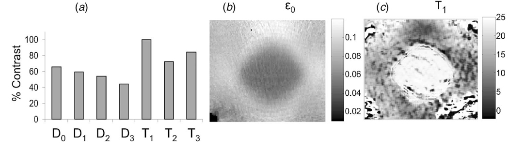
(a) Contrast between 10% and 5.5% homogeneous gelatin samples for seven compliance parameters. (b) Example ϵ₀ image for a composite sample consisting of 5.5% gel background with a 10% gel inclusion. (c) Example T₁ image.

Table 1 shows that viscoelastic amplitudes D₁, D₂, D₃ are at least an order of magnitude lower than the elastic amplitude D₀, and yet the contrasts are quite similar. Assuming E₀ increases with the square of gelatin concentration [44, 45] and D₀=1/E₀, we can estimate D₀ contrast as |(10⁻²–5.5⁻²)/5.5⁻²| =0.69. The estimate is close to the measured value of 0.65 found in Fig. 11(a ). Since D₀ is the largest of the amplitude parameter contrasts and its greater amplitude provides a superior signal-to-noise ratio, D₀ is a good candidate for imaging.

Table 1.

Viscoelastic parameters for 5.5% gelatin acquired by fitting measurements to model functions. First column lists the discrete viscoelastic model order. Second column contains compressive compliance [k Pa⁻¹] and retardance time [s] constants from data of Fig. 12(a). Third column contains wave modulus [k Pa] and relaxation time [s] constants from Fig. 12(b). Fourth column contains shear compliance [k Pa⁻¹] and retardance time constants from Fig. 12(c). Fifth column contains compressive relaxation modulus [k Pa] and relaxation time constants from Fig. 12(d). Q is the probability from χ² goodness-of-fit test.

MO	Fig. 12(a)			Fig. 12(b)			Fig. 12(c)			Fig. 12(d)
2	D0=0.109			M0=307			J0=0.908
	D1=0.005		T1=26.8	M1=47.9		T1=13.7	J1=0.024		T1=9.8	E1=0.46		T1=22
	D2=0.006		T2=338	M2=77.6		T2=198	J2=0.027		T2=69.5	E2=0.47		T2=302
		Q=0			Q=0			Q=0.34			Q=0
3	D0=0.107			M0=307			J0=0.904
	D1=0.004		T1=5.5	M1=65.3		T1=1.5	J1=0.015		T1=2.8	E1=0.36		T1=3.5
	D2=0.004		T2=49.8	M2=38.6		T2=53	J2=0.017		T2=16.0	E2=0.32		T2=40
	D3=0.006		T3=369	M3=61.3		T3=237	J3=0.024		T3=69.7	E3=0.43		T3=310
		Q=0.65			Q=0.48			Q=0.41			Q=0.30

In practice, we image strain ϵ₀(x)=D₀(x)σ_a(x). If σ_a(x)=σ_a is constant throughout the volume, then elastic strain images are proportional to the compliance distribution. However it is well known that stresses in heterogeneous media vary with position [49]. For example, Fig. 11(b) is an ϵ₀ image of a 5.5% gelatin block into which a stiff cylindrical inclusion of 10% gelatin [24] is placed. Strain in the regions surrounding the inclusion vary because the local stresses are nonuniform.

T₁ and either T₂ or T₃, depending on available acquisition times, are also reasonable choices to represent fluid and matrix responses of gelatin. An example T₁ image is shown in Fig. 11(c). Lesion areas are brighter, indicating that mechanisms take longer due to the increased collagen density when compared to softer background areas. ϵ₀, T₁, and T₂ are the three parameters currently used for viscoelastic imaging [46]. The measurements of Fig. 11 should be repeated to select parameters for imaging biological tissues.

3.7 Viscoelastic Spectra

Figure 12 displays Fourier spectra with corresponding respondance time distributions for four experiments. Specifically, we plot D̆(ω) and L̃⁽³⁾(ω) in part (a), M̆(ω) and H̃⁽⁵⁾(ω) in part (b), J̆(ω) and L̃⁽³⁾(ω) in part (c), and Ĕ(ω) and H̃⁽³⁾(ω) in part (d). The notation L̃⁽³⁾ indicates the approximation to Eq. (13) converges at k=3. The Fourier spectral bandwidth in each case is less than 10 rad/s.

Fig. 12.

Normalized Fourier, retardation, and relaxation spectra. (a) Unconfined type A gelatin samples (aged three days) loaded uniaxially at σ_a=860 Pa are measured for 2000 s using Method A. (b) Confined type A gelatin samples (aged 1 day) strained uniaxially at ϵ_a=0.02 are measured for 2500 s using Method B. (c) Type B gelatin samples (aged 1 day) sheared at ${\sigma }_a^{\prime }=3$ Pa are measured for 3000 s in a rheometer using Method C. (d) Unconfined type A gelatin samples (aged three days) strained uniaxially at ϵ_a=0.08 are measured for 2000 s by combining Methods A and B. Arrows indicate frequencies corresponding to the respondance times given in Table 1. Spectral amplitudes are uniformly reduced across the bandwidth as samples age.

Table 1 lists parameters estimated by curve fitting the data in Fig. 12 to model functions. The χ² probabilities in Table 1 show that a third-order model is required for uniaxial compression (Figs. 12(a), 12(b)) to meet the goodness-of-fit criteria for accepting a discrete model representation, i.e., Q > 0.2. In shear, Fig. 12(c), a second-order Voigt model was found sufficient. Respondance times T for acceptable model fits are indicated in the plots by arrows at the corresponding frequencies ω=1/T.

The spectrum of the confined gelatin sample in compression (Fig. 12(b)) is clearly bimodal. The high-frequency spectral peak corresponds to the fastest relaxation time constant, and the low-frequency peak corresponds to the two slowest relaxation times constants.

The spectrum of the unconfined sample in compression (Fig. 12(a)), could be bimodal, however, the poles of the Voigt model appear more uniformly distributed along the log-frequency axis. The spectrum of the sheared sample (Fig. 12(c)), appears unimodal and skewed. The two poles suggest a second-order Voigt model.

Figure 12 increases confidence that creep and stress relaxation spectra may be compared: the creep response of Fig. 12(a) is a very similar to the stress relaxation response of Fig. 12(d). Spectral similarity suggests that relaxation and retardation times are similarly distributed even if response times from the Voigt and Maxwell models may not be easily related.

4 Discussion

These data allow us to address a few fundamental questions regarding elasticity imaging. Can we interpret properties of the polymeric molecular structure from viscoelastic parameters? If so, which parameters are most promising for imaging and how should we measure them? The conclusions apply to biological tissues only if gelatin gels are a reasonable model, which has yet to be tested.

Regarding interpretation, there is a rich literature on molecular theories of polymer dynamics for standard measurement geometries based on spectral data similar to Fig. 12. Ferry [28] shows that relaxation and retardation spectra have two maxima when the molecular weight of weakly cross-linked polymers is greater than a threshold value. We see two broad peaks in gelatin spectra near ω=1 and 0.01. The high-frequency peak may be from frictional forces, i.e., electrostatic and hydrogen bonds, which resist local deformation as polymer fibers are straightened. Short-range movement of collagen molecules in viscous fluids delays the viscoelastic response only a short time as weak bonds reversibly stretch, dissociate, and associate. The low-frequency peak of the bimodal spectra may be from dragging fully extended peptide chains of relatively high molecular weight through the tangled polymer matrix. Ferry refers to this as “entanglement coupling.” Because these movements occur over a large spatial scale, longer response delays are expected.

Tschoegl [23] also addresses the dynamic behavior of weakly cross-linked polymers such as gelatin gels. He refers to it as pseudo-arrheodictic because the frictional forces between matrix fibers that retard strain in creep experiments can appear as delayed fluid flow. When the magnitude of frictional forces varies over time, a portion of the VE response is delayed, which generates a bimodal spectrum. The Ferry and Tschoegl descriptions are consistent if one considers that the time required for fibers to be straightened before they are dragged through the matrix could be the source of the characteristic delay. In that case, spectral peak frequencies are expected to depend on the molecular weight and surface charge density of the matrix fibers. A working hypothesis for biological tissues is that disease states alter properties of the extracellular matrix—the natural polymer of the body—to generate disease-specific contrast in images of viscoelastic parameters.

In both short-duration (fluid) and long-duration (matrix) respondances of gelatin, frictional forces from bending peptide chains and their attraction to the surrounding structured fluids vary in strength given the randomness of the matrix geometry. Thus, there are not two respondance times as expected from discrete modeling but two distributions of times as observed from the spectra of Figs. 12(a), 12(b), and 12(d). The observation that L^(k) and H^(k) were found to converge suggests continuous distributions of respondance times are reasonable to assume.

Confining samples as in Fig. 12(b) forces fluids to flow before the matrix can respond [50]. In the unconfined samples of Figs. 12(a) and 12(d); however, these processes can begin simultaneously. We see from Table 1 that respondance times for the high-frequency peak, i.e., 3.5 and 5.5 s for the unconfined samples, decreases to 1.5 s in the confined sample, while changes in the low-frequency respondances are less pronounced. Sample confinement appears to separate and narrow the distributions, as expected from the Ferry and Tschoegl descriptions.

In shear creep (Fig. 12(c)), tensile forces are applied to the matrix instead of compression. Forces on the matrix fibers near the circumference of the cone-plate are much larger than those near the center of rotation. Consequently, even small rotations engage the matrix immediately. Since polymers resists tensile deformations more than comparable compressive deformations, the larger low-frequency matrix response observed compared to the high-frequency fluid response is expected. Thus, the skewed, unissmodal appearance of the spectrum in Fig. 12(c) may reflect an increased relative weighting of the low-frequency response.

Clearly, low-order discrete viscoelastic models do not provide physical descriptions of polymers. Rather they are parsimonious summaries that help guide selection of imaging parameters. Our burden is to show those parameters are related to essential biological processes. We are concerned that apparently bimodal spectra require third-order discrete models to meet the χ² criteria. At this time, we recommend using spectra to observe the number of modes, and then averaging time constants detected within each mode. For the spectrum of Fig. 12(a), where the χ² criterion suggests a third-order model, we would nevertheless average time constants corresponding to the two lowest-frequency poles and therefore report T₁ = 5.5 s and T₂ = 209.5 s.

Given the interpretation above, it seems that images of elastic strain ϵ₀, and the retardance times T₁ and T₂ form a concise feature space for strain imaging investigations. The frame rate of current ultrasound systems easily provides sufficient temporal resolution to sample the viscoelastic response bandwidth without aliasing. The challenge for viscoelastic parameters is to acquire data over a sufficient time duration to sample the low-frequency spectral response and estimate steady-state viscosity η₀. The longest respondance time for gelatin is less than 400 s, so acquisitions of 800 s are sufficient when η₀ is large. Even though the steady-state viscosity of gelatin is relatively high, it competes with viscoelastic responses and therefore must be eliminated before analyzing the VE response to minimize parameter biases. The threshold for rheodictic strain responses in gelatin is low: less than 30 Pa.

A different approach to viscoelastic modeling that is gaining momentum models the constitutive equation as a fractional derivative [23,51]. Instead of exponential time dependencies, strain retardation (or stress relaxation) is modeled as algebraic decays [52,53]. Mathematically, ϵ_VE(x, t)=D₁(x)𝒟^α{σ(x, t)}, where 𝒟^α is the fractional derivative operator applied to the stimulus and 0 <α<1. The fractional derivative result can form a concise feature representation by the two parameters: D₁(x) and α(x). In fact, [51] shows that there is also a molecular basis for interpreting these parameters in polymer solutions. However, the interpretation in cross-linked polymeric solids with arrheodictic behavior, such as gelatin and soft connective tissues, is still empirical in the sense that α is a characteristic parameter not directly connected to molecular structures.

The creep response in gelatin is well represented by linear viscoelastic theory for applied stresses up to 3 kPa, although the range depends on gel stiffness. The literature for some biological tissues shows a lower threshold for nonlinear responses [21]. The question of interpreting VE parameters for images obtained during large, nonlinear deformations is open [54]. Anecdotal evidence from imaging [17,24] shows there is little change in contrast even for large compressions where nonlinear responses are clearly expected. While interpretation of parameters in terms of polymer structure may require linearity, detection of features in imaging based on contrast may not. In addition, strain errors generated by violations of the linear assumption are relatively small compared with other sources of imaging errors. For example, strain variance increases as ultrasonic echo signals decorrelate during complex motions of heterogeneous media and from echo fields under-sampled with respect to the bandpass of strain gradients [24]. In addition, strain is not directly proportional to compliance when the boundary conditions generate spatially variable local stresses. The generally large object contrast for many biological imaging tasks [4] and the use of Lagrangian coordinates to estimate strain [55] give images of viscoelastic parameters diagnostic value despite violations of assumptions that permit interpretation of results at the molecular scale.

Appendix A: Ramp and Hold Stress Stimulus

Consider the first-order Voigt model in shear, i.e., sJ̃(s) = J₀ +J₁/(1+T₁s), where we assume $t/{\eta }_0^{\prime }~0$ during the measurement time [23]. Let us apply a ramp shear stress σ₁₂(t) = σ_ar(t₀; t₁) over the time interval (t₀, t₁)

$$r(t_0;t_1)=\{\begin{array}{ll}0,\hfill & t\le t_0\hfill \\ t/(t_1-t_0),\hfill & t_0\le t\le {}_1\hfill \\ 1,\hfill & t\ge t_1\hfill \end{array}$$ (24)

In the Laplace domain, σ̃₁₂(s) = (σ_a/(s²t′))[1−e^−t′s], where t′ = t₁−t₀. Combining this information with Eq. (15) and taking the inverse Laplace transform yields shear creep for a ramp stress.

$$\begin{array}{ll}{\gamma }_{12}(t)=\hfill & J_0{\sigma }_a+J_1{\sigma }_a\left[1+\frac{T_1}{t\prime }\text{exp}(-t/T_1)[1-\text{exp}(t\prime /T_1)]\right]\hfill \\ \hfill & \text{for}t\ge t_1\hfill \end{array}$$ (25)

In the limit of t′ → 0, we obtain the response to a step stress γ₁₂(t) = γ₍₁₂₎₀+γ₍₁₂₎₁[1−exp(−t/T₁)]. This can be extended to higher-order models for a linear system via

$$\begin{array}{ll}{\gamma }_{12}(t)=\hfill & {\gamma }_{(12)0}+{\displaystyle \sum _{m=1}^M\frac{{\gamma }_{(12)m}}{t\prime }\{t\prime +T_m\text{exp}(-t/T_m)[1}\hfill \\ \hfill & -\text{exp}(t\prime /T_m)]\}\text{\hspace{1em}for}t\ge t_1\hfill \end{array}$$ (26)

Ramp stimuli reduce the magnitude of viscoelastic responses compared to a step stimulus, particularly at high frequencies, but do not bias retardance time estimates. Results for a compressive ramp stress stimulus yield equivalent effects. For example, Fig. 1(b) compares bimodal spectra simulated with step and 1 s ramp stress stimuli.

Appendix B: Sample Rest Period Analysis

Whenever possible, parameter uncertainty was estimated using data from identical samples measured once each. Measurements were repeated on the same sample only when necessary. We avoided repeated measurements on the same sample because viscoelastic responses are known to depend on deformation history. The following study tests how the rest time allowed between measurements affected estimates.

Figure 13 summarizes the results of a creep experiment conducted on two gelatin samples with identical properties using Method A, where σ_a=733 Pa. Sample I was rested 1 h between the first two measurements and then 2 h between measurements 2 and 3. Sample II was rested 2 h and then 1. Resting 1 h biased retardance times high by as much as a factor of 2. Waiting 2 h reduced biases significantly, although it is clear that the exact deformation sequence is important. It might seem reasonable to recommend 3 or 4-h rests, except that cross-linking also increases over time in gelatin. We recommend keeping the applied load as low as possible and allowing 2-h rests between measurements of 3000 s, or at least twice the acquisition time for shorter duration measurements. Two hour rests are a compromise between the polymeric changes from deformation and those from curing.

Fig. 13.

Effects of rest time on viscoelastic estimates. Top: Variation of T₁ (left group), T₂ (middle group), and T₃ (right group) for a third-order Voigt model are shown for baseline measurements (0) and rest times of 1 and 2 h. Error bars indicate fitting uncertainties. Bottom: Table showing initial baseline retardance times in seconds and percent biases for rest times of 1 or 2 h between measurements.

References

- 1.Fatemi M, Wold L, Alizad A, Greenleaf J. Vibro-Acoustic Tissue Mammography. IEEE Trans. Med. Imaging. 2002;21:1–8. doi: 10.1109/42.981229. [DOI] [PubMed] [Google Scholar]
- 2.Sharma A, Soo M, Trahey G, Nightingale K. Acoustic Radiation Force Impulse Imaging of in vivo Breast Masses. Proc. IEEE Ultrason. Symp. 2004;Vol. 1:728–731. [Google Scholar]
- 3.Sinkus R, Tanter M, Xydeas T, Catheline S, Bercoff J, Fink M. Viscoelastic Shear Properties of in vivo Breast Lesions Measured by MR Elastography. Magn. Reson. Imaging. 2005;23:159–165. doi: 10.1016/j.mri.2004.11.060. [DOI] [PubMed] [Google Scholar]
- 4.Krouskop T, Wheeler T, Kallel F, Garra B, Hall T. Elastic Moduli of Breast and Prostate Tissues Under Compression. Ultrason. Imaging. 1998;20:260–274. doi: 10.1177/016173469802000403. [DOI] [PubMed] [Google Scholar]
- 5.Elenbaas B, Weinberg R. Heterotypic Signaling Between Epithelial Tumor Cells and Fibroblasts in Carcinoma Formation. Exp. Cell Res. 2001;264:169–184. doi: 10.1006/excr.2000.5133. [DOI] [PubMed] [Google Scholar]
- 6.Insana M, Pellot-Barakat C, Sridhar M, Lindfors K. Viscoelastic Imaging of Breast Tumor Microenvironment With Ultrasound. J. Mammary Gland Biol. Neoplasia. 2004;9:393–404. doi: 10.1007/s10911-004-1409-5. [DOI] [PMC free article] [PubMed] [Google Scholar]
- 7.Jin S, Oshinski J, Giddens D. Effects of Wall Motion and Compliance on Flow Patterns in the Ascending Aorta. ASME J. Biomech. Eng. 2003;125:347–354. doi: 10.1115/1.1574332. [DOI] [PubMed] [Google Scholar]
- 8.Zoumi A, Lu X, Kassab G, Tromberg B. Imaging Coronary Artery Microstructure Using Second-Harmonic and Two-Photon Fluorescence Microscopy. Biophys. J. 2004;87:2778–2786. doi: 10.1529/biophysj.104.042887. [DOI] [PMC free article] [PubMed] [Google Scholar]
- 9.Ganten M, Boese J, Leitermann D, Semmler W. Quantification of Aortic Elasticity: Development and Experimental Validation of a Method Using Computed Tomography. Eur. Radiol. 2005;15:2506–2512. doi: 10.1007/s00330-005-2857-z. [DOI] [PubMed] [Google Scholar]
- 10.Zhang X, Kinnick R, Fatemi M, Greenleaf J. Noninvasive Method for Estimating a Complex Elastic Modulus of Arterial Vessels. IEEE Trans. Ultrason. Ferroelectr. Freq. Control. 2005;52:642–652. doi: 10.1109/tuffc.2005.1428047. [DOI] [PubMed] [Google Scholar]
- 11.Zlatanova J, Leuba S. Stretching and Imaging Single DNA Molecules and Chromatin. J. Muscle Res. Cell Motil. 2002;23:377–395. doi: 10.1023/a:1023498120458. [DOI] [PubMed] [Google Scholar]
- 12.Ko H, Tan W, Stack R, Boppart S. Optical Coherence Elastography of Engineered and Developing Tissue. Tissue Eng. 2006;12:63–73. doi: 10.1089/ten.2006.12.63. [DOI] [PubMed] [Google Scholar]
- 13.Ingber D. Tensegrity II. How Structural Networks Influence Cellular Information Processing Networks. J. Cell. Sci. 2003;116:1397–1408. doi: 10.1242/jcs.00360. [DOI] [PubMed] [Google Scholar]
- 14.Weinbaum S, Zhang X, Han Y, Vink H, Cowin S. Mechanotransduction and Flow Across the Endothelial Glycocalyx. Proc. Natl. Acad. Sci. U.S.A. 2003;100:7988–7995. doi: 10.1073/pnas.1332808100. [DOI] [PMC free article] [PubMed] [Google Scholar]
- 15.Garra B, Cespedes E, Ophir J, Spratt S, Zurbier R, Magnant C, Pannanen M. Elastography of Breast Lesions: Initial Clinical Results. Radiology. 1997;202:79–86. doi: 10.1148/radiology.202.1.8988195. [DOI] [PubMed] [Google Scholar]
- 16.McKnight A, Kugel J, Rossman P, Manduca A, Hartmann L, Ehman RL. MR Elastography of Breast Cancer: Preliminary Results. AJR, Am. J. Roentgenol. 2002;178:1411–1417. doi: 10.2214/ajr.178.6.1781411. [DOI] [PubMed] [Google Scholar]
- 17.Pellot-Barakat C, Sridhar M, Lindfors K, Insana M. Ultrasonic Elasticity Imaging as a Tool for Breast Cancer Diagnosis and Research. Current Medical Imaging Reviews. 2006;2:157–164. [Google Scholar]
- 18.Lorenzen J, Sinkus R, Biesterfeldt M, Adam G. Menstrual-Cycle Dependence of Breast Parenchyma Elasticity: Estimation With Magnetic Resonance Elastography of Breast Tissue During the Menstrual Cycle. Invest. Radiol. 2003;38:236–240. doi: 10.1097/01.RLI.0000059544.18910.BD. [DOI] [PubMed] [Google Scholar]
- 19.Insana M, Sridhar M, Liu J, Barakat C. Ultrasonic Mechanical Relaxation Imaging and the, Material Science of Breast Cancer. Proc. IEEE Ultrason. Symp. 2005;Vol. 2:739–742. [Google Scholar]
- 20.Losa G, Alini M. Sulphated Proteoglycans in the Extracellular Matrix of Human Breast Tissues with Infiltrating Carcinoma. Int. J. Cancer. 1993;54:552–557. doi: 10.1002/ijc.2910540406. [DOI] [PubMed] [Google Scholar]
- 21.Fung Y. Biomechanics: Mechanical Properties of Living Tissues. 2nd ed. New York: Springer; 1993. [Google Scholar]
- 22.Wineman A, Rajagopal K. Mechanical Response of Polymers. Cambridge: Cambridge University Press; 2000. [Google Scholar]
- 23.Tschoegl N. Phenomenological Theory of Linear Viscoelastic behavior. New York: Springer; 1989. [Google Scholar]
- 24.Chaturvedi P, Insana M, Hall T. Testing the Limitations of 2-D Companding for Strain Imaging Using Phantoms. IEEE Trans. Ultrason. Ferroelectr. Freq. Control. 1998;45:1022–1031. doi: 10.1109/58.710585. [DOI] [PubMed] [Google Scholar]
- 25.Purslow P, Wess T, Hukins D. Collagen Orientation and Molecular Spacing During Creep and Stress Relaxation in Soft Connective Tissues. J. Exp. Biol. 1998;201:135–142. doi: 10.1242/jeb.201.1.135. [DOI] [PubMed] [Google Scholar]
- 26.Hayes W, Keer L, Herrmann G, Mockros L. Dynamic Study of Gelatin Gels by Creep Measurements. Rheol. Acta. 1997;36:610–617. [Google Scholar]
- 27.Higgs P, Ross-Murphy S. Creep Measurements on Gelatin Gels. Int. J. Biol. Macromol. 1990;12:233–240. doi: 10.1016/0141-8130(90)90002-r. [DOI] [PubMed] [Google Scholar]
- 28.Ferry J. Viscoelastic Properties of Polymers. 3rd ed. New York: John Wiley and Sons; 1980. [Google Scholar]
- 29.ODonnell M, Skovoroda A, Shapo B, Emelianov S. Internal Displacement and Strain Imaging Using Ultrasonic Speckle Tracking. IEEE Trans. Ultrason. Ferroelectr. Freq. Control. 1994;42:314–325. [Google Scholar]
- 30.Ophir J, Cespedes I, Ponnekanti H, Yazdi Y, Li X. Elastography: A Quantitative Method for Imaging the Elasticity of Biological Tissues. Ultrason. Imaging. 1991;13:111–134. doi: 10.1177/016173469101300201. [DOI] [PubMed] [Google Scholar]
- 31.Schwarzl F, Staverman A. Higher Approximation Methods for the Relaxation Spectrum From Static and Dynamic Measurements of Visco-Elastic Materials. Appl. Sci. Res., Sect. A. 1953;4:127–141. [Google Scholar]
- 32.Shung K, Smith M, Tsui B. Principles of Medical Imaging. San Diego: Academic Press, Inc.; 1992. [Google Scholar]
- 33.The loss compliance D̆(ω) (Eq. (10)) for a first-order Voigt model is . The spectrum peaks at ω=1/T1 as found from dD̆(ω)/dω = 0.
- 34.To go from the discrete model of Eq. (6) to a continuous distribution of retardance times, we assume can be written as a uniformly sampled function , where Tℓ=n∆τ for some integer value n. Using sampling theory, . Ds has units [Pas]−1.
- 35.Bot A, van Amerongen I, Groot R, Hoekstra N, Agterof W. Large Deformation Rheology of Gelatin Gels. Polym. Gels Networks. 1996;4:189–227. [Google Scholar]
- 36.Djabourov M, Bonnet N, Kaplan H, Favard N, Favard P, Lechaire J, Maillard M. 3D Analysis of Gelatin Gel Networks From Transmission Electron Microscopy Imaging. J. Phys. II. 1993;3:611–624. [Google Scholar]
- 37.Madsen E, Hobson M, Shi H, Varghese T, Frank G. Tissue-Mimicking Agar/Gelatin Materials for Use in Heterogeneous Elastography Phantoms. Phys. Med. Biol. 2005;50:5597–5618. doi: 10.1088/0031-9155/50/23/013. [DOI] [PMC free article] [PubMed] [Google Scholar]
- 38.Pezron I, Djabourov M. X-ray Diffraction of Gelatin Fibers in the Dry and Swollen States. J. Polym. Sci., Part B: Polym. Phys. 1990;28:1823–1839. [Google Scholar]
- 39.Ward A. The Physical Properties of Gelatin Solutions and Gels. Br. J. Appl. Phys. 1954;5:85–90. [Google Scholar]
- 40.Veis A. The Macromolecular Chemistry of Gelatin. New York: Academic Press; 1964. [Google Scholar]
- 41.Stoeckelhuber M, Stumpf P, Hoefter E, Welsch U. Proteoglycan-Collagen Associations in the Non-lactating Human Breast Connective Tissue During the Menstrual Cycle. Histochem. Cell Biol. 2002;118:221–230. doi: 10.1007/s00418-002-0438-7. [DOI] [PubMed] [Google Scholar]
- 42.Yakimets I, Wellner N, Smith A, Wilson R, Farhat I, Mitchell J. Mechanical Properties With Respect to Water Content of Gelatin Films in Glassy State. Polymer. 2005;46:12577–12585. [Google Scholar]
- 43.Tanzer M. Intermolecular Cross-Links in Reconstituted Collagen Fibrils. J. Biol. Chem. 1968;243:4045–4054. [PubMed] [Google Scholar]
- 44.Hall T, Bilgen M, Insana M, Krouskop T. Phantom Materials for Elastography. IEEE Trans. Ultrason. Ferroelectr. Freq. Control. 1997;44:1355–1365. [Google Scholar]
- 45.Gilsenan P, Ross-Murphy S. Shear Creep of Gelatin Gels From Mammalian and Piscine Collagens. Int. J. Biol. Macromol. 2001;29:53–61. doi: 10.1016/s0141-8130(01)00149-0. [DOI] [PubMed] [Google Scholar]
- 46.Sridhar M, Insana M. Lecture Notes in Computer Science, IPMI 05. Vol. 5373. New York: Springer; 2005. Imaging Microenvironment With Ultrasound; pp. 202–211. [Google Scholar]
- 47.Hayes W, Keer L, Herrmann G, Mockros L. A Mathematical Analysis for Indentation Tests of Articular Cartilage. J. Biomech. 1972;5:541–551. doi: 10.1016/0021-9290(72)90010-3. [DOI] [PubMed] [Google Scholar]
- 48.Press W, Flannery B, Teukolsky S, Vetterling W. Numerical Recipes: The Art of Scientific Computing. New York: Cambridge University Press; 1986. [Google Scholar]
- 49.Bilgen M, Insana M. Elastostatics of a Spherical Inclusion in Homogeneous Biological Media. Phys. Med. Biol. 1998;43:1–20. doi: 10.1088/0031-9155/43/1/001. [DOI] [PubMed] [Google Scholar]
- 50.Knapp D, Barocas V, Moon A. Rheology of Reconstituted Type I Collagen Gel in Confined Compression. J. Rheol. 1997;41:971–993. [Google Scholar]
- 51.Bagley R. A Theoretical Basis for the Application of Fractional Calculus to Viscoelasticity. J. Rheol. 1983;27:201–210. [Google Scholar]
- 52.Ouis D. Characterization of Polymers by Means of a Standard Viscoelastic Model and Fractional Derivate Calculus. Int. J. Polym. Mater. 2004;53:633–644. [Google Scholar]
- 53.Welch S, Rorrer R, Duren R. Application of Time-Based Fractional Calculus Methods to Viscoelastic Creep and Stress Relaxation of Materials. Mech. Time-Depend. Mater. 1999;3:279–303. [Google Scholar]
- 54.Samani A, Plewes D. A Method to Measure the Hyperelastic Parameters of ex vivo Breast Tissue Samples. Phys. Med. Biol. 2004;49:4395–4405. doi: 10.1088/0031-9155/49/18/014. [DOI] [PubMed] [Google Scholar]
- 55.Maurice R, Bertrand M. Lagrangian Speckle Model and Tissue-Motion Estimation-Theory. IEEE Trans. Med. Imaging. 1999;18:593–603. doi: 10.1109/42.790459. [DOI] [PubMed] [Google Scholar]