Efficient Algorithms to Explore Conformation Spaces of Flexible Protein Loops

Abstract

Several applications in biology—e.g., incorporation of protein flexibility in ligand docking algorithms, interpretation of fuzzy X-ray crystallographic data, and homology modeling—require computing the internal parameters of a flexible fragment (usually, a loop) of a protein in order to connect its termini to the rest of the protein without causing any steric clash inside the loop and with the rest of the protein. One must often sample many such conformations in order to explore and adequately represent the conformational range of the studied loop. While sampling must be fast, it is made difficult by the fact that two conflicting constraints—kinematic closure and clash avoidance—must be satisfied concurrently. This paper describes two efficient and complementary sampling algorithms to explore the space of closed clash-free conformations of a flexible protein loop. The “seed sampling” algorithm samples broadly from this space, while the “deformation sampling” algorithm uses seed conformations as starting points to explore the conformation space around them at a finer grain. Computational results are presented for various loops ranging from 5 to 25 residues. More specific results also show that the combination of the sampling algorithms with a functional site prediction software (FEATURE) makes it possible to compute and recognize calcium-binding loop conformations. The sampling algorithms are implemented in a toolkit, called LoopTK, which is available at https://simtk.org/home/looptk.

1 INTRODUCTION

Several applications in biology require exploring the conformation space of a flexible fragment (usually, a loop) of a protein. For example, upon binding with a small ligand, a fragment may undergo deformations to rearrange nonlocal contacts [23]. Incorporating such flexibility in docking algorithms is a major challenge [26]. In X-ray crystallography experiments, electron density maps (EDMs) often contain noisy regions caused by disorder in the crystalline sample, resulting in an initial model with missing fragments between resolved termini [28]. Similarly, in homology modeling [24], only parts of a protein structure can be reliably inferred from known structures with similar sequences. These applications share a common subproblem: to compute closed, clash-free conformations of an inner fragment of a protein chain. These conformations lie in a complex subset of the fragment’s conformation space.

This problem requires satisfying two constraints concurrently: closing a kinematic loop and avoiding steric clashes. Each constraint considered separately is relatively easy to satisfy, but the combination is hard because the two constraints are conflicting. The closed conformations of a loop with n degrees of freedom (DOFs)—e.g., n dihedral angles ϕ and ψ—form a subspace of dimensionality at least n − 6 contained in the n-dimensional conformation space of the loop. Due to protein compactness, the conformations that are both closed and clash-free typically form a subset of this subspace that has a very small relative volume, especially for long loops. Hence, an arbitrary closed conformation of the loop has small probability to be clash-free. Conversely, an arbitrary collision-free conformation of the loop has null probability to be closed. As a result, existing sampling techniques often have high rejection ratios.

In this paper, we present two new techniques, seed and deformation sampling, to solve this problem. Each deformation sampling operation starts from a given closed clash-free conformation (a “seed”) and deforms this conformation without breaking closure or introducing clashes by modifying the loop’s DOFs in a coordinated way. In contrast, seed sampling generates new conformations from scratch, by prioritizing the treatment of the two constraints, so that the most limiting one is enforced first. In both techniques, prevention and detection of steric clashes is done using the grid-indexing method described in [17]. Seed and deformation sampling complement each other very well. Seed sampling produces conformations that are broadly distributed over the loop’s conformation space and provides conformations (seeds) later used by deformation sampling to explore more finely certain regions of this space. These algorithms are implemented into a toolkit, LoopTK, available at https://simtk.org/home/ looptk. They have been tested on various loops ranging from 5 to 25 residues.

Section 2 compares our work to motivation and previous work. Section 3 outlines the loop kinematic model used in this paper. Sections 4 and 5 describe the seed and deformation sampling algorithms, respectively. Section 6 briefly presents the grid technique used both to detect steric clashes and to identify pairs of close atoms. Section 7 discusses various results obtained with the implemented software. In particular, Section 7.4 shows that the combination of our algorithms with FEATURE (a functional site prediction software) [31] makes it possible to compute calcium-binding loop conformations.

2 MOTIVATION AND PREVIOUS WORK

The problem considered in this paper is a version of the “loop closure” problem studied in [5], [10], [12], [18], [21], and [30]. Several works have specifically focused on kinematic closure. Analytical Inverse Kinematics (IK) methods are described in [10] and [30] to close a fragment of three residues. For longer fragments, iterative techniques have been proposed, like the popular Cyclic Coordinate Descent (CCD) [5] and the “null space” technique [25], [28]. We reuse several of these techniques in our work. In particular, our seed sampling algorithm applies the analytical IK method described in [10] in a new way to close loops with more than three residues. Our deformation sampling algorithm uses the null space technique to deform loops without breaking closure.

Procedures to sample closed clash-free conformations of loops by varying dihedral angles have been proposed in [9], [12], and [18]. The goal of RAPPER [12] and the hierarchical method described in [18] is to generate near-native conformations by minimizing an energy function. Instead, the goal of our method and the one presented in [9] is to explore the closed clash-free conformation space of a loop by sampling conformations broadly distributed across this space. This ability to explore a conformation space is critical for a number of applications. For example, the conformation selection theory [3] suggests that a protein and a ligand exist in an ensemble of deforming folded conformations and that the most compatible conformations “recognize” each other and bind together. Binding conformations of proteins often differ significantly from native ones. To predict protein function, one must be able to sample these nonnative but biologically relevant conformations. As another example, an EDM obtained from an X-ray crystallographic experiment can be particularly difficult to interpret when the protein appears in the crystalline sample in multiple states. An ensemble of sampled conformations may then be needed to provide a satisfactory interpretation of the EDM [14], [22]. Nevertheless, our deformation sampling technique also allows energy minimization, when this is desirable. We show in Section 7.4 that our seed and deformation sampling procedures can generate biologically important conformations.

RAPPER [12] iteratively generates a loop conformation from its N terminus toward its C terminus by selecting the values of the dihedral angles ϕ and ψ at random from a predefined discrete table of values. It also checks that the Cα atom in each residue is sufficiently close to the loop’s C anchor on the protein. In the end, to close the gap between the loop’s last residue and its anchor on the protein, RAPPER runs an iterative minimization procedure to reduce this gap. Unlike RAPPER, our method does not select dihedral angles from discrete tables but picks them according to probability distributions input by the user. In addition, our method retains a sufficient number of dihedral angles (in the middle portion of the loop) to make it possible to close the loop using an exact IK method.

Like our seed sampling method, the method presented in [18] also exploits the idea of loop decomposition. It breaks a loop into two fragments, then independently sample clash-free conformations for each fragment (by sampling dihedral angles starting from their respective anchors) and, finally, generates closed conformations by bridging close-enough fragment conformations. Like RAPPER, this method selects dihedral angles from predefined discrete tables. It uses IK and steric clash techniques that are very different from ours. Both RAPPER and this method have been tested on relatively short loops having between 2 and 12 residues in length.

The Random Loop Generator (RLG) method described in [9] is used to study the potential mobility of a loop in the presence and absence of certain side chains. It successively samples closed conformations that it later tests for steric clashes. To sample closed conformations, it divides the loop backbone into “active” and “passive” fragments. The latter has exactly three residues (hence, six dihedral angles). The dihedral angles in the active fragment are successively sampled at random using a geometric algorithm that increases the likelihood that a closed conformation will eventually be obtained. The six dihedral angles of the passive fragment are used to close the loop using an IK procedure. The generated closed conformations are then tested for steric clashes. To explore the conformation space of the loop, a tree of sampled conformations is built starting from a known structure (typically, the native structure), the root of the tree. Each node of the tree is a conformation generated using RLG in a neighborhood of its parent in the tree. Our deformation sampling, which also generates each new conformation in the neighborhood of an already sampled conformation, has similarities with this method. However, unlike RLG, our method perturbs the dihedral angles in such a way that it does not break closure.

Some sampling procedures try to sample conformations using libraries of fragments obtained from previously solved structures [11], [21], [27], [29]. For example, a divide-and-conquer approach is described in [27] that generates a database of fragments of different residue lengths and types, by using a Ramachandran plot distribution. These fragments are then concatenated to build conformations of a longer loop. However, steric clashes are not taken into account during this process. Other works sample loop conformations directly by minimizing an energy function [2], [12], [13], [18], [25] or running a molecular dynamics simulation [4] with the goal to identify loop fragments close to native structure. However, as discussed above, in a number of applications it is preferable to explore the closed clash-free conformation space of a loop.

In our algorithms, steric clash detection is done using the efficient grid method previously described in [17]. A similar detection method is also used in RAPPER [12].

3 LOOP MODEL

A loop L is defined here as a sequence of p > 3 consecutive residues in a protein P, such that none of the two termini of L is also a terminus of P.We number the residues of L from 1 to p, starting from the N terminus. We model the backbone of L as a serial linkage whose DOFs are the n = 2p dihedral angles ϕ_i and ψ_i around the bonds N−Cα and Cα−C, in residues i = 1,…,p. The rest of the protein, denoted by P \ L, is assumed rigid. We let L_B denote the backbone of L. It includes the Cβ and O atoms, respectively, bonded to the Cα and C atoms in the backbone.

We attach a Cartesian coordinate frame Ω₁ to the N terminus of L and another frame Ω₂ to its C terminus. When L_B is connected to its anchors in the rest of the protein, i.e., when it adopts a closed conformation, the pose (position and orientation) of Ω₂ relative to Ω₁ is fixed to a predefined value that we denote by Π_g.

If we arbitrarily pick the values of ϕ_i and ψ_i, i = 1 to p, then in general we get an open conformation of L_B, where the pose of Ω₂ relative to Ω₁ differs from Π_g. The set Q of all open and closed conformations of L_B is a space of dimensionality n = 2p. The subset Q_closed of closed conformations is a subspace of Q of dimensionality at least n − 6. Let Π(q) denote the pose of Ω₂ relative to Ω₁ when the conformation of L_B is q ∈ Q. The function Π and its inverse Π⁻¹ are the “forward” and “inverse” kinematics map of L_B, respectively.

A conformation of L_B is clash-free if and only if no two atoms, one in L_B, the other in L_B or P \ L, are such that their centers are closer than ε times the sum of their van der Waals radii, where ε is a constant in (0, 1). In our software, ε is an adjustable parameter, usually set to 0.75, which approximately corresponds to the distance where the van der Waals potential associated with two atoms begins increasing steeply. We denote the set of closed clash-free conformations of L_B by ${\mathrm{Q}}_{\text{closed}}^{\text{free}}$ . In general, it has the same dimensionality as Q_closed, but its volume is usually a small fraction of that of Q_closed.

4 SEED SAMPLING

4.1 Overview

The goal of seed sampling is to generate conformations of L_B broadly distributed over ${\mathrm{Q}}_{\text{closed}}^{\text{free}}$ . The challenge comes from the interaction between the kinematic closure and clash avoidance constraints. Computational tests (see Section 7) show that the approach (hereafter called the naive approach) that first samples conformations from Q_closed and next rejects those with steric clashes is often too time consuming, except for short loops, due to its huge rejection ratio. The reverse approach—sampling the angles ϕ_i and ψ_i of L_B to avoid clashes—will inevitably end up with open conformations, since Q_closed has lower dimensionality than Q.

These insights led us to develop a prioritized constraint-satisfaction approach, hereafter called the prioritized approach. We partition L_B into three segments, the front-end F, the mid-portion M, and the back-end B. F starts at the N terminus of L_B and B ends at its C terminus. M is the segment between them. Due to the immediate proximity of atoms in P \ L, the conformations of F and B are more limited by the clash avoidance constraint than by the closure constraint; so, we sample the dihedral angles in F and B to avoid clashes, ignoring the closure constraint. Then, for any pair of conformations of F and B, the possible conformations of M are mainly limited by the closure constraint; so, we use the naive approach to sample conformations of M, by running an IK procedure to close the gap between F and B and testing the clash avoidance constraint afterward. In this way, our prioritized approach reduces the application of the naive approach to a short fragment of the loop. The length of M must be large enough for the IK procedure to succeed with high probability but not too large since clash avoidance is only tested afterward. In our software, the number of residues in M is usually set to half of that of L_B or to 4, whichever of these two numbers is larger. The number of residues of F and B are then selected equal (± 1). Tests show that these choices are close to optimal on average for a wide range of loops. For unusually long loops, it may be suitable to set an upper bound on the length of M.

The dihedral angles ϕ and ψ in the three fragments F, M, and B are selected to generate conformations of L_B broadly distributed over ${\mathrm{Q}}_{\text{closed}}^{\text{free}}$ .

4.2 Sampling Front/Back-End Conformations

Consider the front-end F. The angles ϕ and ψ closest to the fixed terminus of F are the most constrained by possible clashes with the rest of the protein P \ L. So, the angles are sampled in the order in which they appear in F, that is, ϕ₁, ψ₁, ϕ₂, and so forth. In this order, each angle ϕ_i (respectively, ψ_i) determines the positions of the next two atoms C_{β i} and C_i (respectively, the next three atoms O_i, N_i+1, and Cα_i+1). The angle is sampled so that these atoms do not clash with any atom in P \ L or any preceding atom in F. Its value is picked at random, either uniformly or according to a user-input probabilistic distribution (e.g., one based on Ramachandran tables). If no value of the angle prevents the two or three atoms it governs from clashing with other atoms, the algorithm backtracks and resamples a previously sampled angle. Clash-free conformations of the back-end B are sampled in the same way, by starting from its fixed C terminus and proceeding backward.

4.3 Sampling Mid-Portion Conformations

Given two nonclashing conformations of F and B such that the gap between them does not exceed the maximal length that M can achieve, a conformation of M is sampled as follows:

The values of the ϕ and ψ angles in M are picked at random, uniformly, or according to a given distribution. This leads to a conformation q of M that is connected to F at one end and open at the other end. To close the gap between M and B, we use the IK method described in [10]. This method solves the IK problem analytically, for any sequence of residues in which exactly three pairs of (ϕ, ψ) dihedral angles are allowed to vary. These pairs need not be consecutive.

Let us denote the IK method by ANALYTICAL-IK(q, i, j, k), where argument q is the initial open conformation of M and arguments i, j, and k are the integers identifying the three residues that contain the pairs of dihedral angles that are allowed to vary. Our experiments show that, on average, the IK method is the most likely to succeed in closing the gap when one pair is the last one in M and the other two are distributed in M. Let r and s denote the integers identifying the first and last residues of M in L_B. As the IK method is extremely fast, ANALYTICAL-IK(q, i, j, s) is called for all i = r,…, s − 2 and j = i + 1,…, s − 1, in a random order, until a closed conformation of M has been generated. If this conformation tests clash-free, then the seed sampling procedure constructs a closed clash-free conformation of L_B by concatenating the conformations of F, M, and B.

If the above operations fail to generate a closed clash-free conformation of M, then they are repeated (with new initial values for the ϕ and ψ angles in M) until a predefined maximal number of iterations have been performed.

We have also experimented with iterative IK techniques, like CCD, to close the gap between M and B. In our implementation, they were slower than the above algorithm based on analytical IK.

4.4 Placing Side Chains

For each conformation of L_B sampled from ${\mathrm{Q}}_{\text{closed}}^{\text{free}}$ , we use SCWRL3 [6] to place the side chains. We may only compute the placements of the side chains in L_B given the placements of the side chains in P \ L. Alternatively, we may (re-)compute the placements of all the side chains in the protein. In each case, SCWRL3 minimizes an energy function that contains volume-exclusion terms. But, it does not fully guarantee that the conformations of the side chains will be clash-free. If needed, we can use deformation sampling to slightly deform the conformation of L_B in order to eliminate the steric clashes (see Section 7.3).

5 DEFORMATION SAMPLING

5.1 Overview

The deformation sampling procedure is given a “seed” conformation q in ${\mathrm{Q}}_{\text{closed}}^{\text{free}}$ . It first selects a vector in the tangent space TQ_closed(q) of Q_closed at q. By definition, any vector in this space is a velocity vector [ϕ̇₁,…,ψ̇_n]^T that maps to the null velocity of Ω₂ (relative to Ω₁); hence, it defines a direction of motion that does not instantaneously break loop closure. A new conformation of L_B is then computed as q′ = q + δq, where δq is a short vector in TQ_closed(q). Since the tangent space is only a local linear approximation of Q_closed at q, the closure constraint is in fact slightly broken at q′. So, ANALYTICAL-IK(q′, p − 2, p − 1, p) is called to bring back the frame Ω₂ to its goal pose Π_g. Since q′ is already almost closed, the six DOFs used by ANALYTICAL-IK are the angles ϕ_p−2,…, ψ_p corresponding to the last three residues of L_B (recall that n = 2p). If ANALYTICAL-IK generates several solutions for these angles, the closest values from those in q + δq are selected. Finally, the atoms in L_B are tested for clashes among themselves and with the rest of the protein. If a clash is detected, the procedure exits with failure.

The deformation sampling procedure may be run several times with the same seed conformation q to explore the subset of ${\mathrm{Q}}_{\text{closed}}^{\text{free}}$ around q. Alternatively, each run may use the conformation generated at the previous run as the new seed to generate a “pathway” in the set ${\mathrm{Q}}_{\text{closed}}^{\text{free}}$ . More generally, one may also build a tree of pathways rooted at a seed conformation or a forest of trees rooted at multiple seeds, e.g., to optimize an objective function.

5.2 Computation of a Basis of the Tangent Space

To define a direction in TQ_closed(q), we must first compute a basis for this space. This can be done as follows [28]: Let J(q) be the 6 × n Jacobian matrix that maps the velocity q̇ = [ϕ̇₁,…, ψ̇_p]^T of the dihedral angles in L_B at q to the velocity [ẋ, ẏ, ż, α̇, β̇, γ̇]^T of Ω₂, i.e., [ẋ, ẏ, ż, α̇, β̇, γ̇]^T = J(q)q̇. J(q) can be computed analytically using techniques presented in [8]. For simplicity, assume that J has full rank (i.e., 6). A basis of TQ_closed(q) is built by first computing the Singular Value Decomposition (UΣV^T) of J(q), where U is a 6 × 6 unitary matrix, Σ is a 6 × n matrix with nonnegative numbers on the diagonal and zeros off the diagonal, and V is an n × n unitary matrix [16]. Since the rows 6,…, n of V do not affect the product J(q)q̇, their transposes form an orthogonal basis N(q) of TQ_closed(q).

5.3 Selection of a Direction in the Tangent Space

The deformation sampling procedure may select a direction in TQ_closed(q) at random. However, in most cases, it is preferable to minimize an objective function E(q). Let y = −∇E(q) be the negated gradient of E at q and y_N = NN^T_y the projection of y into TQ_closed(q). The deformation sampling procedure selects the increment δq along y_N. In this way, all the DOFs left available in L_B by the closure constraints are used to move the conformation in the direction that most reduces E.

E(q) may be a function of the distances between the closest pairs of atoms at conformation q (where each pair consists of one atom in L_B and one atom in either L \ B or L_B). These pairs can be efficiently computed by the same grid method that is used to detect steric clashes (Section 6). Minimizing E then leads deformation sampling to increase the distances between these pairs of atoms, if this goal does not conflict with the closure constraint. In this way, deformation sampling picks increments δ_q that have small risk of causing steric clashes.

Another interesting objective function leads to moving a designated atom A in L_B toward a desired position x_d. This objective function can be defined as

$$E(q)={\Vert x_A(q)-x_d\Vert }^2,$$ (1)

where x_A(q) is the position of A when L_B’s conformation is q. This function can be used to iteratively move an atom as far as possible along selected directions to explore the boundary of ${\mathrm{Q}}_{\text{closed}}^{\text{free}}$ . E can also be an energy function or any weighted combination of functions, each designed to achieve a distinct purpose.

5.4 Placing Side Chains

For each new conformation of L_B, side chains can be placed using SCWRL3, as described in Section 4. Another possibility is to provide an initial seed conformation that already contains the loop’s side chains to the deformation sampling procedure. These side chains are then considered rigid and the procedure deforms L_B so that the produced conformation remains clash-free.

6 STERIC CLASH DETECTION

Steric clash detection is done using the grid method [17]. This method takes advantage of the fact that, to avoid clashes, atoms must spread out, so that any square box of a fixed volume contains an upper bounded number of atom centers, independent of the total number of atoms in the protein.

The method tessellates the 3D space of the protein into an array of equally sized cubes. The edge length of a cube is chosen approximately equal to the largest diameter of the atoms. For a given conformation of the protein, each atom is indexed in the cube that contains its center. Whenever the position of an atom is modified, the grid structure is updated accordingly in constant time. The grid is implemented as a memory-efficient hash table. Only the grid cubes that contain atom centers are represented, each with the corresponding list of atoms.

The clash detection algorithm iterates through all atoms that need to be checked (e.g., the atoms in L_B), asking for each atom if it is in collision. The atom only needs to be checked with the atoms indexed in its own grid cube and the 26 cubes surrounding it. Since the cubes of the grid are small, there are at most four atom centers within one cube. The number of pairs of atoms to check is thus upper bounded by a constant. In practice, the number of checks for each atom is even smaller and usually less than 6. That is, clash detection for a single atom runs in 𝒪(1) time, and the clash test for all 𝒪 (n) atoms in L_B or L runs in 𝒪 (n) time, independent of the total number of atoms in the protein. The same algorithm can be used to find the k closest atoms to a given atom (for a small value of k), simply by considering another layer of grid cubes. This ability allows us to efficiently compute objective functions E, like the one in (1) that contains terms aimed at preventing deformation sampling from producing conformations with steric clashes (Section 5.3).

7 RESULTS

7.1 Seed Sampling

Table 1 lists 20 loops, whose sizes range from 5 to 25 residues, which we used to perform computational tests. Each row lists the PDB ID of the protein, the number of residues in the protein, the number identifying the first residue in the loop, the number of residues in the loop, and the average time to sample one closed clash-free conformation of the loop using two distinct procedures (our seed sampling method and the “naive” method outlined in Section 4.1). In some loops, the two termini are close, while in others they are quite distant. Some loops protrude from the proteins and have much empty space in which they can deform without clash (e.g., 3SEB), while others are very constrained by the other protein residues (e.g., 1TIB). The loop in 1MPP is constrained in the middle by side chains protruding from the rest of the protein (see Fig. 2b). In the results presented below, all ϕ and ψ angles were picked uniformly at random (i.e., no biased distributions, like the Ramachandran’s ones, were used).

Table 1.

Test Set of 20 Loops (See Main Text for Comments)

Protein		Loop		Sampling
Id	Size	Start	Size	Seed	Naive
1XNB	185	SER 31	5	0.22	0.21
1TYS	264	THR 103	5	0.06	0.06
1GPR	158	SER 74	6	0.38	0.38
1K8U	89	GLU 23	7	0.21	0.20
2DRI	271	GLN 130	7	0.42	0.46
1TIB	269	GLY 172	8	2.49	13.03
1PRN	289	ASN 215	8	0.33	0.66
1MPP	325	ILE 214	9	0.53	99.85
4ENL	436	LEU 136	9	1.46	19.35
135L	129	ASN 65	9	0.77	1.54
3SEB	238	HIS 121	10	0.50	3.80
1NLS	237	ASN 216	11	1.30	5.51
1ONC	103	MET 23	11	2.26	5.66
1COA	64	VAL 53	12	19.02	67.49
1TFE	142	GLU 158	12	0.48	8.14
8DFR	186	SER 59	13	2.02	39.36
1THW	207	CYS 177	14	1.48	9.84
1BYI	224	GLU 115	16	2.52	>800
1G5A	628	GLY 433	17	3.28	>800
1HML	123	GLY 51	25	17.74	>800

Fig. 2.

Positions of the middle Cα atom (red dots) in 100 loop conformations computed by seed sampling for four proteins: 1K8U, 1MPP, 1COA, and 1G5A. (a) 1K8U 7-residue loop. (b) 1MPP 9-residue loop. (c) 1COA 12-residue loop. (d) 1G5A 17-residue loop.

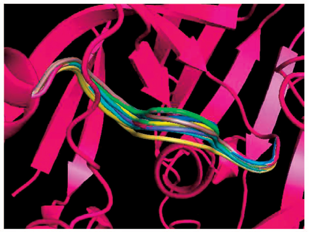
Each picture in Fig. 1 displays a subset of backbone conformations generated by seed sampling for the loops in 1TIB, 3SEB, 8DFR, and 1THW. The loop in 1TIB, which resides at the middle of the protein, has very small empty space to move in. The PDB conformation of the loop in 1THW (shown in green in the picture) bends to the right, but our method also found clash-free conformations that are very different. Each picture in Fig. 2 shows the distributions of the middle Cα atom in 100 sampled conformations of the loops in proteins 1K8U, 1MPP, 1COA, and 1G5A along with a few backbone conformations. The loops in 1K8U and 1COA have relatively large empty space to move in, whereas the loops in 1MPP and 1G5A are restricted by the surrounding protein residues. These figures illustrate the ability of our seed sampling procedure to generate conformations broadly distributed across the closed clash-free conformation space of a loop.

Fig. 1.

Some backbone conformations generated by seed sampling for the loops in 1TIB, 3SEB, 8DFR, and 1THW. (a) 1TIB 8-residue loop. (b) 3SEB 10-residue loop. (c) 8DFR 13-residue loop. (d) 1THW 14-residue loop.

The average running time (in seconds) of our seed sampling procedure to compute one closed clash-free conformation of each loop is shown in column 5 of Table 1. Each average was obtained by running the procedure until it generated 100 conformations of the given loop and dividing the total running time by 100.¹ The last column of Table 1 gives the average running time of the “naive” procedure that first samples closed conformations of the loop backbone and next rejects those which are not clash-free. In both procedures, the factor ε used to define steric clashes (see Section 3) was set to 0.75. Our seed sampling procedure does not break a loop into three segments if it has fewer than eight residues. So, the running times of both procedures for the first five proteins are essentially the same. For all other proteins, our procedure is faster, sometimes by a large factor (188 times faster for the highly constrained loop in 1MPP) than the naive procedure. For the last three proteins, this latter procedure failed to sample 100 conformations after running for more than 80,000 seconds.

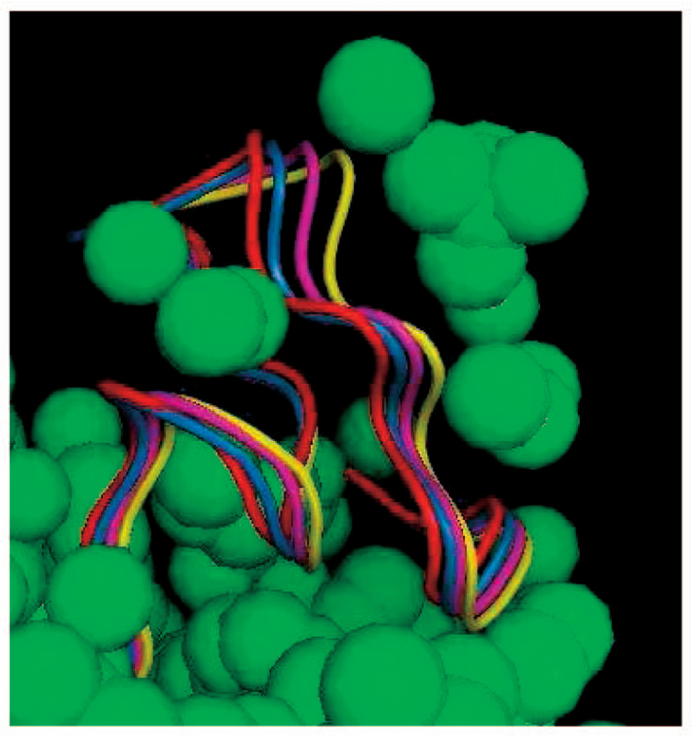
Not surprisingly, the running times vary significantly across loops. Short loops with much empty space around them take a few 1/10 s to sample, while long loops with little empty space can take a few seconds to sample. The loops in 1COA and 1HML take significantly more time to sample than the others. In the case of 1COA, it is difficult to connect the loop’s front end and back end (three residues each) with its mid-portion (six residues). As Fig. 6 shows, the termini of the loop are far apart and the protein constrains the loop all along. Due to the local shape of the protein at the two termini of the loop, many sampled front ends and back ends tend to point in opposite directions, which then makes it often impossible to close the mid-portion without clashes. In this case, we got a better average running time (4 s, instead of 19) by setting the length of the mid-portion to 8 (instead of 6). The loop in 1HML is inherently difficult to sample. Not only is it long, but there is also little empty space available for it. See Fig. 3, where the red conformation of the loop was obtained from the PDB and the other three conformations were sampled by deformation sampling. Other experiments not reported here indicate that the running times reported in Table 1 vary moderately when parameters like the factor ε and the number of residues in the loop’s mid-portion M are slightly modified.

Fig. 6.

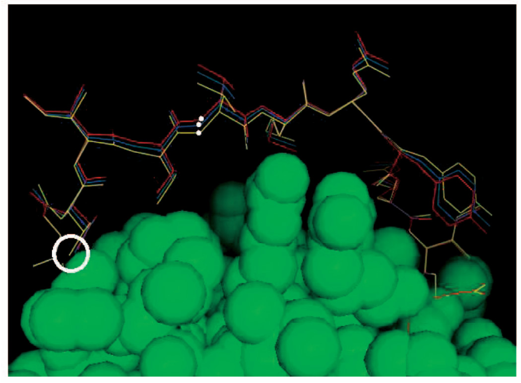
Deformation of the loop in 1COA by pulling the N atom (white dot) of THR 58 along a specified direction.

Fig. 3.

Conformations of the loop in 1HML.

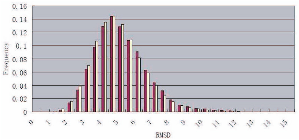
Fig. 4 displays RMSD histograms generated for the loop in 3SEB. The purple (respectively, white) histogram was obtained by sampling 100 (respectively 1,000) conformations of the corresponding loop and plotting the frequency of the RMSDs between all pairs of conformations. The almost identity of the two histograms indicates that the sampled conformations spread quickly in ${\mathrm{Q}}_{\text{closed}}^{\text{free}}$ . Similar histograms were generated for other loops.

Fig. 4.

RMSD histograms for one 10-residue loop in protein 3SEB. The purple color shows the pairwise RMSD distribution of 100 seeds, while the white color shows that of 1,000 seeds.

For rather long loops, any seed sampling procedure that samples broadly ${\mathrm{Q}}_{\text{closed}}^{\text{free}}$ can only produce a coarse distribution of samples. Indeed, for a loop with n dihedral angles, a set of N evenly distributed conformations defines a grid with N^1/n−6 discretized values for each of the n − 6 dimensions of ${\mathrm{Q}}_{\text{closed}}^{\text{free}}$ . If n = 18 (nine-residue loop), a grid with three discretized values per axis requires sampling 531,441 conformations. Deformation sampling makes it possible to sample more densely “interesting” regions of ${\mathrm{Q}}_{\text{closed}}^{\text{free}}$ .

7.2 Deformation Sampling

FIG. 5 shows 20 conformations of the loop in 1MPP generated by deformation sampling around a conformation computed by seed sampling. To produce each conformation, the deformation sampling procedure started from the same seed conformation and selected a short vector δq in TQ_closed(q) at random. This figure illustrates the ability of deformation sampling to explore ${\mathrm{Q}}_{\text{closed}}^{\text{free}}$ around a given conformation.

Fig. 5.

Twenty conformations of the loop in 1MPP generated by deforming a given seed conformation along randomly picked directions.

Fig. 6 shows a series of closed clash-free conformations of the loop in 1COA successively sampled by pulling the N atom (shown as a white dot) of THR 58 away from its initial position along a given direction until a steric clash occurs (white circle). The initial conformation shown in red was generated by seed sampling and the side chains were placed without clashes using SCWRL3. Each other conformation was sampled by deformation sampling starting at the previously sampled conformation and using the objective function E defined by (1). Only the backbone was deformed, and each side chain remained rigid. Steric clashes were tested for all atoms in the loop.

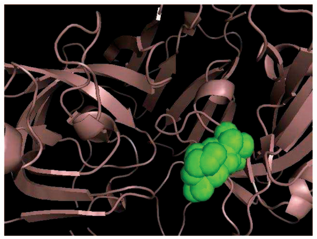
Fig. 7 shows (in green) an approximation of the volume reachable by the fifth Cα atom in the loop of 1MPP. This approximation was obtained by sampling 20 seed conformations of the loop and, for each of these conformations, pulling the fifth Cα atom along several randomly picked directions until a clash occurs. The volume shown in green was obtained by rendering the atom at all the positions it reached.

Fig. 7.

Volume reachable by the fifth Cα atom in the loop of 1MPP.

The running time of deformation sampling depends on the objective function. In the above experiments, it is less than 0.5 second per sample on average.

7.3 Placements of Side Chains

Our software calls SCWRL3 [6] to place side chains. The result, however, is not guaranteed to be clash-free. To generate Table 2, we first ran our seed sampling procedure to sample conformations of the backbones of the loops in 1K8U, 2DRI, 1TIB, 1MPP, and 135L, with the uniform and Ramachandran sampling distributions for the dihedral angles (see Sections 4.2 and 4.3). For each loop, we sampled 50 conformations with the uniform distribution and 50 with the Ramachandran distribution. We then ran SCWRL3 to place side chains in the loop (with the side chains in the rest of the protein fixed) and checked each conformation for steric clashes. Table 2 reports the number of clash-free conformations (out of 50) for each loop. As expected, the backbone conformations generated using the Ramachandran distribution facilitate the clash-free placement of the side chains.

Table 2.

Number of Clash-Free Placements of Side Chains for Five Loops

Protein	1K8U	2DRI	1TIB	1MPP	135L
Uniform	7	9	1	0	9
Ramachandran plots	18	14	6	4	13

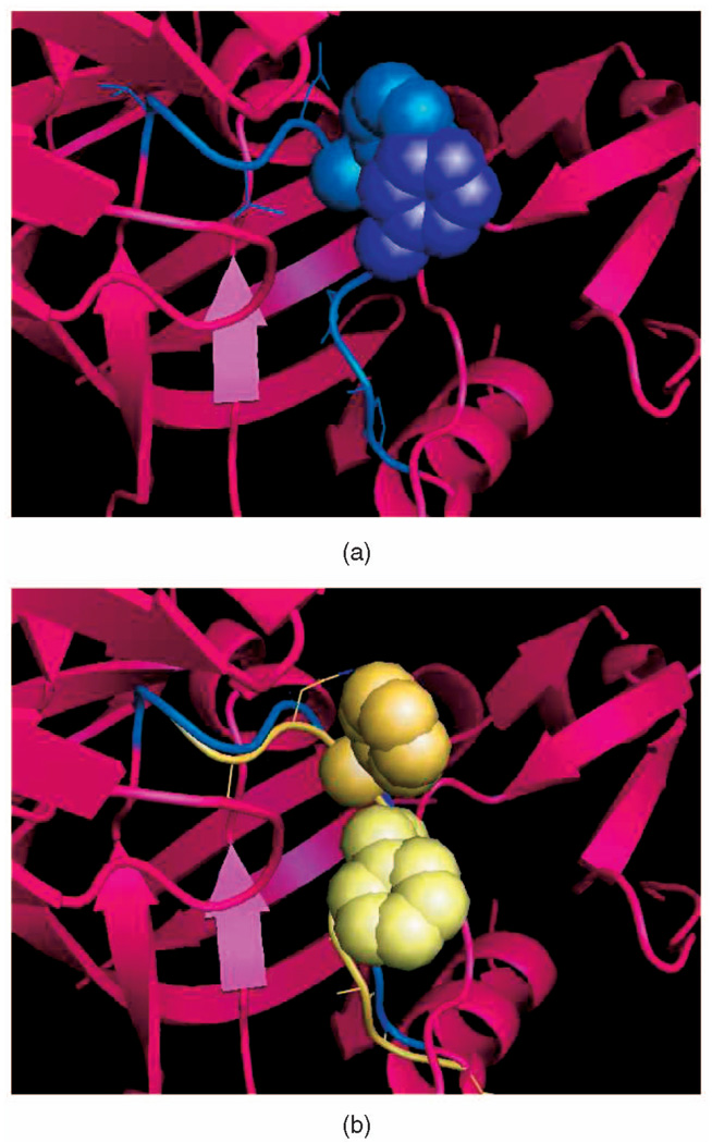
When seed sampling generates a conformation q of a loop backbone, such that SCWRL3 computes a side chain placement that is not clash-free, deformation sampling can then be used to sample more conformations around q, to produce one where side chains are placed without clashes. In Fig. 8a, a conformation (shown in blue) of the backbone of the loop in 1MPP was generated using seed sampling and the side chains were placed by SCWRL3. However, there are clashes between two side chains. In Fig. 8b, a conformation (shown in yellow) was generated by the deformation sampling procedure using the conformation shown in Fig. 8a as the start conformation. The new placement of the side chains computed by SCWRL3 is free of clashes. Once such a clash-free conformation has been obtained, many other clash-free conformations can be quickly generated around it, again using deformation sampling, as shown in Fig. 5.

Fig. 8.

Use of deformation sampling to remove steric clashes involving side chains.

7.4 Calcium-Binding Site Prediction

Calcium-binding proteins play a key role in signal transduction. Many such proteins share the same functional domain, a helix-turn-helix structural motif called EF-hand [20]; the calcium ion binds at the loop region in this motif. As a loop is often flexible, its conformation with calcium bound (called the holo state) and its conformation without calcium (the apo state) can be significantly different [1].

Many functional site prediction methods, for example FEATURE [31], are based on structural properties of the binding site. However, if the conformation of the functional site changes upon calcium binding, these methods may not be able to recognize the binding site in the apo state due to the absence of the binding structural properties. One way to overcome this problem is to sample many closed clash-free conformations of the loop and run the functional site prediction method on each of them. If a sampled conformation is recognized by the method, not only does this indicate that the loop may be a possible calcium-binding site, but it also tells us what the holo conformation may look like. In fact, molecular dynamics simulation has already been used successfully to generate conformations starting with apo proteins in order to identify unrecognized calcium-binding sites in them [15].

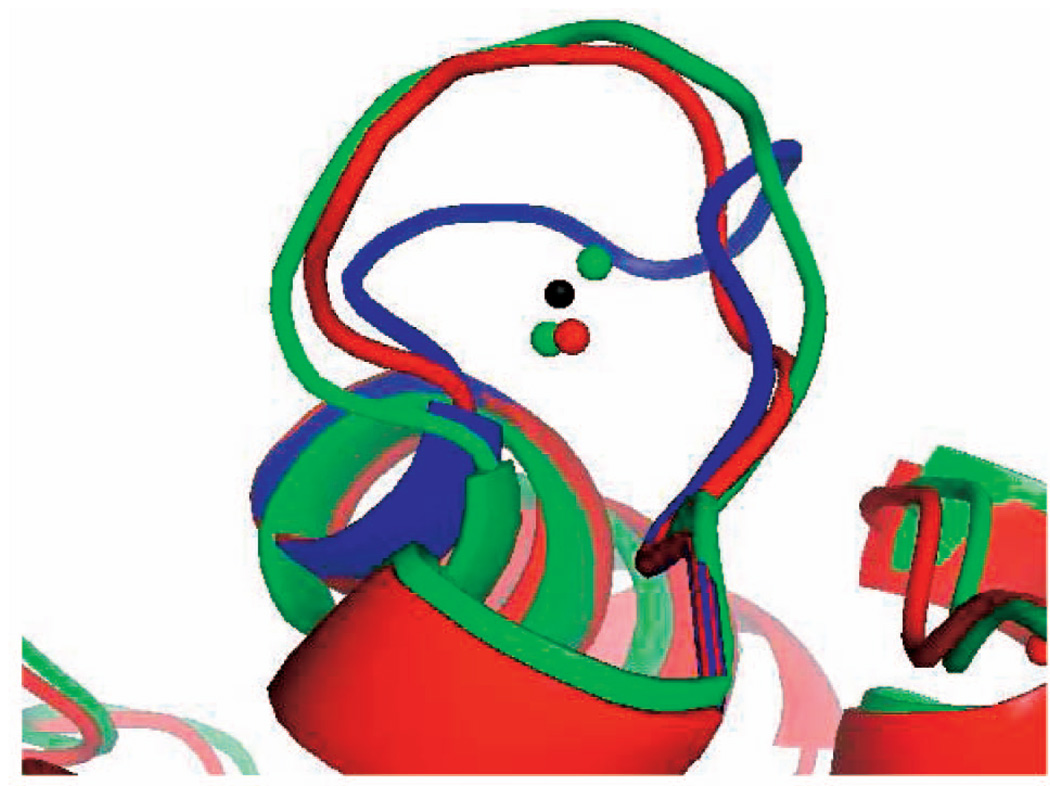
For example, Parvalbumin [7] is a calcium-binding protein, where the loop ALA51-ILE58 is a binding site that flips up upon calcium binding. The PDB codes for its apo and holo structures are 1B8C and 1B9A, respectively. In Fig. 9, these conformations are shown in blue and green, respectively; the black dot is the center of the calcium ion in the holo PDB file. We sampled successive conformations of this loop using our seed sampling procedure and ran FEATURE on each of them, until FEATURE recognized a loop conformation as a calcium-binding site. The recognized conformation, shown in red in Fig. 9, is close to the holo structure 1B9A. The red dot represents the position of the calcium ion predicted by FEATURE in this recognized conformation. Similarly, the two green dots represent positions of the calcium ion predicted by FEATURE for the green holo conformation. Note that all these dots are all very close to the calcium position recorded in the PDB. Correctly, FEATURE did not recognize the apo conformation shown in blue as a binding conformation; hence, there is no blue dot in the figure. We then explore the neighboring conformations of the seed, trying to get conformations even closer to the PDB holo state. We deformed the seed by deformation sampling until FEATURE returned a higher score than the seed. The final conformation only slightly improved the backbone RMSD to the holo conformation.

Fig. 9.

Parvalbumin loop ALA51-ILE58: The apo and holo conformations recorded in the PDB are shown in blue and green, respectively. The loop conformation in red is the conformation generated by seed sampling and recognized by FEATURE as a calcium-binding site. The black dot is the position of the calcium ion recorded in the PDB. The green and red dots are the calcium positions predicted by FEATURE for the loop conformations of the same color.

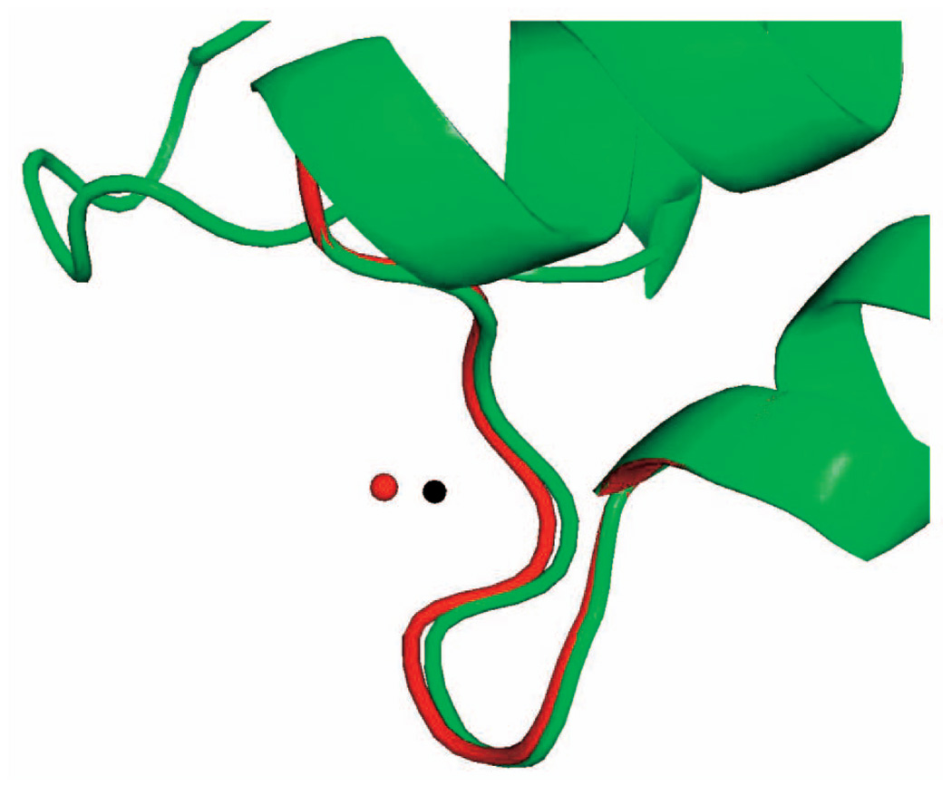
Deformation sampling can also be used to enhance the performance of FEATURE. To recognize a binding site, FEATURE counts atoms contained in concentric spherical shells. Therefore, it is somewhat sensitive to the values of the radii of the shells, as well as to the position of the center of the shells. This may cause FEATURE to fail to correctly recognize a functional state. For example, in protein grancalcin, the loop ALA62-ASP69 is a calcium-binding site [19]. The holo structure has PDB code 1K94. It is shown in green in Fig. 10, where the black dot is the position of the calcium ion recorded in the PDB. Surprisingly, FEATURE failed to recognize this structure as a binding site. So, we then used deformation sampling around the holo structure 1K94 and ran FEATURE on each one of them until FEATURE identified it as a calcium-binding site. The resulting loop conformation is shown in red in Fig. 10, where the red dot is the predicted calcium position. The main difference between the holo structure 1K94 and the conformation generated by deformation sampling is the location of ASP65, one of the four coordinating residues. Atoms from the main and side chains of ASP65 are located slightly closer to the calcium-binding site in the conformation obtained by deformation sampling. These small displacements are sufficient to change the atom counts in the spherical shells considered by FEATURE, thereby affecting the score of the entire site.

Fig. 10.

Grancalcin loop ALA62-ASP69. The holo conformation in the PDB file is shown in green. The conformation in red was generated using deformation sampling. FEATURE correctly recognized the red conformation as a calcium-binding site but failed to do so on the green conformation (see text).

7.5 Comparison with Previous Methods

Comparing methods is delicate because, as discussed in Section 2, these methods have different purposes. Thus, preferences in their solutions and evaluation metrics differ. RAPPER [12] and the hierarchical method in [18] focus on generating near-native conformations, while our methods aim at exploring the closed clash-free conformation space. The results in Section 7.4 demonstrate the ability of our methods to generate both native conformations and other biologically important conformations that significantly differ from the native ones. Such results would be difficult to obtain with the methods presented in [12] and [18].

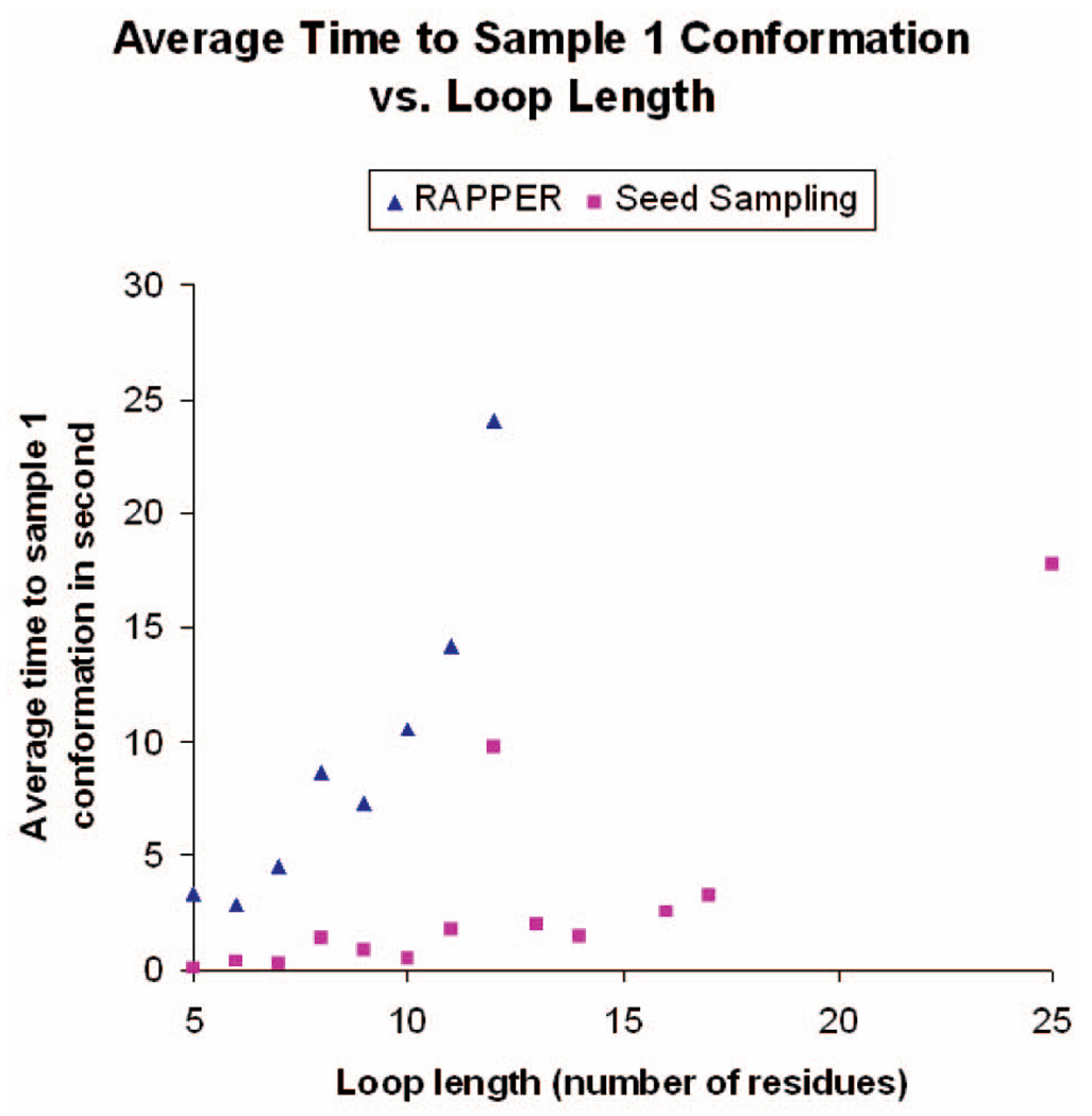
Fig. 11 plots the average running times of RAPPER (as reported in [12]) and those of our seed sampling procedure to obtain one conformation of one loop for different loop lengths. Although the absolute running times are subject to differences in computer speed and software coding, the trends shown in the figure suggest that our seed sampling method scales better than RAPPER when loop length increases. There is not enough data in [18] to provide a similar comparison.

Fig. 11.

Average running time (in seconds) to obtain one conformation by RAPPER and our seed sampling procedure for different loop lengths.

Using discrete sets of ϕ and ψ values derived from protein structure databases certainly reduces the size of the search space. In RAPPER, each residue has 5,184 states, and the method in [18] assigns 215 to 866 states to each residue. On the other hand, it may also make it more difficult to sample clash-free conformations, especially nonnative conformations. Furthermore, the methods in [12] and [18] also incur the cost of running an energy minimization algorithm to generate near-native conformations. Overall, we believe that the fact that our seed sampling procedure seems to be faster than RAPPER and to scale better with loop length is mainly due to the constraint prioritization scheme embedded in our procedure.

The paper on RLG [9] only reports tests on a single 17-residue loop (named loop 7, between Gly433 and Gly449) of protein 1G5A. The goal of the work was to study the mobility of this loop in the presence and absence of certain side chains. About 1 h was needed to generate a tree of 1,000 nodes using RLG (see Section 2), which amounts to 3.6 seconds per conformation. On this same loop, our seed sampling takes 3.28 s per conformation. However, in [9], a less stringent overlap factor was used to test atomic clashes. Moreover, it is unknown how quickly the tree generated by RLG expands across the loop’s closed clash-free conformation space. Since this tree is constructed iteratively by sampling each new conformation from an already sampled conformation, our seed sampling is likely to produce more broadly distributed conformations.

8 CONCLUSION

We have described two distinct algorithms to sample the space of closed clash-free conformations of a flexible loop. The seed sampling algorithm produces broadly distributed conformations. It is based on a novel prioritized constraint-satisfaction approach that interweaves the treatment of the clash avoidance and closure constraints. The deformation sampling algorithm uses seed conformations as starting points to explore more finely certain regions of the space. It is based on the computation of the null space of the loop backbone at its current conformation.

Early versions of these algorithms have been used successfully to interpret fuzzy regions in EDMs obtained from X-ray crystallography experiments [28]. Computational tests reported in this paper show that our algorithms can efficiently handle loops ranging from 5 to 25 residues in length. Additional tests demonstrate their ability to generate biologically interesting loop conformations, such as calcium-binding conformations. This critical ability could be used in the future to predict loop conformations and improve other structure prediction techniques, like homology, when functional information is known in advance.

Biographies

Peggy Yao received the BS degree (with first class honors) major in computer science, minor in biotechnology and the MS degree in computer science from the National University of Singapore. She is a PhD candidate in the Biomedical Informatics Department, Stanford University. Her research interests include protein 3D structure modeling, computer-aided drug design, and other areas in computational molecular biology. She is currently working on protein conformation sampling.

Ankur Dhanik received the BTech degree from the Indian Institute of Technology, Kanpur, India and the MS degree from the National University of Singapore. He is a PhD student in the Mechanical Engineering Department, Stanford University, Stanford. His research interests include computational biology, protein structure determination, protein design, and robotics.

Nathan Marz received the BS and MS degrees in computer science from Stanford University. He is currently with RapLeaf, San Francisco.

Ryan Propper received the BS degree in computer science from Stanford University in 2007. He is currently with Google. His interests include protein folding and kinematics as well as their applications in the broader studies of molecular biology and computational drug design.

Charles Kou received the BS degree in computer science from Stanford University. He is currently with the Computer Science Department, Stanford University. His interests include analyzing conformations and the motion of flexible protein loops, and homology modeling.

Guanfeng Liu received the PhD degree in electrical engineering from Hong Kong University of Science and Technology in 2003. He held visiting positions at Rensselaer Polytechnic Institute and Stanford University from 2003 to 2007. He is currently a software development engineer at Xyratex International. His research interests include robotics, automation, and manufacturing.

Henry van den Bedem received the MS degree in mathematics from Delft University of Technology, Delft, Netherlands and the PhD degree in mathematics from the University of Alabama, Birmingham. He is a staff scientist in the Joint Center for Structural Genomics (http://www.jcsg.org), Stanford Linear Accelerator Center. His interests include computational structural biology, in particular developing algorithms for interpreting structure and motion of macromolecules from experimental (crystallographic) data, and physics-based refinement of comparative protein models.

Jean-Claude Latombe received the PhD degree in computer science from the University of Grenoble, Grenoble, France, in 1977. In 1987, he joined Stanford University, where he is currently the Kumagai professor of engineering in the Computer Science Department. At Stanford, he served as the chairman of the Computer Science Department from 1997 to 2001. He has been a visiting professor at the Indian Institute of Technology (IIT) Kanpur, the Tecnolόgico de Monterrey, and the National University of Singapore. His research interests include robotics, motion planning, computational biology, surgical simulation, and graphic animation of digital characters. He is a fellow of the Association for the Advancement of Artificial Intelligence (AAAI).

Inbal Halperin-Landsberg received the BSc degree (with first class honors) major in biology and the PhD degree in genetics from Tel-Aviv University. She was a postdoctoral researcher of bioinformatics at Stanford University. She is currently with NextBio as a senior bioinformatician. Her research interests include protein 3D structure modeling, protein function prediction, and various areas in computational biology.

Russ Biagio Altman received the AB degree from Harvard College, the PhD in medical information sciences from Stanford University, and the MD degree from Stanford Medical School. He is a professor of bioengineering, genetics, and medicine (and of computer science by courtesy) and chairman of the Department of Bioengineering, Stanford University. His primary research interests are in the application of computing technology to basic molecular biological problems of relevance to medicine. He is currently developing techniques for collaborative scientific computation over the Internet, including novel user interfaces to biological data, particularly for pharmacogenomics (e.g., http://www.pharmgkb.org/). His other work focuses on the analysis of functional microenvironments within macromolecules and the application of algorithms for determining the structure, dynamics, and function of biological macromolecules (e.g., http://simbios.stanford.edu/). He was a recipient of the US Presidential Early Career Award for Scientists and Engineers, a National Science Foundation CAREER Award, and the Stanford Medical School Graduate Teaching Award in 2000. He is a past president and founding board member of the International Society for Computational Biology and an organizer of the Annual Pacific Symposium on Biocomputing. He leads one of seven NIH-supported National Centers for Biomedical Computation, focusing on physics-based simulation of biological structures (http://simbios.stanford.edu/). He is a fellow of the American College of Physicians and the American College of Medical Informatics.

References

- 1.Babor M, Greenblatt HM, Edelman M, Sobolev V. Flexibility of Metal Binding Sites in Proteins on a Database Scale. Proteins: Structure, Function, and Bioinformatics. 2005;vol. 59:221–230. doi: 10.1002/prot.20431. [DOI] [PubMed] [Google Scholar]
- 2.Bakker PIW, DePristo MA, Burke DF, Blundell TL. Ab Initio Construction of Polypeptide Fragments: Accuracy of Loop Decoy Discrimination by an All-Atom Statistical Potential and the AMBER Force Field with the Generalized Born Solvation Model. Proteins: Structure, Function, and Genetics. 2003;vol. 51:21–40. doi: 10.1002/prot.10235. [DOI] [PubMed] [Google Scholar]
- 3.Bosshard HR. Molecular Recognition by Induced Fit: How Fit Is the Concept? News in Physiological Sciences. 2001;vol. 16:171–173. doi: 10.1152/physiologyonline.2001.16.4.171. [DOI] [PubMed] [Google Scholar]
- 4.Bruccoleri RE, Karplus M. Conformational Sampling Using High Temperature Molecular Dynamics. Biopolymers. 1990;vol. 29:1847–1862. doi: 10.1002/bip.360291415. [DOI] [PubMed] [Google Scholar]
- 5.Canutescu A, Dunbrack R., Jr Cyclic Coordinate Descent: A Robotics Algorithm for Protein Loop Closure. Protein Science. 2003;vol. 12:963–972. doi: 10.1110/ps.0242703. [DOI] [PMC free article] [PubMed] [Google Scholar]
- 6.Canutescu A, Shelenkov A, Dunbrack R., Jr A Graph Theory Algorithm for Protein Side-Chain Prediction. Protein Science. 2003;vol. 12:2001–2014. doi: 10.1110/ps.03154503. [DOI] [PMC free article] [PubMed] [Google Scholar]
- 7.Cates MS, Berry MB, Ho EL, Li Q, Potter JD, Phillips GN., Jr Metal-Ion Affinity and Specificity in EF-Hand Proteins: Coordination Geometry and Domain Plasticity in Parvalbumin. Structure with Folding and Design. 1999;vol. 7:1269–1278. doi: 10.1016/s0969-2126(00)80060-x. [DOI] [PubMed] [Google Scholar]
- 8.Chang KS, Khatib O. Operational Space Dynamics: Efficient Algorithm for Modeling and Control of Branching Mechanisms. Proc. IEEE Int’l Conf. Robotics and Automation (ICRA ’00) 2000:850–856. [Google Scholar]
- 9.Cortes J, Simeon T, Renaud-Simeon M, Tran V. Geometric Algorithms for the Conformational Analysis of Long Protein Loops. J. Computational Chemistry. 2004;vol. 25:956–967. doi: 10.1002/jcc.20021. [DOI] [PubMed] [Google Scholar]
- 10.Coutsias EA, Soek C, Jacobson MP, Dill KA. A Kinematic View of Loop Closure. J. Computational Chemistry. 2004;vol. 25:510–528. doi: 10.1002/jcc.10416. [DOI] [PubMed] [Google Scholar]
- 11.Deane CM, Blundell TL. A Novel Exhaustive Search Algorithm for Predicting the Conformation of Polypeptide Segments in Proteins. Proteins: Structure, Function, and Genetics. 2000;vol. 40:135–144. [PubMed] [Google Scholar]
- 12.DePristo MA, de Bakker PIW, Lovell SC, Blundell TL. Ab Initio Construction of Polypeptide Fragments: Efficient Generation of Accurate, Representative Ensembles. Proteins: Structure, Function, and Genetics. 2003;vol. 51:41–55. doi: 10.1002/prot.10285. [DOI] [PubMed] [Google Scholar]
- 13.Fiser A, Do RKG, Sali A. Modeling of Loops in Protein Structures. Protein Science. 2000;vol. 9:1753–1773. doi: 10.1110/ps.9.9.1753. [DOI] [PMC free article] [PubMed] [Google Scholar]
- 14.Furnham N, Blundell TL, DePristo MA, Terwilliger TC. Is One Solution Good Enough? Nature Structure Molecular Biology. 2006;vol. 13:184–185. doi: 10.1038/nsmb0306-184. [DOI] [PubMed] [Google Scholar]
- 15.Glazer DS, Radmer RJ, Altman RB. Combining Molecular Dynamics and Machine Learning to Improve Protein Function Recognition. Proc. Pacific Symp. Biocomputing (PSB ’08) 2008;vol. 13:332–343. [PMC free article] [PubMed] [Google Scholar]
- 16.Golub G, van Loan C. Matrix Computations. third ed. John Hopkins Univ. Press; 1996. [Google Scholar]
- 17.Halperin D, Overmars MH. Spheres, Molecules and Hidden Surface Removal. Computational Geometry: Theory and Applications. 1998;vol. 11:83–102. [Google Scholar]
- 18.Jacobson MP, Pincus DL, Rapp CS, Day TJF, Honig B, Shaw DE, Friesner RA. A Hierarchical Approach to All-Atom Protein Loop Prediction. Proteins: Structure, Function, and Bioinformatics. 2004;vol. 55:351–367. doi: 10.1002/prot.10613. [DOI] [PubMed] [Google Scholar]
- 19.Jia J, Borregaard N, Lollike K, Cygler M. Structure of Ca2+-Loaded Human Grancalcin. Acta Crystallographica. 2001;vol. D57:1843–1849. doi: 10.1107/s0907444901016511. [DOI] [PubMed] [Google Scholar]
- 20.Kawasaki H, Kretsinger RH. Calcium-Binding Proteins 1: EF-Hands. Protein Profile. 1995;vol. 2:305–490. [PubMed] [Google Scholar]
- 21.Kolodny R, Guibas L, Levitt M, Koehl P. Inverse Kinematics in Biology: The Protein Loop Closure Problem. Int’l J. Robotics Research. 2005;vol. 24:151–163. [Google Scholar]
- 22.Levin E, Kondrashov D, Wesenberg G. Ensemble Refinement of Protein Crystal Structures: Validation and Application. Structure. 2007;vol. 15:1040–1052. doi: 10.1016/j.str.2007.06.019. [DOI] [PMC free article] [PubMed] [Google Scholar]
- 23.Okazaki K, Koga N, Takada S, Onuchic JN, Wolynes PG. Multiple-Basin Energy Landscapes for Large-Amplitude Conformational Motions of Proteins: Structure-Based Molecular Dynamics Simulations. Proc. Nat’l Academy of Sciences USA. 2006;vol. 103:11844–11849. doi: 10.1073/pnas.0604375103. [DOI] [PMC free article] [PubMed] [Google Scholar]
- 24.Sauder JM, Dunbrack R., Jr Beyond Genomic Fold Assignment: Rational Modeling of Proteins in Biological Systems. J. Molecular Biology. 2000;vol. 8:296–306. [PubMed] [Google Scholar]
- 25.Shehu A, Clementi C, Kavraki LE. Modeling Protein Conformation Ensembles: From Missing Loops to Equilibrium Fluctuations. Proteins: Structure, Function, and Bioinformatics. 2006;vol. 65:164–179. doi: 10.1002/prot.21060. [DOI] [PubMed] [Google Scholar]
- 26.Sousa SF, Fernandes PA, Ramos MJ. Protein-Ligand Docking: Current Status and Future Challenges. Proteins: Structure, Function, and Bioinformatics. 2006;vol. 65:15–26. doi: 10.1002/prot.21082. [DOI] [PubMed] [Google Scholar]
- 27.Tossato CE, Bindewald E, Hesser J, Manner R. A Divide and Conquer Approach to Fast Loop Modeling. Protein Eng. 2002;vol. 15:279–286. doi: 10.1093/protein/15.4.279. [DOI] [PubMed] [Google Scholar]
- 28.van den Bedem H, Lotan I, Latombe JC, Deacon A. Real-Space Protein-Model Completion: An Inverse-Kinematic Approach. Acta Crystallographica. 2005;vol. D61:2–13. doi: 10.1107/S0907444904025697. [DOI] [PubMed] [Google Scholar]
- 29.van Vlijmen HWT, Karplus M. PDB-Based Protein Loop Prediction: Parameters for Selection and Methods for Optimization. J. Molecular Biology. 1997;vol. 267:975–1001. doi: 10.1006/jmbi.1996.0857. [DOI] [PubMed] [Google Scholar]
- 30.Wedemeyer WJ, Scheraga HA. Exact Analytical Loop Closure in Proteins Using Polynomial Equations. J. Computational Chemistry. 1999;vol. 20:819–844. doi: 10.1002/(SICI)1096-987X(199906)20:8<819::AID-JCC8>3.0.CO;2-Y. [DOI] [PubMed] [Google Scholar]
- 31.Wei L, Altman RB. Recognizing Protein Binding Sites Using Statistical Descriptions of Their 3D Environments. Proc. Pacific Symp. Biocomputing (PSB ’98) 1998:497–508. [PubMed] [Google Scholar]