Bayesian Wombling for Spatial Point Processes

Summary

In many applications involving geographically indexed data, interest focuses on identifying regions of rapid change in the spatial surface, or the related problem of the construction or testing of boundaries separating regions with markedly different observed values of the spatial variable. This process is often referred to in the literature as boundary analysis or wombling. Recent developments in hierarchical models for point-referenced (geostatistical) and areal (lattice) data have led to corresponding statistical wombling methods, but there does not appear to be any literature on the subject in the point process case, where the locations themselves are assumed to be random and likelihood evaluation is notoriously difficult. We extend existing point-level and areal wombling tools to this case, obtaining full posterior inference for multivariate spatial random effects that, when mapped, can help suggest spatial covariates still missing from the model. In the areal case we can also construct wombled maps showing significant boundaries in the fitted intensity surface, while the point-referenced formulation permits testing the significance of a postulated boundary. In the computationally demanding point-referenced case, our algorithm combines Monte Carlo approximants to the likelihood with a predictive process step to reduce the dimension of the problem to a manageable size. We apply these techniques to an analysis of colorectal and prostate cancer data from the northern half of Minnesota, where a key substantive concern is possible similarities in their spatial patterns, and whether they are affected by each patient's distance to facilities likely to offer helpful cancer screening options.

1. Introduction

Spatially referenced data occur in diverse scientific disciplines, such as image analysis, geological and environmental sciences, ecological systems, disease mapping, and in broader public health contexts. As opposed to the usual case of measurements at fixed spatial locations, the locations themselves may be random (e.g., addresses of emerging cancer cases), in which case they should be treated as random realizations of a spatial process.

Inferential interest customarily focuses upon estimating model parameters and producing a spatial surface over the domain of interest. Once such an interpolated surface has been obtained, locating areas of rapid change on the surface may be of interest. Such local analysis of the surface (e.g., gradients at given points) has only started receiving attention. Detecting zones or boundaries of rapid change on interpolated spatial surfaces is often referred to as wombling, after a foundational article by Womble (1951). The field is also known as boundary analysis, barrier analysis, and edge detection in fields such as landscape topography, systematic biology, sociology, ecology, and image analysis. Ultimately, the underlying influences responsible for these zones or boundaries are typically of greatest scientific interest.

While boundary and cluster analysis are related, the latter detects clusters of homogeneous regions by classifying a region as a member of a particular cluster. By contrast, boundary analysis attempts to detect regions of rapid change, typically “lines” or “curves” on the spatial surface. Substantive interest focuses upon the boundary itself and what distinguishes the regions on either side, rather than on any particular region. Therefore, methods for spatial clustering (e.g., Lawson and Denison, 2002; Ma et al., 2007) are not directly applicable here. Another related problem is that of spatial extrema detection (Pascutto et al., 2000) that finds differences between locations and the state or national average. In wombling, interest instead lies in detecting sharp boundaries in the spatial relative intensity surface, so that the reasons for these rapid changes at a local scale can be investigated.

The motivating problem here involves the spatial distribution of colorectal and prostate cancers diagnosed in the state of Minnesota. These data are part of a much larger set collected by the Minnesota Cancer Surveillance System (MCSS), a program sponsored by the Minnesota Department of Health. The MCSS includes the residential address of essentially every person diagnosed with cancer in Minnesota. Here we consider the subset of men diagnosed during the period 1998−2002 (an interval chosen partly for its centering around a U.S. Census year, 2000) and residing in roughly the northern half of the state, defined here as cases with latitude greater than 45.855, the latitudinal midpoint between Minneapolis and Duluth, Minnesota. This results in 6206 cases for analysis.

Figure 1 plots the residential locations in this data, where we have added a random “jitter” to each in order to protect the confidentiality of the patients (and explaining why some of the cases appear to lie outside of the spatial domain). The research problem of interest is to detect regions of elevated colorectal or prostate cancer intensity, relative to the available population and after accounting for important spatial and nonspatial covariates. An example of the former is distance to the cancer treatment facilities (shown as triangles in Figure 1), since proximity to such sites may correlate with better screening (PSA testing, colonoscopy, etc.). We wish to identify boundaries separating zones where these residual relative intensities significantly differ. More specifically, we wish to detect regions of high gradients that often occur due to lurking spatial variables representing local disparities, such as disparities in income or access to health care. Statistically mapping such gradients can reveal “hotspots” that suggest hidden risk factors, and may also help administrators determine where to build new screening facilities, or how to expand the service regions of existing ones.

Figure 1.

Jittered residential locations of colorectal (circles) and prostate (plus signs) cancer cases, as well as major cancer treatment facilities (triangles), northern Minnesota, 1998−2002.

Estimation methods for inhomogeneous spatial point process models often avoid full likelihood evaluations by formulating estimating equations (Waagepetersen, 2007; Waagepetersen and Guan, 2008) or blocked-bootstrap algorithms (Guan and Loh, 2007). Inference on spatial associations proceeds not from the intensity surface, but from pairwise correlation functions and transforms thereof (e.g., the g and K functions described in Waagepetersen, 2007). Consequently these methods do not permit estimating gradients or wombling on the intensity surface. We instead propose a fully Bayesian approach that yields posterior distributions for the intensity surface, or even the spatial residual surface after adjusting for regressors, and for gradients (at points or along curves) and all wombling-related estimands. Inference is exact and does not rely upon possibly inappropriate use of infill or increasing-domain asymptotics.

Here we present wombling methods for estimated intensity surfaces within a hierarchical point process setting. Recently, Banerjee and Gelfand (2006) developed an inferential method for boundaries on Gaussian process surfaces, but this has been applied only to geostatistical (fixed location) models. Our current application requires modeling random locations to construct intensity surfaces. Full Bayesian inference for point process models is computationally intensive, a problem that is aggravated by a large number of spatial locations. We resort to a reduced-rank predictive process (Banerjee et al., 2008) that operates on a lower-dimensional subspace. Our contribution here is to integrate wombling methods with predictive process surfaces within a point-process framework in order to analyze the data in Figure 1.

Point process data can be converted to areal data by aggregating to regional summaries, a common data deidentification tool. Hence we compare our approach to those for areal wombling. Lu and Carlin (2005) recently developed a hierarchical statistical modeling framework to perform areal wombling. Here the underlying map and its geopolitical boundaries are considered the domain of interest. These models account for spatial association and permit borrowing of strength across the model hierarchy. Further, their Bayesian implementation enables direct estimation of the posterior probability that two geographic regions are separated by the wombled boundary.

In Section 2 we briefly review the spatial point process model and develop models for areal and point-level wombling. Section 3 then applies our models to the MCSS data, mapping boundaries of different types and testing for significance of certain pre-specified candidate boundaries. Finally, Section 4 summarizes and offers directions for future work.

2. Point Process Wombling

We provide a brief introduction to hierarchical point process modeling, referring to Liang et al. (2007) for full details. We then marry these methods to the problem of boundary analysis, taking our cues from the point-level and areal wombling literature in turn.

2.1 Point process hierarchical modeling

Consider a set of random locations $S={\left\{{\mathrm{s}}_i\right\}}_{i=1}^n$ where disease occurrence is observed over a spatial domain D. The covariates associated with each disease occurrence can be classified as spatial or non-spatial. Spatial covariates, denoted as z(s), are location-specific regardless of whether a disease occurs there or not, such as elevation, climate, exposure to pollutants, the driving distance to certain key locations, etc. Non-spatial covariates are not location-specific, but are instead case-specific, such as age, cancer stage, or education level. We further categorize some non-spatial covariates (for us, cancer type) as providing “marks,” leading to a marked point process model. Non-spatial covariates are obtainable only at locations where the disease occurs. We denote these covariates by v, and view them as “nuisance” covariates. We do not seek to distinguish point patterns by these covariates; rather, we only wish to adjust the fitted intensity surface to reflect their effects.

In general, we view the data, including locations and nuisance covariates, as a random realization from some non-homogeneous Poisson process with intensity function λ(s, v, k) defined over the product space $D\times \mathcal{V}\times \mathcal{K}$, where $\mathcal{V}$ is the nuisance covariate space and $\mathcal{K}$ is the mark space. The likelihood for the intensity surface given the data is then

$$L=\text{exp}\left(-{\int }_{D\times \mathcal{V}\times \mathcal{K}}\lambda (\mathrm{s},\mathrm{v},k)d\mathrm{s}d\mathrm{v}dk\right)\times \prod _i\lambda ({\mathrm{s}}_i,{\mathrm{v}}_i,k_i),$$ (1)

where v_i and k_i denote the non-spatial covariates and marks for the i-th case, respectively.

We let λ(s, v, k) = r(s)π(s, v, k), where r(s) is the population density surface at location s. (In practice, we may approximate this surface using areal unit population counts, setting r(s) = n(A)/|A| if s ∈ A, where n(A) is the number of points in A and |A| is the area of A.) So, r(s) serves as an offset and π(s, v, k) is interpreted as a population-adjusted (or relative) intensity. We then set π(s, v, k) = exp{β_0k + z(s)^Tβ_k + v^Tα_k + w_k(s)}, where w_k(s) is a zero-centered stochastic process, and β_0k, β_k and α_k are unknown regression coefficients. With w(s) a Gaussian process and no non-spatial covariates, the original point process becomes a log Gaussian Cox process (LGCP; Møller and Waagepetersen, 2004, p.72).

A key advantage in the likelihood computation emerges from the additive form in z(s) and v. Let {(s_ki, v_ki), i = 1, 2,...n_k} be the locations and nuisance covariates associated with the n_k points having mark k. The likelihood (1) becomes

$$\prod _k\text{exp}\left(-{\int }_D{\int }_{\mathcal{V}}\lambda (\mathrm{s},\mathrm{v},k)d\mathrm{v}d\mathrm{s}\right)\times \prod _k\prod _{{\mathrm{s}}_{ki},{\mathrm{v}}_{ki}}\lambda ({\mathrm{s}}_{ki},{\mathrm{v}}_{ki}).$$ (2)

Inserting the expression for π(s, v, k) in (2), we obtain

$$\begin{array}{cc}\hfill & \prod _k\text{exp}\left(-q({\beta }_{0k},{\alpha }_k){\int }_{D}r\left(\mathrm{s}\right)\text{exp}\{{\mathrm{z}}^T\left(\mathrm{s}\right){\beta }_k+w_k\left(\mathrm{s}\right)\}ds\right)\hfill \\ \hfill & \times \prod _k\prod _{i=1}^{n_k}\left[\text{exp}({\beta }_{0k}+{\mathrm{v}}_{ki}^T{\alpha }_k)r\left({\mathrm{s}}_{ki}\right)\text{exp}\{{\mathrm{z}}^T\left({\mathrm{s}}_{ki}\right){\beta }_k+w_k\left({\mathrm{s}}_{ki}\right)\}\right],\hfill \end{array}$$ (3)

where $q({\beta }_{0k},{\alpha }_k)={\int }_{\mathcal{V}}\text{exp}({\beta }_{0k}+{\mathrm{v}}^T{\alpha }_k)d\mathrm{v}$ can be evaluated analytically and the only numerical integration required is over D in the likelihood. This is still challenging as the intensity function involves the stochastic process w_k(s) thereby precluding a closed form. Berman and Turner (1992) and Hossain and Lawson (2008) explore direct evaluation of point process likelihoods using numerical quadrature. We instead opt for a Monte Carlo approximation: for a uniformly drawn random set of locations in D, say $\mathcal{C}=\{{\mathrm{t}}_j,j=1,2,\cdots ,J\}$, we write

$${\int }_{D}r\left(\mathrm{s}\right)\text{exp}\{{\mathrm{z}}^T\left(\mathrm{s}\right){\beta }_k+w_k\left(\mathrm{s}\right)\}d\mathrm{s}\approx {\mathcal{F}}_k({\mathrm{t}}_1,{\mathrm{t}}_2,\cdots ,{\mathrm{t}}_J),$$ (4)

where ${\mathcal{F}}_k({\mathrm{t}}_1,{\mathrm{t}}_2,\cdots ,{\mathrm{t}}_J)=(\mid D\mid ∕J){\Sigma }_{j}r\left({\mathrm{t}}_j\right)\text{exp}\{{\mathrm{z}}^T\left({\mathrm{t}}_j\right){\beta }_k+w_k\left({\mathrm{t}}_j\right)\}$ is the Monte Carlo sum (Møller and Waagepetersen, 2004). Plugging (4) into (3) yields the likelihood approximation

$$\prod _k\text{exp}\{-q({\beta }_{0k},{\alpha }_k){\mathcal{F}}_k({\mathrm{t}}_1,\cdots ,{\mathrm{t}}_J)\}\prod _{i=1}^{n_k}\text{exp}({\beta }_{0k}+{\mathrm{v}}_{ki}^T{\alpha }_k)r\left({\mathrm{s}}_{ki}\right)\text{exp}\{{\mathrm{z}}^T\left({\mathrm{s}}_{ki}\right){\beta }_k+w_k\left({\mathrm{s}}_{ki}\right)\}.$$ (5)

The additive form in z(s) and v imposes a “separable” or multiplicative effect of v on the spatial intensity. Including interaction terms in π(s, v, k) yields

$$\pi (\mathrm{s},\mathrm{v},k)=\text{exp}\{{\beta }_{0k}+{\mathrm{z}}^T\left(\mathrm{s}\right){\beta }_k+{\mathrm{v}}^T{\alpha }_k+{(\mathrm{v}\otimes \mathrm{z}\left(\mathrm{s}\right))}^T{\gamma }_k+w_k\left(\mathrm{s}\right)\}.$$ (6)

Here $\mathrm{v}\otimes \mathrm{z}\left(\mathrm{s}\right)$ denotes the set of all the first order interaction terms between z(s) and v. The corresponding coefficient in γ_k is set to zero when a given interaction term is excluded. With v categorical, the integral in (2) is no more difficult than in the additive case, while with v continuous, we get that ${\int }_D{\int }_{\mathcal{V}}\lambda (\mathrm{s},\mathrm{v},k)dvds$ is equal to

$${\int }_D\left(r\left(\mathrm{s}\right)\text{exp}({\beta }_{0k}+\mathrm{z}{\left(\mathrm{s}\right)}^T{\beta }_k+w_k\left(\mathrm{s}\right)){\int }_{\mathcal{V}}\text{exp}({\mathrm{v}}^T{\alpha }_k+{(\mathrm{v}\otimes \mathrm{z}\left(\mathrm{s}\right))}^T{\gamma }_k)d\mathrm{v}\right)d\mathrm{s}.$$

The innermost integral is available analytically, and the integration with respect to s can then be done as in (4). The specifications of w_k(s) may depend upon the data and the researcher's interest. The next two subsections present two model specifications that lead to what we term point process areal and point-level wombling, respectively.

2.2 Point process areal wombling

Confidentiality rules often compel researchers to aggregate point-referenced locations to areal regions (e.g., census tracts). In this case, we set w_k(s) = w_ki if s ∈ region i, whence the spatial residual surface is a tiled surface. Conditionally autoregressive (CAR) models (Besag, 1974) or their multivariate (MCAR) versions (Mardia, 1988) that use the Markovian dependence on the adjacency structure become natural models for the {w_ki}.

Since the spatial residuals are now regional characteristics, wombling on the spatial residual surface reveals boundaries between unmeasured spatially varying covariates that affect the regional intensity surface. Following Lu and Carlin (2005), we may define the boundary likelihood value (BLV) for mark k as Δ_ij,k = |w_ki – w_kj| for any two adjacent regions i and j. Crisp and fuzzy wombling boundaries are then based upon the posterior distributions of these BLVs. In the crisp case, we can define the edge between region i and j as part of the boundary if E(Δ_ij,k|Data) > c for some constant c > 0, or if P(Δ_ij,k > c|Data) > c* for some constant 0 < c* < 1. In the fuzzy case, resulting maps have their edges shaded according to the P(Δ_ij,k > c|Data) themselves, to reflect the relative probabilities of being part of the boundary. MCMC samples of the model parameters can be obtained through standard (e.g., Metropolis-Hastings) algorithms, hence we can readily obtain posterior samples ${\Delta }_{ij,k}^{\left(g\right)},g=1,2,\cdots ,G$. Then $\widehat{E}({\Delta }_{ij,k}\mid Data)=\frac{1}{G}{\sum }_g{\Delta }_{ij,k}^{\left(g\right)}$, and $\widehat{P}({\Delta }_{ij,k}>c\mid Data)=\frac{\#{\Delta }_{ij,k}^{\left(g\right)}>c}{G}$.

We can also womble on the (log) relative intensity surface itself, in order to find boundaries separating regions of significantly different fitted intensity. The BLV between any two adjacent regions i and j might be taken to be the absolute difference between the values of the intensity function at the corresponding centroids c_i and c_j at some typical non-spatial covariate values v₀, namely, ${\Delta }_{ij,k}=\mid \pi ({\mathrm{c}}_i,{\mathrm{v}}_0,k)-\pi ({\mathrm{c}}_j,{\mathrm{v}}_0,k)\mid$. An alternate definition is ${\Delta }_{ij,k}=\mid {\int }_{D_i}\pi (\mathrm{s},{\mathrm{v}}_0,k)d\mathrm{s}-{\int }_{D_j}\pi (\mathrm{s},{\mathrm{v}}_0,k)d\mathrm{s}\mid$, which can be interpreted as the absolute difference in the aggregate occurrence rates.

Finally, we remark that the model in this subsection reduces to the multivariate extension of Lu and Carlin (2005) in the case where all spatial covariates are observed at areal level. This is not the case in our MCSS data, however, as distance to nearest screening and radiation treatment facility is a spatially continuous covariate.

2.3 Point process point-referenced wombling

2.3.1 Curvilinear wombling

Banerjee and Gelfand (2006) propose a Bayesian point-level wombling framework for any mean-squared differentiable surface Y(s), which can be either the spatial residual surface or the log relative intensity surface. For any open curve C, the wombling measure of the curve is defined as the total or the average gradient along C, ${\int }_C{D}_{n\left(\mathrm{s}\right)}Y\left(\mathrm{s}\right)dv={\int }_C\langle \nabla Y\left(\mathrm{s}\right),n\left(\mathrm{s}\right)\rangle dv$ and $\frac{1}{v\left(C\right)}{\int }_C{D}_{n\left(\mathrm{s}\right)}Y\left(\mathrm{s}\right)dv=\frac{1}{v\left(C\right)}{\int }_C\langle \nabla Y\left(\mathrm{s}\right),n\left(\mathrm{s}\right)\rangle dv$, respectively, where $\langle \cdot ,\cdot \rangle$ is the Euclidean inner product, n(s) is the normal direction to C, D_n(s)Y(s) is the directional derivative along n(s), and ν(C) is the arc length of C. For a closed curve C, these measures are related to the concept of “flux” of the region bounded by C. Banerjee and Gelfand (2006) derive the distribution theory for the above wombling measures, and propose to determine whether a curve is a “boundary curve” or not based on the posterior distribution (e.g, declaring a boundary if the 95% posterior probability interval for the wombling measure excludes zero). In practice, the curve C consists of a sequence of linear segments, and the posterior distributions of the wombling measures associated with each linear segment are obtained. The wombling measure for the entire curve is then a weighted sum, with the lengths of the comprising line segments as the weights.

2.3.2 Predictive point-process models

Another challenge presented by our MCSS data is the large number of locations n, which precludes direct computation of Gaussian process models that involve inversion of the (n + J) × (n + J) covariance matrix, where J is the number of points used to approximate the integral. To tackle this problem, we adopt a process-based “reduced-rank kriging” approach (Banerjee et al., 2008) that replaces the original process with a dimension-reducing predictive process model residing on a lower-dimensional subspace generated by a smaller number of sites, or knots. With K marks, assume w(s) = (w₁(s), . . . , w_K(s))^T to be a multivariate Gaussian process, MVGP(0, Γ_w(·, ·; θ)), where ${\Gamma }_{\mathrm{w}}(\mathrm{s},{\mathrm{s}}^{\prime };\theta )={\left[Cov(w_i\left(\mathrm{s}\right),w_j\left({\mathrm{s}}^{\prime }\right))\right]}_{i,j=1}^K$ is the K × K cross-covariance matrix function. The predictive process corresponding to this multivariate process is the predictor of w(s) based upon the realizations ${\mathrm{w}}^{\ast }={(\mathrm{w}{\left({\mathrm{s}}_1^{\ast }\right)}^T,\dots ,\mathrm{w}{\left({\mathrm{s}}_m^{\ast }\right)}^T)}^T$ of w(s) over a collection of m sites $S^{\ast }=\{{\mathrm{s}}_1^{\ast },\dots ,{\mathrm{s}}_m^{\ast }\}$, where m is much smaller than n. Given S*, the predictive process is the spatial interpolator $\tilde{\mathrm{w}}\left(\mathrm{s}\right)=E[\mathrm{w}\left(\mathrm{s}\right)\mid {\mathrm{w}}^{\ast }]=r^T(\mathrm{s};\theta ){\Gamma }^{\ast }\left(\theta \right){\mathrm{w}}^{\ast }$, where $r^T(\mathrm{s};\theta )={\left[{\Gamma }_{\mathrm{w}}(\mathrm{s},{\mathrm{s}}_j^{\ast };\theta )\right]}_{j=1}^m$ is the K × mK cross-covariance matrix. We call $\tilde{\mathrm{w}}\left(\mathrm{s}\right)$ the predictive process derived from the parent process w(s). Computational gains accrue from w* ∼ MV N(0, Γ*(θ)) where ${\Gamma }^{\ast }\left(\theta \right)={\left[{\Gamma }_{\mathrm{w}}({\mathrm{s}}_i^{\ast },{\mathrm{s}}_j^{\ast };\theta )\right]}_{i,j=1}^m$ is a mK × mK dispersion matrix, instead of the much larger nK × nK matrices corresponding to w. Replacing w(s) in (5) with $\tilde{\mathrm{w}}\left(\mathrm{s}\right)$ we obtain

$$\prod _k\text{exp}\left\{-q({\beta }_{0k},{\alpha }_k){\tilde{\mathcal{F}}}_k({\mathrm{t}}_1,\cdots ,{\mathrm{t}}_J)\right\}\prod _{i=1}^{n_k}\text{exp}({\beta }_{0k}+{\mathrm{v}}_{ki}{\alpha }_k)r\left({\mathrm{s}}_{ki}\right)\text{exp}\{{\mathrm{z}}^T\left({\mathrm{s}}_{ki}\right){\beta }_k+{\tilde{w}}_k\left({\mathrm{s}}_{ki}\right)\},$$ (7)

where $\tilde{\mathcal{F}}$ is obtained by replacing each w_k(t_j) in $\mathcal{F}$ with ${\tilde{w}}_k\left({\mathrm{t}}_j\right)=r_k^T({\mathrm{t}}_j;\theta ){\Gamma }^{\ast }\left(\theta \right){\mathrm{w}}^{\ast }$ where $r_k^T(\mathrm{t};\theta )$ is the k-th row of r^T(t; θ). The predictive process inherits the attractive properties of the conditional expectation as an orthogonal projection and offers an optimal approximation to the original likelihood within a Kullback-Leibler paradigm.

We conclude with some remarks on knot selection. With evenly distributed of data locations, one possibility is to select knots on a uniform grid overlaid on the domain. Selection can then be achieved through a formal design-based approach that minimizes a spatially averaged predictive variance criterion (see, e.g., Diggle and Lophaven, 2006). However, in general the locations are highly irregular, generating substantial areas of sparse observations where we wish to avoid placing knots, since they would be “wasted” and possibly lead to inflated predictive process variances and slower convergence. Here we implement the space-covering design algorithms (e.g., Royle and Nychka, 1998) that yield a representative collection of knots that better cover the domain. Other alternatives include popular clustering algorithms such as k-means or more robust median-based partitioning around medoids algorithms (e.g., Kaufmann and Roseauw, 1990). User-friendly implementations of these algorithms are available in R packages such as fields and cluster.

2.3.3 Gradients on predictive process surfaces

We assume a stationary and separable cross-covariance function ${\Gamma }_{\mathrm{w}}(\mathrm{s},{\mathrm{s}}^{\prime };\theta )=\rho (\mathrm{s},{\mathrm{s}}^{\prime };\theta )\Sigma$, where ρ(s, s′; θ) is a stationary univariate correlation function and Σ is a K × K covariance matrix (see Subsection 3.2). Thus, Γ_w(s, s′; θ) inherits its smoothness properties from ρ(s, s′; θ), which we assume is infinitely differentiable whenever ||s–s′|| > 0. Since the elements of r^T (s; θ) share the same smoothness as ρ(s, s′; θ), $\tilde{\mathrm{w}}\left(\mathrm{s}\right)$ is infinitely differentiable (almost surely) everywhere in the domain, except possibly for $\mathrm{s}\in {\mathcal{S}}^{\ast }$. Mean square differentiability is also immediate since w* is Gaussian with a finite variance. Consequently, for cross-covariances built from, say, the Matérn correlation family, even with ν < 1 (e.g., with the exponential correlation function) so that the parent process w(s) is not mean square differentiable, the predictive process still is.

For posterior inference, we first form the finite difference directional predictive process with respect to a fixed direction (say, the unit vector u) as ${\tilde{\mathrm{w}}}_{h,\mathrm{u}}\left(\mathrm{s}\right)=\{\tilde{\mathrm{w}}(\mathrm{s}+h\mathrm{u})-\tilde{\mathrm{w}}\left(\mathrm{s}\right)\}∕h$. Being a linear function of two Gaussian processes, $\tilde{\mathrm{w}}(\mathrm{s}+h\mathrm{u})$ and $\tilde{\mathrm{w}}\left(\mathrm{s}\right),{\tilde{\mathrm{w}}}_h\left(\mathrm{s}\right)$ is itself a Gaussian process. Using a limiting argument for Gaussian processes, we have

$$\underset{h\to 0}{\lim }{\tilde{w}}_{h,\mathrm{u}}\left(\mathrm{s}\right)=\underset{h\to 0}{\lim }\frac{r^T(\mathrm{s}+h\mathrm{u};\theta )-r^T(\mathrm{s};\theta )}{h}{\Gamma }^{\ast -1}\left(\theta \right){\mathrm{w}}^{\ast }=D_{\mathrm{u}}{r}^T(\mathrm{s};\theta ){\Gamma }^{\ast -1}\left(\theta \right){\mathrm{w}}^{\ast }.$$ (8)

Since w* ∼ MV N(0, Γ*(θ)), (8) implies that $D_{\mathrm{u}}\tilde{\mathrm{w}}\left(\mathrm{s}\right)={\text{lim}}_{h\to 0}{\tilde{w}}_{h,\mathrm{u}}\left(\mathrm{s}\right)$ is a non-stationary Gaussian process $GP(0,{\tilde{\rho }}_{\mathrm{u}}(\cdot ))$, where ${\tilde{\rho }}_{\mathrm{u}}(\mathrm{s},{\mathrm{s}}^{\prime })=D_{\mathrm{u}}{r}^T(\mathrm{s};\theta ){\Gamma }^{\ast -1}\left(\theta \right)D_{\mathrm{u}}r({\mathrm{s}}^{\prime };\theta )$. More generally, for K marks, we compute the 2 × K gradient matrix $\nabla \tilde{\mathrm{w}}\left(\mathrm{s}\right)={[\partial {\tilde{w}}_j\left(\mathrm{s}\right)∕\partial s_i]}_{i=1,2}^{j=1,\cdots ,K}$. Stacking up the elements of this matrix into a 2K × 1 column vector, we find that this vector will follow a multivariate Gaussian process $MVGP(0,{\Gamma }_{\nabla }^T(\mathrm{s};\theta ){\Gamma }^{\ast -1}\left(\theta \right){\Gamma }_{\nabla }({\mathrm{s}}^{\prime };\theta ))$, where ${\Gamma }_{\nabla }^T(\mathrm{s};\theta ){\Gamma }^{\ast -1}\left(\theta \right){\Gamma }_{\nabla }({\mathrm{s}}^{\prime };\theta )$ is the 2K × 2K cross-covariance matrix with ${\Gamma }_{\nabla }^T(\mathrm{s};\theta )$ denoting the 2K × mK matrix obtained by applying ∇ to each of the components of r^T(s; θ). Posterior inference is straightforward in a sampling-based framework: having obtained the posterior samples ${\{{\mathrm{w}}^{\ast \left(l\right)},{\theta }^{\left(l\right)}\}}_{l=1}^L$, posterior samples of the predictive process gradient are obtained by setting $\nabla {\tilde{\mathrm{w}}}^{\left(l\right)}\left({\mathrm{s}}_0\right)={\Gamma }_{\nabla }^T({\mathrm{s}}_0;{\theta }^{\left(l\right)}){\Gamma }^{\ast -1}\left({\theta }^{\left(l\right)}\right){\mathrm{w}}^{\ast \left(l\right)}$ for l = 1, . . . , L.

3. Application to the Colorectal and Prostate Cancer Data

We now turn to the analysis of the MCSS colorectal and prostate cancer data using the methods of Sections 2.2 and 2.3. We consider two location-specific covariates: z₁(s), the log standardized distance to the nearest cancer treatment site (as indicated by the presence of a licensed radiation treatment facility), and z₂(s), the poverty rate in the census tract containing s. We also employ two non-location-specific covariates: v₁, cancer stage, set to 1 if the cancer is diagnosed late (regional or distant stage) and 0 otherwise, and v₂, the patient's age at diagnosis. The population density r(s) we use for standardization is available at 2000 census tract level, meaning that we assume population density is constant across any tract.

The first and second rows of Figure 2 show maps of the raw median non-spatially varying covariates (age and proportion diagnosed late), while the third row maps a crude estimate of the log-relative intensities for the colorectal (left column) and prostate (right column) cancer cases. These summaries are presented at tract level, even though we have exact (or nearly exact) spatial coordinates here. In the first two rows, tracts containing no participants are simply shaded according to the overall observed median values, which are approximately 0.1 for (centered) age for both cancers, and 0.513 and 0.161 for proportion diagnosed late in the colorectal cancer and prostate cancer groups, respectively. None of these four maps show strong spatial patterns, though we do see several rural areas with higher or lower than average age, late diagnosis fraction, or both. The third row maps the logs of the numbers of patients divided by total number of residents in each tract. This crude estimate of the tract-level log-relative intensity (unadjusted for any spatial or nonspatial covariates) indicates a fairly “flat” map, except for a few northwestern census tracts without any colorectal cancers.

Figure 2.

Minnesota cancer covariate and response data for the colorectal (left column) and prostate (right column) cases: top row, tract-specific map of observed median age; middle row, tract-specific map of observed proportion of late diagnosis; bottom row, tract-specific observed log-relative intensity (count divided by population).

Figure 3 shows tract-level maps of population density, r(s), and our two location-specific covariates, z₁(s) and z₂(s). Again we give a tract-level display here, but emphasize that z₁(s) is actually available for all s. Population density is fairly uniform over all but the most urban tracts, and z₁(s) (distance to nearest treatment site) appears exactly as expected. In the poverty map, the large and dark-shaded north-central tract that looks like a letter “P” rotated 90 degrees clockwise is the Red Lake Indian Reservation.

Figure 3.

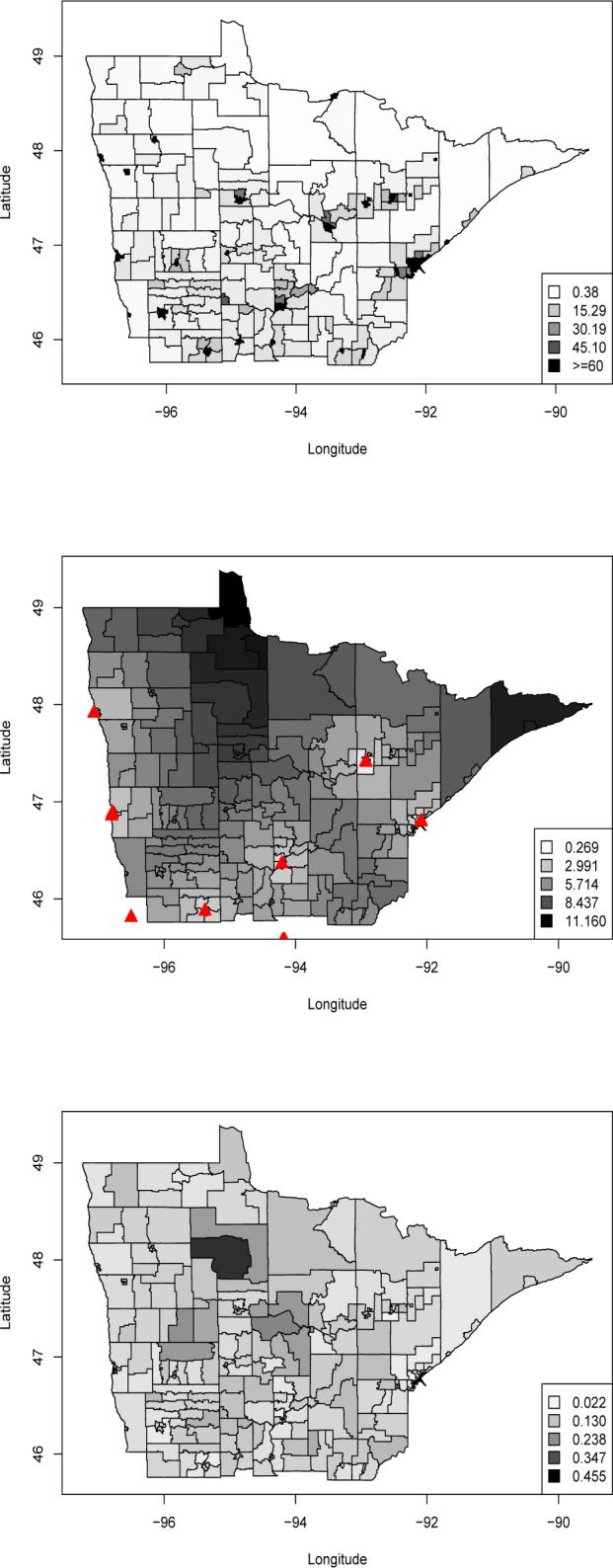
Top, population density per square kilometer by tract; middle, log-standardized distance to nearest treatment site by tract; bottom, poverty rate by tract.

We use Monte Carlo integration to approximate the integral of the intensity in (4). To do this, within each of the n_D = 261 census tracts D_i, we randomly generate n_i points {t_ij, j = 1, · · · , n_i}. The integrated intensity surface is then given by ${\int }_{\cup D_i}\lambda \left(\mathrm{s}\right)={\Sigma }_{i=1}^{n_D}{\int }_{D_i}\lambda \left(\mathrm{s}\right)d\mathrm{s}$, where the integrated intensity over each stratum is approximated by the Monte Carlo sum for the predictive process likelihood as described in (4). We compare three strategies for choosing t_ij's: the first draws points uniformly distributed over the spatial domain, the second maintains roughly the same number of points within each census tract, and the third samples proportionally to tract area and also accounts for its population density (thus, for small areas that are densely populated, we add more points). We use 2000 different posterior β samples to compute the integral, and compare the results in each case to a “benchmark” integral evaluated using using 261,000 points with about 1000 points in each census tract. We checked the median absolute differences (and their 2.5% and 97.5% percentiles) using these three strategies using roughly 10, 50, and 100 points per tract. The benchmark integral evaluates to approximately 6206 (the total number of observations), but varies between 5951 and 6492 over the 2000 β samples. With 100 points per census tract, we find that all three methods offer satisfactory approximations to the benchmark, with the relative error across the 2000 samples never being more than than 0.08%.

The population varies moderately across census tracts (from 856 to 8916) but their areas vary significantly, implying substantial variability in population density (from 0.3846/km² to 3767.0/km²) over the northern Minnesota census tracts. Our integrand, therefore, lacks smoothness, complicating its numerical evaluation. For subsequent inference we adopt the second strategy for choosing the t_ij's, using approximately 100 randomly selected points within each of our 261 census tracts, resulting in 26,100 points.

3.1 Areal wombling

As described in Section 2.2, in this case the spatial residual surface is a tiled surface. We assume that $p\left(\mathrm{w}\right)\propto \text{exp}\left\{-\frac{{\mathrm{w}}^T{\Sigma }^{-1}\otimes (D_w-W)\mathrm{w}}{2}\right\}$, i.e. the spatial residuals w follow an MCAR distribution, where $\Sigma =\left(\begin{array}{cc}\hfill {\sigma }_1^2\hfill & \hfill \rho {\sigma }_1{\sigma }_2\hfill \\ \hfill \rho {\sigma }_1{\sigma }_2\hfill & \hfill {\sigma }_2^2\hfill \end{array}\right)$, ${\sigma }_1^2$ and ${\sigma }_2^2$ are within-cancer spatial variance parameters, and ρ ∈ (−1, 1) represents the correlation between colorectal and prostate cancer. We use this model to perform boundary analysis on both the spatial residual surface and the log relative intensity surface for our MCSS dataset.

We apply our areal wombling models to the spatial residuals using a cut-off value c = log(1.5). Thus, conditioning on all the other factors, we regard tracts as meaningfully different if their relative intensities differ by 50%. We consider edges that have P(Δ_ij > c|Data) > 0.8 to be crisp wombling boundaries. The top row of Figure 4 shows wombling boundaries for the spatial residual surface. Boundaries are shown as thick white lines between the regions, which are themselves shaded according to their fitted w_ki. The left panel shows the wombled residual boundaries for colorectal cancers, while the right panel corresponds to prostate cancers. The patterns for colorectal and prostate cancers are very similar – almost identical. A few northwestern census tracts are isolated from their neighbors due to their low fitted relative intensities (hence the need for fairly large negative residuals here). Overall, there is some evidence of separation of the northern and southern parts of the map, perhaps indicating the need for more aggressive screening for both cancers in the former.

Figure 4.

Areal wombling boundaries (thick white lines), MCSS colorectal and prostate cancer data. Left panels, colorectal cancer; right panels, prostate cancer. Top row, spatial residual surface; bottom row, fitted log intensity surface. The five arrows indicate candidate areal wombling boundaries to be tested for significance in the text.

The upper left panel of Figure 4 shows the Red Lake Indian Reservation tract to be almost entirely isolated from its neighbors for colorectal cancer, which is consistent with the raw data in the lower left corner of Figure 2. To investigate this issue more carefully, we calculated the sample posterior probability that all five of the Δ_ij corresponding to the five boundary segments that form the Red Lake tract's perimeter were greater than log(1.5). We obtained probability estimates of 0.63 and 0.29 for colorectal and prostate cancer, respectively, consistent with the appearance of the top row of Figure 4.

Next, we apply this same method to the estimated log intensity surfaces which depend upon the non-spatial covariates (age and stage at diagnosis). Hence we womble on the log intensity surface for a patient of mean age who received an early diagnosis. Defining π_i,k to be the log intensity value at the centroid of region i for treatment k at the specified age and diagnosis stage, the corresponding BLV's are then Δ_ij,k = |π_i,k – π_j,k|. The bottom row of Figure 4 shows the resulting wombled boundaries, again using c = log(1.5). Our method again successfully isolates the two rural, low-density census tracts in the northwest, suggesting that these census tracts have very different cancer relative intensities from their neighbors on both the fitted and residual scales.

3.2 Point-level wombling

The point wombling methods discussed in Subsection 2.3 require the target function to be mean-square differentiable. The presence of discontinuous covariates precludes such point wombling analysis on the fitted log intensity surface, but our spatial residual surfaces remain mean-square differentiable and permit inference on gradient processes. We assume that w(s) = (w₁(s), w₂(s))^T is a bivariate Gaussian process GP(0, Γ_w(·, ·, θ)) with ${\Gamma }_{\mathrm{w}}(\cdot ,\cdot ,\theta )=\Lambda \otimes \varrho (\cdot ,\varphi )$, where $\Lambda =\left(\begin{array}{cc}\hfill {\sigma }_1^2\hfill & \hfill \rho {\sigma }_1{\sigma }_2\hfill \\ \hfill \rho {\sigma }_1{\sigma }_2\hfill & \hfill {\sigma }_2^2\hfill \end{array}\right)$ and $\varrho (\cdot ,\varphi )$ is the univariate exponential correlation function. The scale of the spatial decay parameter ϕ depends on the distance function employed. To ensure the positive definiteness of the resulting covariance matrix, we project longitude and latitude onto planar coordinates using an azimuthal projection (preserving distance from each point to the north pole), enabling us to use Euclidean distance. As is often the case, the spatial range parameter ϕ is only weakly identified (i.e., identifiable, but difficult to estimate), so an informative prior is needed for satisfactory MCMC behavior. For simplicity, we might simply fix this parameter at a value that specifies an effective spatial range equal to some fraction f (1/2, 1/4, 1/8, etc.) of the maximal inter-site distance. After experimenting with various values of f, we selected f = 1/2, or ϕ = 66, as it seemed to provide the best model fit as well as sensible fitted surfaces.

Table 1 displays estimates from our predictive process model with different numbers of knots, and from a simple areally aggregated Poisson regression model. The spatial coefficients are initially sensitive to the choice of knots, but stabilize with more than 200 knots. The non-spatial coefficients (age and late) are very robust. We also notice that the distance effect is significantly negative in the point process model, while it is not identified as significant by the Poisson model. This might be because the distance from a tract centroid to the nearest treatment facility is not that representative for many rural cases. Our model indicates relative risk tends to be lower in rural areas than in urban areas. The Poisson regression model fails to identify age as a significant risk factor for either cancer, and even leans slightly negative for prostate cancer, in strong conflict with intuition and past research. This is apparently the result of ecological fallacy: the aggregate Poisson model is forced to use average age as a predictor, and this is not an effective strategy. In contrast, our predictive point process models correctly identify a significant positive effect of age on the relative intensities of both cancers. These estimates agree extremely well over a range of between 26,100 and 52,000 t_ij's using 200 knots. Finally, the correlation parameter ρ is estimated to be about 0.95, much higher than that from the Poisson model (0.76), indicating that the residuals for these two groups have very similar patterns. In summary, Table 1 indicates that aggregation brings about a loss of accuracy of the point estimates, and of their statistical significance as well.

Table 1.

Sensitivity of parameter estimates for the Bayesian point process model with different number of knots. Results for the areal Poisson model are also shown for comparison; in this aggregate data model, “distance” is the distance from the centroid of the census tract to nearest treatment facility, “age” is the mean observed age, and “late” is the proportion of late diagonosed patients within each census tract.

	Point Process Models			Poisson Model
	64 knots	200 knots	256 knots	(areal)
colorectal:
intercept	−8.65 (−8.87,−8.48)	−7.97 (−8.17,−7.72)	−8.02 (−8.12,−7.77)	−6.30 (−6.58,−6.02)
distance	−0.04 (−0.07,−0.01)	−0.17 (−0.20,−0.14)	−0.16 (−0.19,−0.13)	0.03 (−0.01,0.07)
poverty	−0.97 (−1.83,−0.22)	−1.06 (−1.84,−0.25)	−1.09 (−1.81,−0.31)	−0.99 (−1.93,−0.06)
age	0.25 (0.23,0.27)	0.25 (0.23,0.27)	0.25 (0.23,0.27)	0.06 (−0.04,0.16)
late	0.05 (−0.04,0.14)	0.05 (−0.04,0.14)	0.06 (−0.03,0.14)	−0.05 (−0.32,0.21)
prostate:
intercept	−6.40 (−6.62,−6.29)	−5.76 (−5.89,−5.62)	−5.80 (−6.03,−5.58)	−5.06 (−5.24,−4.84)
distance	−0.11 (−0.13,−0.08)	−0.25 (−0.27,−0.24)	−0.23 (−0.26,−0.20)	0.01 (−0.02,0.04)
poverty	−2.97 (−3.59,−2.38)	−3.32 (−3.97,−2.63)	−3.25 (−4.01,−2.71)	−2.85 (−3.55,−2.15)
age	0.25 (0.24,0.27)	0.26 (0.24,0.27)	0.25 (0.24,0.27)	−0.03 (−0.17,0.11)
late	−1.65 (−1.73,−1.58)	−1.65 (−1.73,−1.58)	−1.65 (−1.72,−1.59)	−0.08 (−0.45,0.29)
ρ	0.93 (0.90,0.97)	0.95 (0.91,0.99)	0.96 (0.90,0.99)	0.76 (0.59,0.87)
${\sigma }_1^2$	0.62 (0.44,0.89)	2.91 (2.34,3.57)	2.95 (2.25,3.70)	0.71 (0.52.0.96)
${\sigma }_2^2$	1.46 (1.02,2.07)	4.05 (3.19,4.97)	3.92 (2.15,4.88)	0.82 (0.49,1.21)

Turning to mapped summaries, the top panels of Figure 5 show image-contour maps of the estimated spatial residuals under the point process model. We see a few similarities with the areally-wombled spatial residual maps in the top row of Figure 4, but overall the spatial pattern is not very strong, and we see only a few patches with high residuals. However, because the underlying spatial surface is now assumed to be continuous, we are able to see finer scale changes in the fitted surface (subject of course to the image plot's resolution).

Figure 5.

Image-contour maps of estimated spatial residuals (top row) and mean predicted gradient surfaces (bottom row), point-level wombling on MCSS cancer data. Left panels are for colorectal cancer; right panels are for prostate cancer. The five arrows indicate candidate areal wombling boundaries (thick white lines) to be tested for significance in the text.

In wombling one is often interested in detecting “zones” of rapid change that are regions where locations with high gradients are likely to reside. We interpolate, for each outcome type j = 1, . . . , K, the maximal gradient $\mid \mid \nabla {\tilde{w}}_j\left(\mathrm{s}\right)\mid \mid$ over our domain. Here || · || is the Euclidean norm and this quantity is precisely the maximum of directional gradients over all directions, i.e., max_u $D_{\mathrm{u}}{\tilde{w}}_j\left(\mathrm{s}\right)$. Note that the posterior samples of this quantity can be directly obtained from those of the $\nabla {\tilde{w}}_j\left(\mathrm{s}\right)$. The bottom panels of Figure 5 shows the mean predicted surface of $\mid \mid \nabla {\tilde{w}}_j\left(\mathrm{s}\right)\mid \mid$ over the spatial domain for j = 1, 2 (i.e., colorectal and prostate cancers). We see a few patches of rapid change, especially in the southeast and northeast near Lake Superior. These high-gradient areas are very near the cities of Duluth and Silver Bay, both of which feature large groups of unionized workers, many employed in the mining industry. Since prostate and colorectal cancers are preventable with proper screening, which in turn would be freely available to unionized workers, we speculate that level of unionization (if available) might be the next variable to enter into our model.

Point-level wombling can be carried out on any postulated boundary curve, regardless of its geopolitical nature. For drawing comparisons with our Subsection 3.1 results, we will work with curves constructed using census tract boundaries. We obtain the entire posterior distributions, and hence assess significance, of the line integrals (in Section 2.3) for the census tracts. In practice, we approximate the line integral with a sequence of linear segments and use a Monte Carlo approximation to the integral over each segment. The “normal direction to the curve” is then taken as the normal direction to each comprising segment. Some idea about wombling boundaries are gleaned from the contours: curves moving along a stream of contour lines will typically reveal higher curvilinear gradients, while curves cutting perpendicular to contours will not. In principle, one could evaluate the wombling measure for every conceivable boundary, but this is impractical. Therefore, we present results for five candidate boundaries, shown as wide white lines in Figure 5 with indices shown by the arrows in the figure (which are also included in the first row of Figure 4 for easy look-up).

We point out that the aggregated Poisson model could be used for areal wombling (as in Figure 4), but not point-level wombling and spatial gradient estimation (as in Figure 5). To compare the areal and point-level approaches, we selected three of the the most likely wombling boundary segments (labeled 1−3) from our areal analysis. Boundaries 4 and 5 are components of the Red Lake Reservation tract, one that emerged as significant in the areal analysis, and one that did not. We then computed 95% central credible intervals (CI's) for the curvilinear wombling measures for these 5 segments. Boundary 1 has an insignificant curvilinear gradient for colorectal (CI: (−0.35, 0.40)) and prostate cancer (CI: (−0.08, 0.49)), although more pronounced for the latter, while Boundary 2 (CI's: (2.75, 5.70) for colorectal, (3.20, 6.24) for prostate) and Boundary 3 (CI's: (1.69, 2.29) for colorectal, (1.95, 2.81) for prostate) are significant for both cancers. This is because Boundary 1 does not lie in a “hot spot” in the gradient maps (second row of Figure 5), whereas Boundaries 2 and 3 do. Similar statements can be made of the two Red Lake tracts, where our results are also consistent with our earlier, areal analysis: Boundary 4 has a significantly positive curvilinear gradient for both cancers (CI's: (1.14, 2.52) for colorectal, (0.55, 2.54) for prostate), while Boundary 5 (CI's: (−0.81, 0.17) for colorectal, (−0.55, 0.02) for prostate) does not.

4. Discussion

This article has extended statistical spatial boundary analysis (wombling) to a spatial point process framework. We found the areal models to be conceptually and computationally more convenient, but also saw an example where the added precision provided by the point process model leads to a slightly different (and, arguably, better) decision as to whether a particular apparent boundary is in fact statistically meaningful. Our model implementations are somewhat complex, but this is largely due to the complexity of the likelihood (2) itself; our addition of the boundary analysis component does not render the task infeasible.

Wombling with spatial gradients requires that the destination process be mean square differentiable. The intensity surface does not meet this criteria without covariates at precise locations – e.g., when a covariate like poverty level is assessed at a regional level. This yields only a piecewise continuous tiled surface. One could, then, interpolate the covariates to ultimately produce a differentiable target surface, so that the point-level methods still apply. A model-based approach for such reconstructions is desirable and will be explored.

Future work will also include modeling the change in the wombled boundaries over time – spatiotemporal wombling. The time variable can be viewed as continuous or discrete, leading to a rich collection of models. The feasibility of a spatiotemporal predictive point process as well as spatiotemporal splines and other likelihood approximations will be investigated.

References

- Banerjee S, Gelfand AE. Bayesian wombling: curvilinear gradient assessment under spatial process models. Journal of American Statistical Association. 2006;101:1487–1501. doi: 10.1198/016214506000000041. [DOI] [PMC free article] [PubMed] [Google Scholar]
- Banerjee S, Gelfand AE, Finley AO, Sang H. Gaussian predictive process models for large spatial datasets. J. Roy. Statist. Soc., Ser. B. 2008;70:825–848. doi: 10.1111/j.1467-9868.2008.00663.x. [DOI] [PMC free article] [PubMed] [Google Scholar]
- Berman M, Turner TR. Approximating point process likelihoods with GLIM. Applied Statistics. 1992;41:31–38. [Google Scholar]
- Besag J. Spatial interaction and the statistical analysis of lattice systems (with discussion). J. Roy. Statist. Soc., Ser. B. 1974;36:192–236. [Google Scholar]
- Diggle P, Lophaven S. Bayesian geostatistical design. Scandinavian Journal of Statistics. 2006;33:53–64. [Google Scholar]
- Guan Y, Loh JM. A thinned block bootstrap variance estimation procedure for inhomogeneous spatial point patterns. Journal of the American Statistical Association. 2007;102:1377–1386. [Google Scholar]
- Hossain MM, Lawson AB. Approximate methods in Bayesian point process spatial models. Computational Statistics and Data Analysis. 2008 doi: 10.1016/j.csda.2008.05.017. To appear. [DOI] [PMC free article] [PubMed] [Google Scholar]
- Kaufman L, Rousseeuw PJ. Finding Groups in Data: An Introduction to Cluster Analysis. Wiley; New York: 1990. [Google Scholar]
- Lawson AB, Denison DGT, editors. Spatial Cluster Modeling. Chapman and Hall; London: 2002. [Google Scholar]
- Liang S, Banerjee S, Bushhouse S, Finley A, Carlin BP. Hierarchical multiresolution approaches for dense point-level breast cancer treatment data. Computational Statistics and Data Analysis. 2008;52:2650–2668. doi: 10.1016/j.csda.2007.09.011. [DOI] [PMC free article] [PubMed] [Google Scholar]
- Liang S, Carlin BP, Gelfand AE. Analysis of marked point patterns with spatial and non-spatial covariate information. Division of Biostatistics, University of Minnesota; 2007. Research Report 2007−019. [DOI] [PMC free article] [PubMed] [Google Scholar]
- Lu H, Carlin BP. Bayesian areal wombling for geographical boundary analysis. Geographical Analysis. 2005;37:265–285. [Google Scholar]
- Ma B, Lawson AB, Liu. Y. Evaluation of Bayesian models for focused clustering in health data. Environmetrics. 2007;18:871–887. [Google Scholar]
- Mardia KV. Multi-dimensional multivariate Gaussian Markov random fields with application to image processing. Journal of Multivariate Analysis. 1988;24:265–284. [Google Scholar]
- Møller J, Waagepetersen RP. Statistical Inference and Simulation for Spatial Point Processes. Chapman and Hall/CRC Press; Boca Raton, FL: 2004. [Google Scholar]
- Pascutto C, Wakefield JC, Best NG, Richardson S, Bernardinelli L, Staines A, Elliott P. Statistical issues in the analysis of disease mapping data. Statistics in Medicine. 2000;19:2493–2519. doi: 10.1002/1097-0258(20000915/30)19:17/18<2493::aid-sim584>3.0.co;2-d. [DOI] [PubMed] [Google Scholar]
- Royle JA, Nychka D. An algorithm for the construction of spatial coverage designs with implementation in S-PLUS. Computional Geoscience. 1998;24:479–488. [Google Scholar]
- Waagepetersen R. An estimating function approach to inference for inhomogeneous Neyman-Scott processes. Biometrics. 2007;63:252–258. doi: 10.1111/j.1541-0420.2006.00667.x. [DOI] [PubMed] [Google Scholar]
- Waagepetersen R, Guan Y. Two-step estimation for inhomogeneous spatial point processes. Journal of the Royal Statistical Society, Ser. B. 2008 doi: 10.1111/rssb.12083. To appear. [DOI] [PMC free article] [PubMed] [Google Scholar]
- Womble WH. Differential systematics. Science. 1951;114:315–322. doi: 10.1126/science.114.2961.315. [DOI] [PubMed] [Google Scholar]