

Abstract
In this paper, we propose a natural framework that allows any region-based segmentation energy to be re-formulated in a local way. We consider local rather than global image statistics and evolve a contour based on local information. Localized contours are capable of segmenting objects with heterogeneous feature profiles that would be difficult to capture correctly using a standard global method. The presented technique is versatile enough to be used with any global region-based active contour energy and instill in it the benefits of localization. We describe this framework and demonstrate the localization of three well-known energies in order to illustrate how our framework can be applied to any energy. We then compare each localized energy to its global counterpart to show the improvements that can be achieved. Next, an in-depth study of the behaviors of these energies in response to the degree of localization is given. Finally, we show results on challenging images to illustrate the robust and accurate segmentations that are possible with this new class of active contour models.
Index Terms: Active contours, level set methods, curve evolution, image segmentation, partial differential equations, multiregion segmentation
I. Introduction
Active contour methods have become very popular in recent years, and have found applications in a wide range of problems including visual tracking and image segmentation; see [1]–[4] and the references therein. The basic idea is to allow a contour to deform so as to minimize a given energy functional in order to produce the desired segmentation; see [5]–[9]. Two main categories exist for active contours: edge-based and region-based.
Edge-based active contour models utilize image gradients in order to identify object boundaries, e.g., [10], [11]. This type of highly localized image information is adequate in some situations, but has been found to be very sensitive to image noise and highly dependent on initial curve placement. One benefit of this type of flow is the fact that no global constraints are placed on the image. Thus, the foreground and background can be heterogeneous and a correct segmentation can still be achieved in certain cases.
More recently, work in active contours has been focused on region-based flows inspired by the region-competition work of Zhu and Yuille [12]. These approaches model the foreground and background regions statistically and find an energy optimum where the model best fits the image. Some of the most well-known and widely used region-based active contour models assume the various image regions to be of constant intensity [13]–[16]. More advanced techniques attempt to model regions by known distributions, intensity histograms, texture maps, or structure tensors [17]–[20].
There are many advantages of region-based approaches when compared to edge-based methods including robustness against initial curve placement and insensitivity to image noise. However, techniques that attempt to model regions using global statistics are usually not ideal for segmenting heterogeneous objects. In cases where the object to be segmented cannot be easily distinguished in terms of global statistics, region-based active contours may lead to erroneous segmentations. Consider the synthetic image in Fig. 1. Here, we see a situation where the foreground and background are heterogeneous and share nearly the same statistical model. The construction of this image causes it to be segmented improperly by a standard region-based algorithm [13], but correctly by an edge-based algorithm [11]. Heterogeneous objects frequently occur in natural and medical imagery. To accurately segment these objects, a new class of active contour energies should be considered which utilizes local information, but also incorporates the benefits of region-based techniques.
Fig. 1.

Synthetic image of a blob with heterogeneous intensity on a background of similar heterogeneous intensity. (a) Initial contour. (b) Unsuccessful result of region-based segmentation. (c) Successful result of edge-based segmentation technique.
There have been several methods in the literature which are relevant to the present work. Paragios and Deriche [21] presented a method in which edge-based energies and region-based energies were explicitly summed to create a joint energy which was then minimized. In [22] and [23], Sum and Cheung take a similar approach and minimize the sum of a global region-based energy and a local energy based on image contrast. The idea of incorporating localized statistics into a variational framework begins with the work of Brox and Cremers [24] who show that segmenting with local means is a first order approximation of the popular piecewise smooth simplification [25] of the Mumford-Shah functional [26]. This focus on the piecewise smooth model is also presented in several related works as we now describe.
Li et al. [27] analyze the localized energy of Brox and Cremers and compare it to the piecewise smooth model in much more detail. However, there is no explicit analysis of the appropriate scale on which to localize [27]. Piovano et al. [28] focus on fast implementations employing convolutions that can be used to compute localized statistics quickly and, hence, yield results similar to piecewise-smooth segmentation in a much more efficient manner. The effect of varying scales is noted, but not discussed in detail. The work of An et al. [29] also notes the efficiency of localized approaches versus full piecewise smooth estimation. That work goes on to introduce a way in which localizations at two different scales can be combined to allow sensitivity to both coarse and fine image features. The authors propose a similar flow in [30] based on computing geodesic curves in the space of localized means rather than an approximating a piecewise-smooth model. Lankton et al. also propose the use of localized energies in 3-D tensor volumes for the purpose of neural fiber bundle segmentation. All of these works focus on a localized energy that is based on the piecewise constant model of Chan and Vese [13].
In the present work, we make three main contributions. First, we present a novel framework that can be used to localize any region-based energy. Second, we provide a way for localized active contours to interact with one another to create n-ary segmentations. Third, we study in depth the effect of the localization radius on segmentation results. The localization framework we present allows any region-based energy to be localized in a fully variational way. The significant improvement of localization within this framework is that objects which have heterogeneous statistics can be successfully segmented with localized energies when corresponding global energies fail. We go on to use the framework to derive three localized energies. The first, presented in Section III-A, is similar to those in the works mentioned above. Two additional region-based segmentation energies and their localized counterparts are formulated in Sections III-B and III-C. To best of our knowledge localization of energies other than the Chan and Vese energy have never been shown. We provide these as examples to demonstrate how any energy can be localized in a similar manner. Our key claim is that localization in our variational framework can improve the segmentations provided by any globally defined energy in certain circumstances. We do not suggest that one of the proposed localized energies is superior to the others, just that in many cases localizing a global energy in the manner suggested in this work will improve performance.
Additionally, because binary segmentation is often insufficient for higher-level vision problems, we also include a novel method that allows n localized active contours to naturally compete in an image while segmenting different objects that may or may not share borders. This new method extends the work of Brox and Weickert [31], so that it can be successfully utilized with localized active contours.
We also study the significance of a parameter common to all localized statistical models, namely, the degree of localization to use. This scale-type parameter has been mentioned by other authors, but choosing it correctly is crucial to the success of localized energy segmentations. We provide experiments that explain its effect and give guidelines to assist in choosing this parameter correctly. Additional experiments are also presented to analyze the strengths and limitations of our technique.
We now briefly summarize the contents of the remainder of this paper. In the following section, we present our general framework for localizing region-based flows. In Section III, we introduce several energies implemented in this framework. In Section IV, we discuss the extension of the technique to segment multiple regions simultaneously. In Section V, we discuss some of the key implementation details. We go on to show numerous experiments in Section VI. Here, we compare the proposed flows with their corresponding global flows, analyze key parameters, discuss limitations of the technique, and show several examples of accurate segmentations on challenging images. In Section VII, we make concluding remarks and give directions for future research.
II. Local Region-Based Framework
In this section, we describe our proposed local region-based framework for guiding active contours. Within this framework, segmentations are not based on global region models. Instead, we allow the foreground and background to be described in terms of smaller local regions, removing the assumption that the foreground and background regions can be represented with global statistics.
We will see that the analysis of local regions leads to the construction of a family of local energies at each point along the curve. In order to optimize these local energies, each point is considered separately, and moves to minimize (or maximize) the energy computed in its own local region. To compute these local energies, local neighborhoods are split into local interior and local exterior by the evolving curve. The energy optimization is then done by fitting a model to each local region.
We let I denote a given image defined on the domain Ω, and let C be a closed contour represented as the zero level set of a signed distance function φ, i.e., C = {x|φ(x) = 0} [8], [9]. We specify the interior of C by the following approximation of the smoothed Heaviside function:
| (1) |
Similarly, the exterior of C is defined as (1 − ℋφ(x).
To specify the area just around the curve, we will use the derivative of ℋφ(x), a smoothed version of the Dirac delta
| (2) |
We now introduce a second spatial variable y. In the remainder of this paper, we will use x and y as independent spatial variables each representing a single point in Ω. Using this notation, we introduce a characteristic function in terms of a radius parameter r
| (3) |
We use ℬ(x, y) to mask local regions. This function will be 1 when the point y is within a ball of radius r centered at x, and 0 otherwise. The interaction of ℬ(x, y) with the interior and exterior regions is illustrated in Fig. 2. Using ℬ(x, y), we now define an energy functional in terms of a generic force function, F. Our energy is given as follows:
| (4) |
Fig. 2.
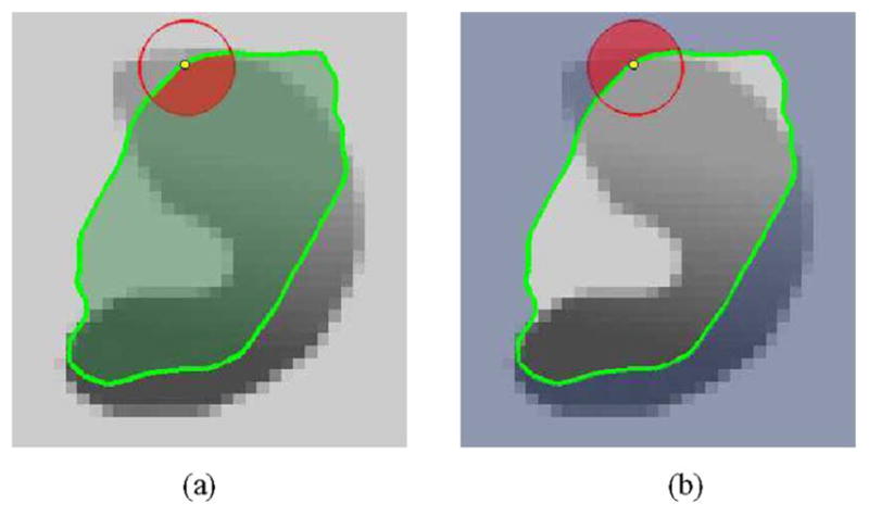
Ball is considered at each point along the contour. This ball is split by the contour into local interior and local exterior regions. In both images, the point x is represented by the small dot. The ℬ(x, y) neighborhood is represented by the larger red circle. In (a), the local interior is the shaded part of the circle and in (b), the shaded part of the circle indicates the local exterior.
The function, F is a generic internal energy measure used to represent local adherence to a given model at each point along the contour. In Section III, we examine several possible candidates for F and show how any region-based energy can be modified and rewritten as an F to be included in this framework.
In computing E, we only consider contributions from the points near the contour. By ignoring inhomogeneity that may arise far away, we give ourselves the ability to capture a much broader range of objects. In (4), we accomplish this with multiplication by the Dirac function, δφ(x) in the outer integral over x. Note that this term ensures that the curve will not change topology by spontaneously developing new contours, although it still allows for contours to split and merge. For every point x selected by δφ(x), we mask with ℬ(x, y) to ensure that F operates only on local image information about x. Thus, the total contribution of the first term of the energy is the sum of F values for every ℬ(x, y) neighborhood along the zero level set.
Finally, in order to keep the curve smooth, we add a regularization term as is commonly done. We penalize the arclength of the curve and weight this penalty by a parameter λ. The final energy is given as follows:
| (5) |
By taking the first variation of this energy with respect to φ we obtain the following evolution equation (see Appendix):
| (6) |
Notice that the only restriction on the internal energy, F is that its first variation with respect to φ can be computed. This ensures that nearly all region-based segmentation energies can be put into this framework.
III. Various Internal Energy Measures
Having formulated our framework in terms of a generic internal energy measure F, we will introduce three specific energies that can be inserted: the uniform modeling energy, the means separation energy, and the histogram separation energy. We present these energies as examples of how any energy can be improved by localization, and make no claim that one energy out performs the others in all cases. In this section, we briefly describe each global energy, give an intuitive description of its behavior, and then show how it can be incorporated into the generic framework described above.
Two well known techniques [13], [16] make use of global mean intensities of the interior and exterior regions which we as denote u and v, respectively
| (7) |
| (8) |
In Sections III-A and III-B, we will discuss internal energy functions that rely on local mean intensities to separate regions. In these sections we make use of localized equivalents of u and v defined in terms of the ℬ(x, y) function. The localized versions of the means, ux and vx
| (9) |
| (10) |
represent the intensity means in the interior and exterior of the contour localized by ℬ(x, y) at a point x. These localized statistics are needed to determine local energies at each point along the curve.
A. Uniform Modeling (UM) Energy
A well-known example of an energy that uses a constant intensity model is the Chan–Vese energy [13], which we will refer to as the uniform modeling energy
| (11) |
This energy models the foreground and background as constant intensities represented by their means, u and v. The corresponding internal energy function F is formed by replacing global means u and v by their local equivalents from (9) and (10) as follows:
| (12) |
This F can be substituted directly into (5) to form a completely localized energy. In order to obtain the evolution equation for φ, we take the derivative of F with respect to φ(y). The derivative can be written immediately as
| (13) |
By inserting this into (6), we obtain the curvature flow for the localized version of the uniform modeling energy
| (14) |
The uniform modeling flow finds its minimum energy when the interior and exterior are best approximated by means u and v. In the localized version, the minimum is obtained when each point on the curve has moved such that the local interior and exterior about every point along the curve is best approximated by local means ux and vx.
B. Mean Separation (MS) Energy
Another important global region-based energy that uses mean intensities is the one proposed by Yezzi et al. [16] which we refer to as means separation energy
| (15) |
This energy relies on the assumption that foreground and background regions should have maximally separate mean intensities. Optimizing the energy causes the curve to move so that interior and exterior means have the largest difference possible. There is no restriction on how well the regions are modeled by u and v. A corresponding F is formed by localizing the global energy with local mean equivalents as shown here
| (16) |
By substituting the derivative of FMS into (6), we obtain the following local region-based flow:
| (17) |
where Au and Av are the areas of the local interior and local exterior regions respectively given by
| (18) |
| (19) |
The optimum of this energy is obtained when ux and vx are the most different at every x along the contour. In some cases, this is more desirable than attempting to fit a constant model. Here, we are encouraging local foreground and background means to be different rather than constant. This allows this energy to find image edges very well without being distracted when interior or exterior regions are not uniform.
C. Histogram Separation (HS) Energy
Next, we consider a more complex energy that looks past simple means and compares the full histograms of the foreground and background. We show that its incorporation into the framework is as simple as the previous energies shown. Consider Pu(z) and Pv(z) to be two smoothed intensity histograms computed from the global interior and exterior regions of a partitioned image I using z intensity bins.
The Bhattacharyya coefficient, ℬ, [32] is a measure used to compare probability density functions, and results in a scalar corresponding to the similarity of the two histograms. Recently, Michailovich et al. [20] proposed an image segmentation energy
| (20) |
based on minimizing this measure. We will call this the histogram separation energy. It works by separating intensity histograms of the regions inside and outside of the curve, and thus allows interior and exterior regions to be heterogeneous as long as their intensity profiles are different.
In the localized case, Pu,x(z) and Pv,x(z) will represent the intensity histograms in the local image regions ℬ(x, y) · ℋφ(y) and ℬ(x, y) · (1 − ℋφ(y)), respectively. As before, we form the internal energy measure FHS by substituting the local equivalents for Pu(z) and Pv(z) yielding the following expression:
| (21) |
By substituting the first variation of FHS into (6), we obtain the evolution equation for the localized version of this flow
| (22) |
where K is a Gaussian kernel.
By using the Bhattacharyya measure to quantify the separation of intensity histograms, the global version of this flow is capable of segmenting objects which have nonuniform intensities. However, the intensity profile of the entire object and the entire background must still be separable. In the localized version, we remove this global constraint but remain capable of effectively separating locally nonhomogeneous regions. An example of when this property is useful is shown in the experiments in Section VI-A.
IV. Segmenting Multiple Objects
In cases where multiple foreground objects exist, simple separation into foreground and background is not sufficient. In this section, we show how to extend the proposed localized region based framework to allow simultaneous segmentation of multiple objects. We draw inspiration from the work of Brox and Weickert [31] who proposed a simple but effective algorithm for multiple region segmentation based on the idea of competing regions.
In a standard single level set evolution scheme, the energy update equation can be though of as having two competing components: advance and retreat. The advance component, a is always positive and tries to move the curve outward along its normal. Alternatively, the retreat component, r is always negative and tries to move the curve inward along its normal. The relative magnitudes of a and r govern curve evolution. Hence, the update equation for φ can be expressed as
| (23) |
To give an example, we consider the update equation for the local means separation energy in (17). This equation may be re-written in terms of the forces a and r with
| (24) |
| (25) |
Note how the length penalty used for curve regularization is included in both the a and r terms. Inclusion of this term ensures that all forces acting on the curve are represented solely by a and r.
The inherent competition of a and r in this formulation of curve evolution allows multiple signed distance functions to interact. Consider n signed distance functions, representing n evolving curves. In [31], the goal is to evolve every φi such that every point in the domain is eventually in the interior of exactly one curve. To accomplish this, each φi moves according to
| (26) |
This scheme compares the retreat portion of the typical evolutions and causes all of the curves interacting at a point to move together according to the strongest retreat force. When only one curve is present, it advances toward the uninhabited region. The simplicity of this method is appealing, and it is capable of producing complete segmentations of a scene very naturally. This behavior is well suited for global region-based energies, but a modification of this scheme is needed when used with the proposed techniques because of their local nature.
The proposed localized techniques are capable of segmenting heterogeneous objects. Thus, if they are used directly in the framework of [31] to produce complete segmentations, the proposed localized active contours could easily capture very different objects within the same contour. Specifically, the tendency of curves to advance into uninhabited areas could cause local-looking contours to move far from the intended object and fail to capture it correctly. Thus, we modify the method to work more appropriately with the proposed technique by allowing regions of the domain to remain uncovered, but continuing to prevent overlaps.
Our goal is to allow multiple contours to compete with each other at an interface, but allow them to compete with themselves when no other contours are nearby. This allows contours to stop either as they would in a single-contour framework or by competing with adjacent contours. To do this, we retain the notion of competition between advance and retreat forces and combine them in a different way to produce a new set of update equations
| (27) |
In this formulation, the advance force of the current contour is compared to the corresponding retreat forces of all adjacent contours. Similarly, the retreat force is compared to adjacent advance forces. By choosing the strongest candidates in each case, all contours at an interface will move together in order to find the best joint solution, and lone contours will continue to evolve as before. Fig. 3 shows two interacting contours and illustrates the advance and retreat forces acting on each contour.
Fig. 3.
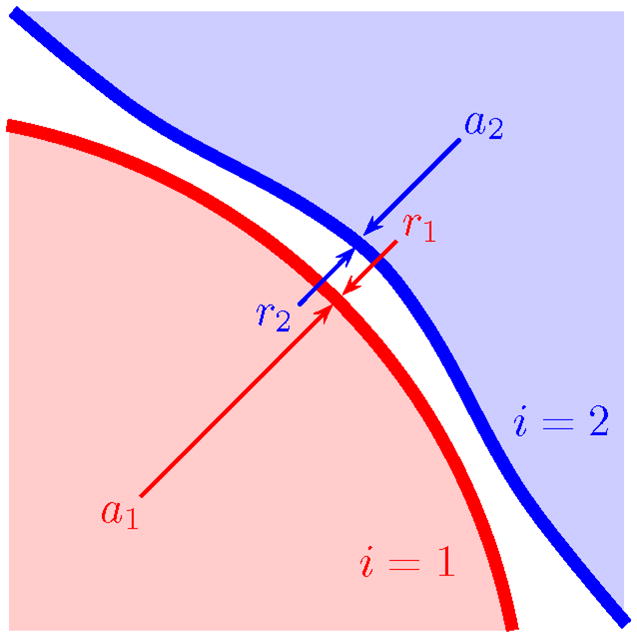
Advance, ai and retreat, ri forces are shown as they affect two interacting contours.
V. Implementation Details
We have introduced energies in terms of a signed distance function, φ. This makes it very natural to implement flows in a level set framework as proposed by [6] and [8]. In order to improve efficiency, we only compute values of φ in a narrow band around the zero level set [8]. Consequently, we re-initialize φ every few iterations using a fast marching scheme [6].
In the proposed method, local region statistics must be computed for each of the points along the evolving curve. This increases the complexity of the algorithm, and the computation time beyond that of standard global methods. Computation of local statistics is separated into two parts: initialization and updates.
The proposed local region-based method begins by initializing every pixel in the narrow band with the local interior and exterior statistics. The nature of this operation varies depending on the energy implemented. Computation of local means, for instance, is simpler than computation of local histograms. An additional cost occurs whenever the narrow band moves to include an uninitialized pixel. In this case, the local statistics of this new pixel must be initialized as well. The number of initialization operations performed is, therefore, dependent on how far from its final position the contour is initialized. The initialization operation is only performed once for each pixel and, therefore, adds a constant complexity increase. However, depending on the size of the local radius, these computations can be significant.
The update step occurs when any initialized pixel is crossed by the contour moving it from the interior to the exterior or vice versa. In our implementation we keep local statistical models in memory for every initialized pixel. When the interface crosses a pixel, the statistical models of all pixels within the neighborhood are updated. When local means are used, each pixel must maintain the number of pixels in the local regions both inside and outside of the curve as well as the sums of pixel intensities in those two regions. Updating this model consists of transferring values from the “inside” groups the “outside” groups or vice versa. For the histogram separation energy, we keep a full histogram of the local interior and exterior regions for each initialized pixel. Although this requires significantly more memory to maintain than the means model, updates are just as simple: pixel intensities are subtracted from bins of the interior histogram and added to the same bin of the associated exterior histogram or vice versa.
Compared to global methods, local methods incur a linear increase in update computation to manage all of the local statistics. This increase is proportional to the area of ℬ(x,y). Assume that at each iteration, m pixels are crossed by the moving contour, and require an update of their statistics. A global region-based method would perform m statistical updates (one for each pixel), whereas the corresponding local region-based flow would perform m · n updates where is the number of pixels that exist within the ℬ(x,y) neighborhood. Our experiments confirm this linear increase.
VI. Experiments
In order to demonstrate the strengths and limitations of the proposed localized active contours, we performed several experiments. First, we compare the three presented localized energies with their global counterparts to show the improvements offered by localization. We follow this with a demonstration of the multiple region segmentation methodology discussed in Section IV. Next, we continue with a study of the effects of local radius selection and contour initialization. Finally, we examine the speed and convergence properties of the proposed method.
A. Comparison With Global Energies
In Section III, we presented three global energies and showed how they could be localized using the framework described in this work. Here, we demonstrate the improvements that are offered by such a localization. As with all segmentation techniques, these three global techniques behave somewhat differently from one another. This is due to differences in the underlying assumptions about the given image inherent in each energy. Likewise, there are differences in the behavior of the corresponding localized energies. The purpose of the experiments given below is to demonstrate that localization can improve the performance of a given global energy, not to specifically compare the original global energies themselves. In each case, the global energies find segmentations that are consistent with their underlying assumptions about image content but are ultimately incorrect. Only the localized methods are capable of obtaining a correct segmentation in these cases.
Initially, we consider the uniform modeling energy from Section III-A. In Fig. 4, we see the benefit of localization. The localized active contour is capable of extending further to find true object boundaries in the MUSHROOM image, and is capable of stopping earlier on true object boundaries in the X-RAY image. These examples show how even images which appear simple can cause significant problems for global techniques. The slight intensity inhomogeneities present in these images prevent global region based methods from correctly capturing the objects.
Fig. 4.
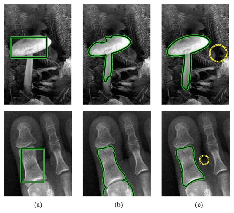
Segmentations of the MUSHROOM and X-RAY images. (a) Shows the initialization; (b) and (c) show segmentation using the global and local versions of the uniform modeling energy, respectively. The dashed yellow circle in (c) represents the localization scale. We can see a considerable improvement due to localization.
In Fig. 5, we compare the global means separation energy from Section III-B and its corresponding localization. Notice that the global energy finds only the brightest parts of the image while the localization comes to rest on object boundaries. Both the HUG image and the MONKEY image show objects and backgrounds which are multimodal, but that have intensities that change smoothly and quickly. In the HUG image in Fig. 5, the proposed method is initialized with two ellipses that correspond to a single level set. The contour changes topology as the two ellipses merge to capture both animals. The initial position of the contour (chosen to be between the two animals) is necessary in order for it to segment these holes. Because the level set is only updated in the regions specified by, it is not possible for new contours to emerge into this area.
Fig. 5.

Segmentations of the HUG and MONKEY images. (a) Shows the initialization; (b) and (c) show segmentation using the global and local versions of the means separation energy respectively. The dashed yellow circle in (c) represents the localization scale. We can see a considerable improvement due to localization.
Finally, Fig. 6 compares the global histogram separation energy from Section III-C to its localization. Again, a clear improvement is shown. While the localized contour does not capture the area between the player’s legs, the segmentation found over the rest of the player is much more accurate than in the global case. The PLAYER image shows sharp changes in intensities within the foreground. Strong edges such as the change between the player’s shirt and pants, and between the player’s socks and legs, make the localized histogram separation energy a good choice for this image. Here, the foreground is sometimes locally multimodal meaning that energies based on local means would have trouble segmenting the image.
Fig. 6.
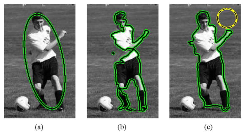
Segmentation of the PLAYER image. (a) Shows the initialization; (b) and (c) show segmentation using the global and local versions of the histogram separation energy respectively. The dashed yellow circle in (c) represents the localization scale. We can see a considerable improvement due to localization.
For consistency in these experiments, we chose λ = 0.15 in all trials to weight the influence of contour smoothness. The size of the local radius is shown by the dashed yellow circle drawn on the results for the localized methods. For results involving the global or localized histogram separation energy, 256 bins were used when computing histograms. All segmentations were allowed to run until convergence.
B. Multiple Interacting Contours
The ELEPHANTS image in Fig. 7 shows results from the method for n -ary segmentation described in Section IV. The segmentation is initialized with two contours, one on the large elephant and one on the small elephant. Each contour uses the means separation energy to find the optimal boundary. However, as the contours move they compete with themselves and with one another to ensure that they stop at the appropriate boundary and never overlap. This ensures that both elephants are captured correctly and uniquely. In the final trinary segmentation, the curves come to rest alone on certain parts of the boundaries of the elephants and together on the shared boundaries making for a reasonable segmentation result.
Fig. 7.
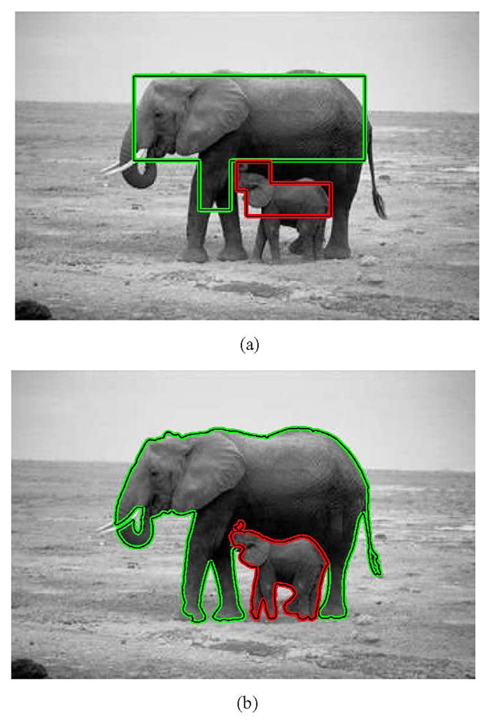
ELEPHANTS image demonstrates how two contours can interact with each other to find the correct segmentation. (a) Initialization. (b) Final result.
C. Analyzing the Localization Radius
The radius of the ball selected by the ℬ(x,y) function is an important parameter to be considered when using localized energies. Its size determines how local the resulting segmentation will be. As such, it should be chosen based on the scale of the object(s) of interest and the presence and proximity of the surrounding clutter. For example, when attempting to capture objects that are very small with nearby clutter, a small localization radius should be used. Larger radii are useful when attempting to segment large objects with less nearby clutter.
The synthetic example in Fig. 8 illustrates the effect of different localization radii. In this example, there is no reason to prefer one circle over the other as the correct segmentation. With the same initialization, it is possible to obtain two different results. By varying the radius r of the localizing ball, we can capture the local result (the smaller dark disk) or the global result (both disks together). This is a useful property for images where multiple correct segmentations may exist. Indeed, depending on the nature of the objects to be segmented the proposed method can be tuned to capture fine scale or coarse scale results.
Fig. 8.

In both images, the initialization is the same (black dashed line). However, the ball described by ℬ(x,y) (green dashed line) is optimized for small structures in (a) and larger structures in (b). Final segmentations with the means separation energy are shown by a solid yellow line. With a larger radius, a more global final solution is found than with a smaller radius.
Further, the parameter r also enforces the smoothness of statistics inside and outside the contour. The local statistics along the curve are forced to change smoothly by the fact that the ℬ(x,y) neighborhoods overlap. Thus, the larger the radius, the smoother the change in local statistics must be along the curve.
If we consider the behavior of this formulation when the radius of ℬ(x,y) is very large or very small, then we see that the ideas of local and global flows are blended together by this technique. If the proposed energy is evaluated with a very small radius, then F becomes, in essence, an edge detector based on the statistics of the pixels immediately adjacent to the center of the ball. On the other hand, if we let the radius grow such that ℬ(x,y) includes the entire image, then the local region statistics are exactly the global regions statistics and are shared by all points in the image. In this case, the behavior will be the same as the global region-based flow. Hence, by tuning the parameter r, we can choose the degree to which we blend local and global behavior.
We performed an additional experiment to show the effect of the choice of radius size on a real image. Fig. 9 shows the HEART image segmented using five different local radii. Here the desired result is to capture the bright ventricle. In the example, the smallest radius size results in an incorrect segmentation that is too local. The three intermediate radius sizes all result in accurate segmentations, and the largest radius size results in an incorrect segmentation that is too global.
Fig. 9.

(a) Shows the initialization on the HEART image; (b)–(f) show the resulting segmentations with means separation energy using localizing radius 3, 5, 7, 9, and 15, respectively. (ℬ(x,y) neighborhood shown as the dashed yellow circle in each image). Parameter λ = 0.05.
The convergence properties of these five segmentations is also of interest. The experiment in Fig. 10 reveals that the speed of convergence is often a function of radius size. The smallest radius takes the longest to converge, eventually arriving at an incorrect local optimum. The three intermediate radii converge to the same final energy, but at different speeds. The convergence speed is slower when decisions are more localized because the contour is making decisions based on less information. Finally, with the largest radius, the segmentation converges quickly to an incorrect energy value that is too global for the task at hand. Thus, this experiment demonstrates the tradeoff between speed of convergence and local radius size, and shows that radius sizes that are too big or too small may lead to incorrect segmentations.
Fig. 10.

Energies for the segmentations in Fig. 9. Energies shown (from bottom up) for radius sizes 3, 5, 7, 9, and 15 pixels. The three energies associated with intermediate radii converge to the same correct energy. The other two obtain incorrect results.
Fig. 11 illustrates some key distances that should be analyzed when choosing the size of the localization radius. In the HEART image, the desired result is the bright ventricle. Important distances to consider are those between the initialization and the desired boundary (small, blue arrows) and those between the desired boundary and nearby clutter (large, red arrows). The localization radius should be chosen so that the ℬ(x,y) neighborhood is large enough to detect the desired boundary from the initialization, but small enough that nearby clutter does not distract the contour once the desired segmentation is achieved.
Fig. 11.
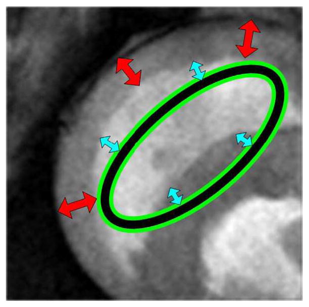
Important distances to consider when choosing the localizing radius: Small, blue arrows are the distance to the ideal result. Large, red arrows are the distance from the desired result to nearby clutter. An ideal radius size will be between the small, blue arrows and the large, red arrows.
In addition to experiments shown, we have investigated the problem of automatic scale selection. Various methods exist to detect local scale [33], [34], but we find that these methods are best suited for analyzing texture scale rather than the scale of salient objects and proximity of nearby clutter.
D. Sensitivity to Initialization
One limitation of the proposed method is that it has a greater sensitivity to initialization than global region-based methods. This is an inherent trade-off of the proposed localization. The more image data that is analyzed, the more robust the technique is against poor initialization. In other words, global methods will indeed typically be more robust to initialization than local ones. However, analyzing large amounts of image data can lead to erroneous solutions as seen in the previous experiments. Fig. 12 shows several initializations and the resulting segmentations on a synthetic image of a bimodal box.
Fig. 12.
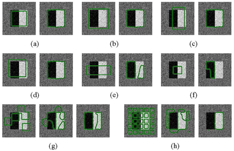
Each group shows initialization, and final segmentation with the means separation energy. Although the method is robust to some variation in initialization, it is not impervious, and should begin relatively close to the desired object boundary. (a)–(d) Correct segmentation, (c)–(h) incorrect segmentation. In these experiments, λ = 0.05 and r = 10 pixels.
Experiments (a)–(d) in Fig. 12 show a correct segmentation obtained from various initializations. Experiments (e)–(h) show incorrect segmentations. These incorrect results are due to two limitations of the technique. The first is that localized contours may not use enough information. This is shown in (f), when the contour, initialized with a small square, does not expand to fully cover the black side of the box.
The other major limitation is the “flipping” that may occur. In (h), we see that the contour is initialized with a grid of small squares. Initially, the contour finds all the borders of the box, but it finds the inside of the white side with the inside of the contour and the inside of the black side with the outside of the contour. Eventually, the part of the contour around the outside of the black side of the box collapses due to a lack of support. We notice in (g) that a similar effect occurs, but the contour partially recovers.
The increased sensitivity of the proposed method does not, however, mean that extreme care must be taken when initializing the active contours. The experiment in Fig. 13 shows magnetic resonance images (MRI) of two brains in which the corpus callosum has been segmented with several different initializations. In this experiment, the analysis of local regions allows the segmentation technique to accurately separate this structure from the rest of the brain despite its thin structure and the presence of nearby structures of similar intensity.
Fig. 13.

(a), (b) Corpus callosums from two different brains. Each row shows the initialization on the left and the final segmentation with the means separation energy on the right. Multiple initializations are shown to demonstrate robustness to initial curve placement. Parameters λ = 0.05 and r = 6 pixels for all.
E. Convergence Properties and Execution Time
Finally, we examine the convergence and timing properties of localized energies compared to the corresponding global energies. As noted in Section V, localized methods have a linear complexity increase over corresponding global methods. In our experimentation, we note that this increase is often in the range of 3 to 5 times longer when the localizing radius is on the order of 10 to 20 pixels. In Fig. 14, we compare the local and global variants of the uniform modeling energy from Section III-A and the means separation energy from Section III-B. Note that in these figures, the energies have been scaled to show them on the same graph. The actual energy values converged to are different for local and global methods. Also, note that the uniform modeling energy is minimized while the means separation energy is maximized.
Fig. 14.

(a), (c) Initialization; (b), (f) final result with global energies; (c), (g) final result with local energies; (d), (h) convergence and timing properties of localized method (dashed line) and corresponding global method (solid line).
We see that in the MUSHROOM experiment, the local and global methods both converge ≈250 in seconds. This is due to each method slowly expanding to capture the stem of the mushroom. Meanwhile, in the HUG image the global version converges to an incorrect result in ≈60 s while the local method takes ≈180 s to correctly segment the image.
In addition to the experiments shown, we implemented the proposed techniques in a fast approximate level set framework [35] which eliminates much of the overhead of curve evolution leaving statistical computations as the major computational cost. In this framework, we achieved execution times of 4 to 5 s.
VII. Conclusion
In this work, we proposed a novel framework based on localizing region-based active contours, which in certain cases has resulted in significant improvement in accuracy for segmenting heterogeneous images. We introduced several energies of this localized type and presented the steps required to localize any global region-based energy. We also demonstrated how these localized energies can interact to simultaneously segment multiple objects.
We went on to draw important conclusions from our experiments. First, we showed several illustrative examples where global region-based energies failed while the localized versions gave very reasonable segmentations. Our experiments with varying the size of the local radius demonstrated how local radii should be chosen in order to correspond to the size of salient objects and the proximity of nearby clutter. We also pointed out how convergence time decreases as radius size increases.
Next, we analyzed the limitations of the technique including its increased sensitivity to initialization compared to global methods. Finally, we performed experiments on the execution time of the proposed techniques and their global counterparts to show that while the proposed methods are slower in some cases, the speed difference is not significant for most applications.
Future work includes altering the size of the radius automatically which will remove the added parameter and allow the technique to be used with less tuning and interaction by the user. We plan to investigate using particle filtering in conjunction with variational approaches in order to accomplish this.
Finally, the ability of this type of flow to capture heterogeneous objects makes it ideal for use in some tracking applications. Many objects in realistic tracking scenarios are heterogeneous which makes frame to frame segmentation very difficult with existing methods. This segmentation approach in combination with existing contour trackers may allow these algorithms to keep track of an entire object rather than one region of homogeneous intensity.
Acknowledgments
A. Tannenbaum is supported by a Marie Curie grant through the European Unsion. This work was supported in part by grants from the NSF, AFOSR, ARO, MURI, as well as by a grant from the NIH (NAC P41 RR-13218) through Brigham and Women’s Hospital. This work is part of the National Alliance for Medical Image Computing (NAMIC), funded by the National Institutes of Health through the NIH Roadmap for Medical Research, Grant U54 EB005149. Information on the National Centers for Biomedical Computing can be obtained from http://nihroadmap.nih.gov/bioinformatics. The associate editor coordinating the review of this manuscript and approving it for publication was Prof. Peter C. Doerschuk.
The authors would like to thank S. Dambreville, D. Nain, G. Unal, and J. Malcolm for useful conversations and insights on this work.
Biographies

Shawn Lankton (S’03) is currently pursuing the Ph.D. degree at the Georgia Institute of Technology, Atlanta.
His research interests concern solving registration, segmentation, and visual tracking problems using variational optimization.

Allen Tannenbaum (M’92) is a faculty member at the Georgia Institute of Technology, Atlanta.
His research interests are in image processing, computer vision, and control.
Appendix
Derivation of Curvature Flow
Recall the first term from our original definition of E in terms of a generic internal energy F in (5)
| (28) |
To compute the first variation of this term, we start by performing a change of parameters to express E (φ) as E (φ + ξν)
| (29) |
Here, ν represents a small perturbation along the normal direction of φ weighted by a scalar ξ.
Next, we take the partial derivative of this energy with respect to ξ evaluated at ξ = 0 to represent a tiny differential of movement. By the product rule, we obtain the following:
| (30) |
Note that γφ denotes the derivative of δφ. On the zero level set, γφ evaluates to zero. As such, it does not affect the movement of the curve, and we ignore this term. Now we notice that we can move the integral over y outside the integral over x
| (31) |
At this point, we use the Cauchy–Schwartz inequality to show that the optimal direction to move φ is given by
| (32) |
Re-arranging the integrals once more gives us the same equation in a form that is easier to understand. This yields the final curve evolution
| (33) |
Contributor Information
Shawn Lankton, Email: slankton@ece.gatech.edu, Department of Electrical and Computer Engineering, Georgia Institute of Technology, Atlanta, GA 30318 USA.
Allen Tannenbaum, Email: allen.tannenbaum@ece.gatech.edu, Department of Electrical and Computer Engineering, Georgia Institute of Technology, Atlanta, GA 30318 USA, and also with the Department of Electrical Engineering, Technion—Israel Institute of Technology, Haifa, Israel.
References
- 1.Blake A, Isard M. Active Contours. Cambridge, MA: Springer; 1998. [Google Scholar]
- 2.Paragios N, Deriche R. Geodesic active contours and level sets for the detection and tracking of moving objects. IEEE Trans Pattern Anal Mach Intell. 2000 Mar;22(3):226–280. [Google Scholar]
- 3.Zhang T, Freedman D. Proc Int Conf Comput Vis. 2004. Tracking objects using density matching and shape priors; pp. 1950–1954. [Google Scholar]
- 4.Paragios N, Chen Y, Faugeras O. Handbook of Mathematial Models in Computer Vision. New York: Springer; 2005. [Google Scholar]
- 5.Morel J-M, Solimini S. Variational Methods for Image Segmentation. Boston, MA: Brikhauser; 1994. [Google Scholar]
- 6.Sethian J. Level Set Methods and Fast Marching Methods. 2. New York: Springer; 1999. [Google Scholar]
- 7.Sapiro G. Geometric Partial Differential Equations and Image Analysis. New York: Cambridge Univ. Press; 2003. [Google Scholar]
- 8.Osher S, Fedkiw R. Level Set Methods and Dynamic Implicit Surfaces. New York: Cambridge Univ. Press; 2003. [Google Scholar]
- 9.Osher S, Tsai R. Level set methods and their applications in image science. Commun Math Sci. 2003;1(4):1–20. [Google Scholar]
- 10.Kichenassamy S, Kumar A, Olver P, Tannenbaum A, AY Conformal curvature flows: From phase transitions to active vision. Arch Ration Mech Anal. 1996 Sep;134(3):275–301. [Google Scholar]
- 11.Caselles V, Kimmel R, Sapiro G. Geodesic active contours. Int J Comput Vis. 1997 Feb;22(1):61–79. [Google Scholar]
- 12.Zhu SC, Yuille A. Region competition: Unifying snakes, region growing, and bayes/mdl for multiband image segmentation. IEEE Trans Pattern Anal Mach Intell. 1996 Sep;18(9):884–900. [Google Scholar]
- 13.Chan T, Vese L. Active contours without edges. IEEE Trans Image Process. 2001 Feb;10(2):266–277. doi: 10.1109/83.902291. [DOI] [PubMed] [Google Scholar]
- 14.Yezzi A, Tsai A, Willsky A. Proc Int Conf Comput Vis. Vol. 2. 1999. A statistical approach to snakes for bimodal and trimodal imagery; pp. 898–903. [Google Scholar]
- 15.Rousson M, Deriche R. A variational framework for active and adaptive segmentation of vector valued images. Proc Workshop Motion Vid Computi. 2002:56. [Google Scholar]
- 16.Yezzi JA, Tsai A, Willsky A. A fully global approach to image segmentation via coupled curve evolution equations. J Vis Comm Image Rep. 2002 Mar;13(1):195–216. [Google Scholar]
- 17.Rousson M, Lenglet C, Deriche R. Level set and region based propagation for diffusion tensor MRI segmentation. Workshop Math. Meth. Biomed Imag. Anal; 2004. pp. 123–134. [Google Scholar]
- 18.Kim J, Fisher J, Yezzi A, Cetin M, Willsky A. A nonparametric statistical method for image segmentation using information theory and curve evolution. IEEE Trans Image Process. 2005 Oct;14(10):1486–1502. doi: 10.1109/tip.2005.854442. [DOI] [PubMed] [Google Scholar]
- 19.Cremers D, Rousson M, Deriche R. A review of statistical approaches to level set segmentation: Integrating color, texture, motion, and shape. Int J Comput Vis. 2007;72(2):195–215. [Google Scholar]
- 20.Michailovich O, Rathi Y, Tannenbaum A. Image segmentation using active contours driven by the bhattacharyya gradient flow. IEEE Trans Image Process. 2007 Nov;15(11):2787–2801. doi: 10.1109/tip.2007.908073. [DOI] [PMC free article] [PubMed] [Google Scholar]
- 21.Paragios N, Deriche R. Geodesic active regions: A new framework to deal with frame partition problems in computer vision. Int J Comput Vis. 2002 Feb;46(3):223–247. [Google Scholar]
- 22.Sum K, Cheung P. A novel active contour model using local and global statistics for vessel extraction. Proc Eng Medicine Bio Soc. 2006:3126–3129. doi: 10.1109/IEMBS.2006.260817. [DOI] [PubMed] [Google Scholar]
- 23.Sum K, Cheung P. Vessel extraction under non-uniform illumination: A level set approach. IEEE Trans Biomed Eng. 2008 Jan;55(1):358–360. doi: 10.1109/TBME.2007.896587. [DOI] [PubMed] [Google Scholar]
- 24.Brox T, Cremers D. On the statistical interpretation of the piecewise smooth mumfordshah functional. Proc Scale Space Var Met Comp Vis. 2007;4485:203–213. [Google Scholar]
- 25.Mumford D, Shah J. Optimal approximations by piecewise smooth functions and associated variational problems. Comm Pure Appl Math. 1989;42:577–685. [Google Scholar]
- 26.Mumford D. A bayesian rationale for energy functionals. In: Romeny B, editor. Geometry Driven Diffusion in Computer Vision. Dor-drecht, The Netherlands: Kluwer; 1994. pp. 141–153. [Google Scholar]
- 27.Li C, Kao C-Y, Gore JC, Ding Z. Implicit active contours driven by local binary fitting energy. presented at the Comput. Vis. Pattern Recog; Jun, 2007. [Google Scholar]
- 28.Piovano J, Rousson M, Papadopoulo T. Efficient segmentation of piecewise smooth images. Proc Scale Space Var Met Comp Vis. 2007;4485:709–720. [Google Scholar]
- 29.An J, Rousson M, Xu C. γ-convergence approximation to piecewise smooth medical image segmentation. Proc Med Imag Comput Comp Assist Interven. 2007;4792:495–502. doi: 10.1007/978-3-540-75759-7_60. [DOI] [PubMed] [Google Scholar]
- 30.Lankton S, Nain D, Yezzi A, Tannenbaum A. Hybrid geodesic region-based curve evolutions for image segmentation. Proc SPIE: Med Imag. 2007 Mar;6510:65104U. [Google Scholar]
- 31.Brox T, Weickert J. Level set segmentation with multiple regions. IEEE Trans Image Process. 2006 Oct;15(10):3213–3218. doi: 10.1109/tip.2006.877481. [DOI] [PubMed] [Google Scholar]
- 32.Bhattacharyya A. On a measure of divergence between two statistical populations dened by their probability distributions. Bull Calcutta Math Soc. 1943;35:99–110. [Google Scholar]
- 33.Elder J, Zucker S. Local scale control for edge detection and blur estimation. IEEE Trans Pattern Anal Mach Intell. 1998 Jul;20(7):699–716. [Google Scholar]
- 34.Brox T, Weickert J. A tv flow based local scale estimate and its application to texture discrimination. J Vis Commun Image R. 2006;17:1053–1073. [Google Scholar]
- 35.Malcolm J, Rathi Y, Yezzi A, Tannenbaum A. Fast approximate surface evolution in arbitrary dimension. presented at the SPIE Med. Imag; 2008. [DOI] [PMC free article] [PubMed] [Google Scholar]