Simulation-based model selection for dynamical systems in systems and population biology

Abstract

Motivation: Computer simulations have become an important tool across the biomedical sciences and beyond. For many important problems several different models or hypotheses exist and choosing which one best describes reality or observed data is not straightforward. We therefore require suitable statistical tools that allow us to choose rationally between different mechanistic models of, e.g. signal transduction or gene regulation networks. This is particularly challenging in systems biology where only a small number of molecular species can be assayed at any given time and all measurements are subject to measurement uncertainty.

Results: Here, we develop such a model selection framework based on approximate Bayesian computation and employing sequential Monte Carlo sampling. We show that our approach can be applied across a wide range of biological scenarios, and we illustrate its use on real data describing influenza dynamics and the JAK-STAT signalling pathway. Bayesian model selection strikes a balance between the complexity of the simulation models and their ability to describe observed data. The present approach enables us to employ the whole formal apparatus to any system that can be (efficiently) simulated, even when exact likelihoods are computationally intractable.

Contact: ttoni@imperial.ac.uk; m.stumpf@imperial.ac.uk

Supplementary information: Supplementary data are available at Bioinformatics online.

1 INTRODUCTION

Mathematical models are widely used to describe and analyse complex systems and processes. Formulating a model to describe, e.g. a signalling pathway or host parasite system, requires us to condense our assumptions and knowledge into a single coherent framework (May, 2004). Mathematical analysis and computer simulations of such models then allow us to compare model predictions with experimental observations in order to test, and ultimately improve these models. The continuing success, e.g. of systems biology, relies on the judicious combination of experimental and theoretical lines of argument.

Because many of the mathematical models in biology (as in many other disciplines) are too complicated to be analysed in a closed form, computer simulations have become the primary tool in the quantitative analysis of very large or complex biological systems. This, however, can complicate comparisons of different candidate models in light of (frequently sparse and noisy) observed data. Whenever probabilistic models exist, we can employ standard model selection approaches of either a frequentist, Bayesian or information theoretic nature (Burnham and Anderson, 2002; Vyshemirsky and Girolami, 2008). But if suitable probability models do not exist, or if the evaluation of the likelihood is computationally intractable, then we have to base our assessment on the level of agreement between simulated and observed data. This is particularly challenging when the parameters of simulation models are not known but must be inferred from observed data as well. Bayesian model selection side-steps or overcomes this problem by marginalizing (i.e. integrating) over model parameters, thereby effectively treating all model parameters as nuisance parameters.

For the case of parameter estimation when likelihoods are intractable, approximate Bayesian computation (ABC) frameworks have been applied successfully (Beaumont et al., 2002; Marjoram et al., 2003; Ratmann et al., 2007, 2009; Sisson et al., 2007; Toni et al., 2009). In ABC, the calculation of the likelihood is replaced by a comparison between the observed data and simulated data. Given the prior distribution P(θ) of parameter θ, the goal is to approximate the posterior distribution, P(θ|D₀)∝f(D₀|θ)P(θ), where f(D₀|θ) is the likelihood of θ given the data D₀. ABC methods have the following generic form:

1. Sample a candidate parameter vector θ^* from prior distribution P(θ).

2. Simulate a dataset D^* from the model described by a conditional probability distribution f(D|θ^*).

3. Compare the simulated dataset, D^*, to the experimental data, D₀, using a distance function, d, and tolerance ϵ; if d(D₀, D^*)≤ϵ, accept θ^*. The tolerance ϵ≥0 is the desired level of agreement between D₀ and D^*.

The output of an ABC algorithm is a sample of parameters from the distribution P(θ|d(D₀, D^*)≤ϵ). If ϵ is sufficiently small then this distribution will be a good approximation for the ‘true’ posterior distribution, P(θ|D₀). A tutorial on ABC methods is available in the Supplementary Material.

Such a parameter estimation approach can be used whenever the model is known. However, when several plausible candidate models are available we have a model selection problem, where both the model structure and parameters are unknown. In the Bayesian framework, model selection is closely related to parameter estimation, but the focus shifts onto the marginal posterior probability of model m given data D₀,

where P(D₀|m) is the marginal likelihood and P(m) the prior probability of the model (Gelman et al., 2003). This framework has some conceptual advantages over classical hypothesis testing: for example, we can rank an arbitrary number of different non-nested models by their marginal probabilities; and rather than only considering evidence against a model the Bayesian framework also weights evidence in a model's favour (Jeffreys, 1939). In practical applications, however, a range of potential pitfalls need considering: model probabilities can show strong dependence on model and parameter priors; and the computational effort needed to evaluate these posterior distributions can make these approaches cumbersome.

The computationally expensive step in Bayesian model selection is the evaluation of the marginal likelihood, which is obtained by marginalizing over model parameters; i.e. P(D₀|m)=∫f(D₀|m, θ)P(θ|m)dθ, where P(θ|m) is the parameter prior for model m. Here, we develop a computationally efficient ABC model selection formalism based on a sequential Monte Carlo (SMC) sampler. We show that our ABC SMC procedure allows us to employ the whole paraphernalia of the Bayesian model selection formalism, and illustrate the use and scope of our new approach in a range of models: chemical reaction dynamics, Gibbs random fields and real data describing influenza spread and JAK-STAT signal transduction.

2 ABC FOR MODEL SELECTION

Our goal is to estimate the marginal posterior distribution of a model, P(m|D₀), and in this section we explain two ways in which this problem can be approached. In the joint space-based approach, we define a joint space of model indicators, m=1, 2,…, |ℳ|, and corresponding model parameters, θ, obtain the joint posterior distribution over the combined space of models and parameters, P(θ, m|D₀), and finally marginalize over parameters to obtain P(m|D₀). In the second, marginal likelihood-based approach, we estimate marginal likelihoods (also called the evidence), P(D₀|m), for each given model, and use these to calculate the marginal posterior model distributions through

Both approaches have been applied under the ABC rejection scheme, which is computationally prohibitive for models with even an only moderate number of parameters (Grelaud et al., 2009; Wilkinson, 2007). Here, we incorporate ideas from SMC to both of the above approaches, making them computationally more efficient. In this section, we present only the more powerful approach ABC SMC model selection on the joint space. We refer the reader to the Supplementary Material for derivations and details, as well as discussion on the ABC SMC model selection algorithm based on the marginal likelihood approach.

In model selection based on ABC rejection, we adapt the basic ABC procedure (presented in Section 1) to the joint space, where particles (m, θ) consist of a model indicator m and a parameter θ. The ABC rejection model selection algorithm on the joint space proceeds as follows (Grelaud et al., 2009):

1. Draw m^* from the prior P(m).

2. Sample θ^* from the prior P(θ|m^*).

3. Simulate a candidate dataset D^* ∼ f(D|θ^*, m^*).

4. Compute the distance. If d(D₀, D^*)≤ϵ, accept (m^*, θ^*), otherwise reject it.

5. Return to 1.

Once a sample of N particles has been accepted, the marginal posterior distribution is approximated by

In the ABC SMC model selection algorithm on the joint space, particles (parameter vectors) {(m₁, θ₁),…, (m_N, θ_N)} are sampled from the prior distribution, P(m, θ), and propagated through a sequence of intermediate distributions, P(m, θ|d(D₀, D^*)≤ϵ_i), i=1,…, T − 1, until they represent a sample from the target distribution, P(m, θ|d(D₀, D^*)≤ϵ_T). The tolerances ϵ_i are chosen such that ϵ₁>···>ϵ_T≥0, and the distributions thus gradually evolve towards the target posterior distribution.

The algorithm is presented below (and explained in the Supplementary Material).

2.1 ABC SMC model selection algorithm on the joint space

• MS1 Initialize ϵ₁,…, ϵ_T.

  Set the population indicator t=1.

• MS2.0 Set the particle indicator i=1.

• MS2.1 If t=1, sample (m^**, θ^**) from the prior distribution P(m, θ).

  If t> 1, sample m^* with probability P_t−1(m^*) and draw m^** ∼ KM_t (m|m^*).

  Sample θ^* from previous population {θ(m^**)_t−1} with weights w_t−1 and draw θ^** ∼ KP_t,m^**(θ|θ^*).

  If P(m^**, θ^**)=0, return to MS2.1.

  Simulate a candidate dataset D^* ∼ f(D|θ^**, m^**).

  If d(D₀, D^*)>ϵ_t, return to MS2.1.

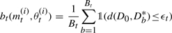
• MS2.2 Set (m_t⁽ⁱ⁾, θ_t⁽ⁱ⁾)=(m^**, θ^**) and calculate the weight of the particle as

  

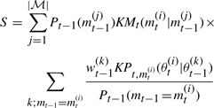
  where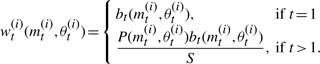

  

  

  If i<N set i=i+1, go to MS2.1.

• MS3 Normalize the weights w_t.

  Sum the particle weights to obtain marginal model probabilities,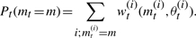

  

  If t<T, set t=t+1, go to MS2.0.

Particles sampled from a previous distribution are denoted by a single asterisk, and after perturbation by a double asterisk. KM is a model perturbation kernel which allows us to obtain model m from model m^* and KP is the parameter perturbation kernel. B_t≥1 is the number of replicate simulation run for a fixed particle (for deterministic models B_t=1) and |ℳ| denotes the number of candidate models.

The output of the algorithm, i.e. the set of particles {(m_T, θ_T)} associated with weights w_T, is the approximation of the full posterior distribution on the joint model and parameter space. The approximation of the marginal posterior distribution of the model obtained by marginalization is

and we can also straightforwardly obtain the marginalized parameter distributions.

The algorithm requires the user to define the prior distribution, distance function, tolerance schedule and perturbation kernels. In all the examples presented in the results section, we choose uniform prior distributions for all parameters and models; that is, all models are a priori equally plausible. Such priors are informative in a sense that they define a feasible parameter region (e.g. reaction rates are positive), but they are predominantly non-informative as they do not specify any further preference for particular parameter values. This way the inference will mostly be informed by the information contained in the data. A good tolerance can be found empirically by trying to reach the lowest distance feasible and arrive at the posterior distribution in a computationally efficient way. Our perturbation kernels are component-wise truncated uniform or Gaussian and are automatically adapted by feeding back information on the obtained parameter ranges from the previous population. Distance functions are defined for each model as specified in Section 3. The algorithm presented in Toni et al. (2009) is a special case of the above algorithm for discrete uniform KM kernel and uniform prior distribution of the model P(m).

3 RESULTS

In this section, we illustrate ABC SMC for model selection on a simple example of stochastic reaction kinetics. We then compare the computational efficiency of ABC SMC for stochastic models of Gibbs random fields with that of the ABC rejection model selection method. Finally, we apply the algorithm to several real datasets: first, we select between different stochastic models of influenza epidemics (where we can compare our approach with previously published results obtained using exact Bayesian model selection), and then apply our approach to choose from among different mechanistic models for the STAT5 signalling pathway.

3.1 Chemical reaction kinetics

We illustrate our algorithm for the stochastic reaction kinetic models and . The first is a model of an autocatalytic reaction, where the reaction product Y is the catalyst for the reaction. In the second, molecules Y do not need to be present for a change from X to Y to occur. Such models have, for example, been considered in the context of prion replication dynamics (Eigen, 1996; Prusiner, 1982), where X represents a healthy form of a prion protein and Y a diseased form.

We simulate synthetic datasets of Y measured at 20 time points using Gillespie algorithm (Gillespie, 1977) from model 2 with parameter k₂=30 and initial conditions X₀=40, Y₀=3 (Fig. 1a; Supplementary Table 1). We apply our ABC SMC algorithm for model selection, which identifies the correct model with high confidence (Fig. 1b).

Fig. 1.

(a) Stochastic trajectories of species X (red) and Y (blue). Model 1 is simulated for k₁=2.1 (dashed line), model 2 for k₂=30 (full line). Data points are represented by circles. (b) We have repeated the model selection run 20 times; the red sections present 25% and 75% quantiles around the median. Prior distribution P(m) is chosen uniform and k₁, k₂ ∼ U(0, 100). Perturbation kernels are chosen as follows: KP_t(k|k^*)=U(−σ, σ), σ=2 (max{k}_t−1−min{k}_t−1) and KM_t(m|m^*)=0.7 if m=m^* and 0.3 otherwise. Number of particles N=1000. B_t=1. Distance function is mean squared error and tolerance schedule ϵ={3000, 1400, 600, 140, 40}.

3.2 Gibbs random fields

Gibbs random fields have become staple models in machine learning, including applications in computational biology and bioinformatics [see, e.g. Grelaud et al. (2009); Wei and Li (2007)]. Here, we use two Gibbs random field models (Møller, 2003), for which closed form posterior distributions are available. This allows us to compare the ABC SMC approximated posterior distributions of the models with true posterior distributions, and to demonstrate the computational efficiency of our approach when compared with model selection based on ABC rejection sampling.

Both models, m₀ and m₁, are defined on a sequence of n binary random variables, x=(x₁,…, x_n), x_i∈{0, 1}; m₀ is a collection of n i.i.d. Bernoulli random variables with probability θ₀/(1+exp(θ₀)); m₁ is equivalent to a standard Ising model, i.e. x₁ is taken to be a binary random variable and P(x_i+1=x_i|x_i)=θ₁/(1+exp(θ₁)) for i=2,…, x_n. The likelihood functions are

where S₀(x)=∑_i=1ⁿ 1(x_i = 1) and S₁(x)=∑_i=2ⁿ 1(x_i=x_i−1) are sufficient statistics, respectively.

We simulate 1000 datasets from both models for different values of parameters θ₀ ∼ U(−5, 5), θ₁ ∼ U(0, 6) and n=100. Using ABC SMC for model selection allows us to estimate posterior model distributions correctly and demonstrate a considerable computational speed-up in ABC SMC compared with ABC rejection (Fig. 2).

Fig. 2.

(a) True versus inferred posterior distribution of model m₀. In ABC SMC, we use the Euclidian distance . N=500. B_t=1. Tolerance schedule: ϵ={9, 4, 3, 2, 1, 0}. Perturbation kernels: KM_t(m|m^*)=0.75 if m=m^* and 0.25 otherwise; KP_t(θ|θ^*)=U(−σ, σ), σ=0.5 (max{θ}_t−1−min{θ}_t−1). We have excluded those datasets for which all states are in 0 or 1 (for which P(m=0)≈0.3094 is also correctly inferred) from the analysis. (b) Comparison of the number of simulation steps needed by ABC rejection (n_Rej) and ABC SMC (n_SMC); ABC SMC yields ∼50-fold speed-up on average.

3.3 Infuenza infection outbreaks

We next apply ABC SMC for model selection to models of the spread of different strains of the influenza virus. We use data from influenza A (H3N2) outbreaks that occurred in 1977–1978 and 1980–1981 in Tecomseh, Michigan (Addy et al., 1991, Supplementary Table 2), and a second dataset of an influenza B infection outbreak in 1975–1976 and influenza A (H1N1) infection outbreak in 1978–1979 in Seattle, Washington (Longini and Koopman, 1982, Supplementary Table 3). The basic questions to be addressed here are whether (i) different outbreaks of the same strain and (ii) outbreaks of different molecular strains of the influenza virus can be described by the same model of disease spread.

We assume that virus can spread from infected to susceptible individuals and distinguish between spread inside households or across the population at large (Longini and Koopman, 1982). Let q_c denote the probability that a susceptible individual does not get infected from the community and q_h the probability that a susceptible individual escapes infection within their household. Then w_js, the probability that j out of the s susceptibles in a household become infected, is given by

(1)

where w_0s=q_c^s, s=0, 1, 2,… and w_jj=1−∑_i=0^j−1w_ij. We are interested in inferring the pair of parameters q_h and q_c of the model (1) using the data from Supplementary Table 2. These data were obtained from two separate outbreaks of the same strain, H3N2, and the question of interest is whether these are characterized by the same epidemiological parameters [this question was previously considered in Clancy and O'Neill (2007) and O'Neill et al. (2000)]. To investigate this issue, we consider two models: one with four parameters, q_h1, q_c1, q_h2, q_c2, which describes the hypothesis that each outbreak has its own characteristics; the second models the hypothesis that both outbreaks share the same epidemiological parameter values for q_h and q_c. Prior distributions of all parameters are chosen to be uniform over the range [0, 1].

To apply ABC SMC, we use a distance function

where ‖ ‖_F denotes the Frobenious norm, D₀=D₁∪D₂ with D₁ the 1977–1978 outbreak and D₂ the 1980–1981 outbreak datasets from Supplementary Table 2, and D^* is the simulation output from model (1). The results we obtain are summarized in Figure 3a and b and strongly suggest that the two outbreaks appear to have shared the same epidemiological characteristics. Figure 3a shows the posterior distribution of the four-parameter model. The marginal posterior distributions of q_h1 and q_c1 are largely overlapping with the marginal posterior distributions of q_h2 and q_c2 and we therefore, unsurprisingly, get strong evidence in favour of the two-parameter model. Figure 3b shows the marginal posterior distribution of the model; the posterior probability of model 1 is 0.98 (median over 10 runs), which gives unambiguous support to model 1, meaning that outbreaks of the same strain share the same dynamics.

Fig. 3.

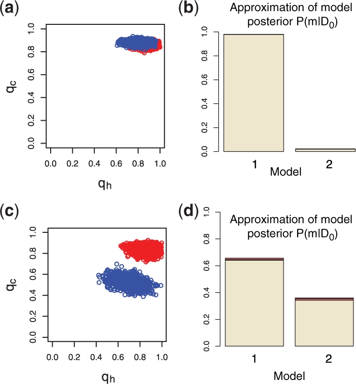
(a) ABC SMC posterior distributions for parameters inferred for a four-parameter model from the data in Supplementary Table 2. Marginal posterior distributions of parameters q_c1, q_h1 (red) and q_c2, q_h2 (blue). (b) Approximation of a posterior marginal distribution P(m|D₀). Model 1 is a two-parameter and model 2 a four-parameter model (1). All intermediate populations are shown in Supplementary Figure 1a. (c) The same as (a) but here the data used is from Supplementary Table 3. (d) Estimation of a posterior marginal distribution. Model 1 is a two-parameter and model 2 a three-parameter model (1). All intermediate populations are shown in Supplementary Figure 1b.

Outbreaks due to a different viral strain (Supplementary Table 3) have different characteristics as indicated by the posterior distribution of the four-parameter model presented in Figure 3c. This was confirmed by applying our model selection algorithm; the inferred posterior marginal model probability of a two-parameter model was negligible (data not shown). From Figure 3c, we also see that these differences are due to differences in viral spread across the community whereas within-household dynamics are comparable. We thus explore a further model with three parameters, q_c1, q_c2, q_h (model 1), where the two outbreaks share the same within-household characteristics (q_h), and compare it against and the four-parameter model (model 2). The obtained Bayes factor suggests that there is only very week evidence in favour of model 1 (Fig. 3d), which is in agreement with the result of Clancy and O'Neill (2007).

In general genetic predisposition, differences in immunity and lifestyle, etc., will lead to heterogeneity in susceptibility to viral infection among the host population. Such a model can be written as (O'Neill et al., 2000)

(2)

On the basis of the previous results, we combine both outbreak datasets from Supplementary Table 2, and find some evidence that model (1) explains the data better than model (1), suggesting that the host-virus dynamics are shaped by the molecular nature of the viral strain, as well as by variability in the host population (Supplementary Fig. 2).

3.4 JAK-STAT signalling pathway

Having convinced ourselves that the novel ABC SMC model selection approach agrees with the analytical model probabilities and those obtained using conventional Bayesian model selection, while outperforming conventional ABC rejection model selection approaches, we can now turn our attention to real world scenarios that have not previously been considered from a Bayesian (exact or approximate) perspective. Here, we consider models of signalling though the erythropoietin receptor (EpoR), transduced by STAT5 (Fig. 4a) (Darnell, 1997; Horvath, 2000). Signalling through this receptor is crucial for proliferation, differentiation and survival of erythroid progenitor cells (Klingmüller et al., 1996). When the Epo hormone binds to the EpoR receptor, the receptor's cytoplasmic domain is phosporylated, which creates a docking site for signalling molecules, in particular STAT5. Upon binding to the activated receptor, STAT5 first becomes phosphorylated, then dimerizes and translocates to the nucleus, where it acts as a transcription factor. There have been competing hypotheses about what happens with the STAT5 in the nucleus. Originally, it had been suggested that STAT5 gets degraded in the nucleus in an ubiquitin-associated way (Kim and Maniatis, 1996), but other evidence suggests that they are dephosphorylated in the nucleus and then trafficked back to the cytoplasm (Köster and Hauser, 1999).

Fig. 4.

(a) STAT5 signalling pathway. Adapted from (Arbouzova and Zeidler, 2006). (b) Histograms show populations of the model parameter m. Population 20 represents the approximation of the marginal posterior distribution of m. Tolerance schedule: ϵ={200, 100, 50, 35, 30, 25, 22, 20, 19, 18, 17, 16, 15, 14, 13, 12, 11, 10, 9, 8}. Perturbation kernels: KM_t(m|m^*)=0.6 if m=m^* and 0.2 otherwise; KP_t(θ|θ^*)=U(−σ, σ), σ=0.5 (max{θ}_t−1−min{θ}_t−1). N=500. Distance function: 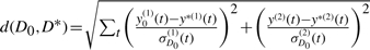, with D₀={y₀⁽¹⁾, y₀⁽²⁾}, D^*={y^*(1), y^*(2)} and y⁽¹⁾ the total amount of phosphoryalated STAT5 in the cytoplasm and y⁽²⁾ the total amount of STAT5 in the cytoplasm. σ_D0⁽¹⁾ and σ_D0⁽²⁾ are the associated confidence intervals; reassuringly, other distance functions, e.g. the square root of the sum of squared errors yield identical model selection results (data not shown).

The ambiguity of the shutoff mechanism of STAT5 in the nucleus triggered the development of several mathematical models (Müller et al., 2004; Swameye et al., 2003; Timmer and Müller, 2004) describing different hypotheses. All models assume mass action kinetics and denote the amount of activated Epo-receptors by EpoR_A, monomeric unphosphorylated and phosphorylated STAT5 molecules by x₁ and x₂, respectively, dimeric phosphorylated STAT5 in the cytoplasm by x₃ and dimeric phosphorylated STAT5 in the nucleus by x₄. The most basic model developed by Timmer et al., under the assumption that phosphorylated STAT5 does not leave the nucleus, consists of the following kinetic equations,

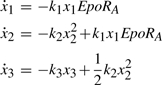(3)

(4)

One can then assume that phosphorylated STAT5 dimers dissociate and leave the nucleus; this is modelled by adding appropriate kinetic terms to the Equations (3) and (4) of the basic model to obtain

The cycling model can be developed further by assuming a delay before STAT5 leaves the nucleus:

(5)

This model was chosen as the best model in the original analyses (Müller et al., 2004; Swameye et al., 2003) based on a numerical evaluation of the likelihood, followed by a likelihood ratio test and bootstrap procedure for model selection. The data are partially observed time course measurements of the total amount of STAT5 in the cytoplasm, and the amount of phosphorylated STAT5 in the cytoplasm; both are only known up to a normalizing factor.

We propose a further model with clear physical interpretation where the delay acts on STAT5 inside the nucleus (x₄) rather than on x₃ [in Equation (5)], for which a biological interpretation is difficult. Instead of x₃(t−τ), we propose to model the delay of phosphorylated STAT5 x₄ in the nucleus directly and obtain (Zi and Klipp, 2006):

We perform the ABC SMC model selection algorithm on the following non-nested models: (i) cycling delay model with x₃(t−τ), (ii) cycling delay model with x₄(t−τ) and (iii) cycling model without a delay. The model parameter m can therefore take values 1–3.

For each proposed model and parameter combination we numerically solve the ordinary differential equations and add ϵ ∼ N(0, σ) to obtain the simulated time course data. The noise parameter σ can be either fixed or treated as another parameter to be estimated; we consider the latter option, under the assumption that the experimental noise is independent and identically distributed for all time points.

Figure 4b shows intermediate populations leading to the ABC SMC marginal posterior distribution over the model parameters m (population 20). Bayes factors can be calculated from the last population and according to the conventional interpretation of Bayes factors (Kass and Raftery, 1995), it can be concluded that there is strong evidence in favour of model 3 compared to model 1, positive evidence in favour of model 3 compared to model 2, and positive evidence in favour of model 2 compared to model 1. Thus, cycling appears to be clearly important and the model that receives the most support is the cycling model without a time delay. Here, the flexibility of ABC SMC has allowed us to perform simultaneous model selection on non-nested models of ordinary and time-delay differential equations.

4 DISCUSSION

We have developed a novel model selection methodology based on ABC and SMC. The results obtained here illustrate the usefulness and wide applicability of our ABC SMC method, even when experimental data are scarce, when no measurements are available for some species, when temporal data are not measured at equidistant time points and when parameters such as kinetic rates are unknown. In the context of dynamical systems, our method can be applied across all simulation and modelling (including qualitative modelling) frameworks; for JAK-STAT signal transduction dynamics, for example, we have been able to compare the relative explanatory power of ordinary and time-delay differential equation models. Our model selection procedure is also not confined to dynamical systems; in fact the scope for application is immense and limited only by the availability of efficient simulation approaches.

Routine application to complex models in systems, computational and population biology with hundreds or thousands of parameters (Chen et al., 2009), will require further numerical developments due to the high-computational cost of repeated simulations. SMC-based ABC methods are, however, highly parallelizable and we believe that future work should exploit this property to make these methods computationally more efficient. Further potential improvements might come from (i) regression adjustment techniques that have so far been applied in the parameter estimation ABC framework (Beaumont et al., 2002; Blum and François, 2009; Excoffier, 2009); (ii) from automatic generation of the tolerance schedules (Del Moral et al., 2009); and (iii) by developing more sophisticated perturbation kernels that exploit inherent properties of biological dynamical systems such as sloppiness (Gutenkunst et al., 2007; Secrier et al., 2009); here especially we feel that there is substantial room for improvement as the likelihoods of dynamical systems contain information about the qualitative behaviour (Kirk et al., 2008) which can also be exploited in ABC frameworks.

5 CONCLUSIONS

We conclude by emphasizing the need for inferential methods which can assess the relative performance and reliability of different models. The need for such reliable model selection procedures can hardly be overstated: with an increasing number of biomedical problems being studied using simulation approaches, there is an obvious and urgent need for statistically sound approaches that allow us to differentiate between different models. If parameters are known or the likelihood is available in a closed form, then the model selection is generally straightforward. However, for many of the most interesting systems biology (and generally, scientific) problems this is not the case and here ABC SMC can be employed.

REFERENCES

- Addy C, Jr, et al. A generalized stochastic model for the analysis of infectious disease final size data. Biometrics. 1991;47:961–974. [PubMed] [Google Scholar]
- Arbouzova NI, Zeidler MP. JAK/STAT signalling in drosophila: insights into conserved regulatory and cellular functions. Development. 2006;133:2605–2616. doi: 10.1242/dev.02411. [DOI] [PubMed] [Google Scholar]
- Beaumont MA, et al. Approximate Bayesian computation in population genetics. Genetics. 2002;162:2025–2035. doi: 10.1093/genetics/162.4.2025. [DOI] [PMC free article] [PubMed] [Google Scholar]
- Blum MG, François O. Non-linear regression models for approximate Bayesian computation. Stat. Comput. 2009 [Epub ahead of print, doi:10.1007/s11222-009-9116-0] [Google Scholar]
- Burnham K, Anderson D. Model Selection and Multimodel Inference: A Practical Information-Theoretic Approach. New York: Springer; 2002. [Google Scholar]
- Chen WW, et al. Input-output behavior of ErbB signaling pathways as revealed by a mass action model trained against dynamic data. Mol. Syst. Biol. 2009;5:239. doi: 10.1038/msb.2008.74. [DOI] [PMC free article] [PubMed] [Google Scholar]
- Clancy D, O'Neill PD. Exact Bayesian inference and model selection for stochastic models of epidemics among a community of households. Scand. J. Stat. 2007;34:259–274. [Google Scholar]
- Darnell JE. STATs and gene regulation. Science. 1997;277:1630–1635. doi: 10.1126/science.277.5332.1630. [DOI] [PubMed] [Google Scholar]
- Del Moral P, et al. An adaptive sequential Monte Carlo method for approximate Bayesian computation. Imperial College Technical Report; 2009. [Google Scholar]
- Eigen M. Prionics or the kinetic basis of prion diseases. Biophys. Chem. 1996;63:A1–A18. doi: 10.1016/s0301-4622(96)02250-8. [DOI] [PubMed] [Google Scholar]
- Excoffier CLDWL. Bayesian computation and model selection in population genetics. 2009 arXiv:0901.2231v1 [stat.ME] [Google Scholar]
- Gelman A, et al. Bayesian Data Analysis. 2. London: Chapman & Hall/CRC; 2003. [Google Scholar]
- Gillespie D. Exact stochastic simulation of coupled chemical reactions. J. Phys. Chem. 1977;81:2340–2361. [Google Scholar]
- Grelaud A, et al. ABC likelihood-free methods for model choice in Gibbs random fields. Bayesian Anal. 2009;4:317–336. [Google Scholar]
- Gutenkunst R, et al. Universally sloppy parameter sensitivities in systems biology models. PLoS Comput. Biol. 2007;3:e189. doi: 10.1371/journal.pcbi.0030189. [DOI] [PMC free article] [PubMed] [Google Scholar]
- Horvath CM. STAT proteins and transcriptional responses to extracellular signals. Trends Biochem. Sci. 2000;25:496–502. doi: 10.1016/s0968-0004(00)01624-8. [DOI] [PubMed] [Google Scholar]
- Jeffreys H. Theory of Probability. 1st. Oxford: The Clarendon Press; 1939. [Google Scholar]
- Kass R, Raftery A. Bayes factors. J. Am. Stat. Assoc. 1995;90:773–795. [Google Scholar]
- Kim TK, Maniatis T. Regulation of interferon-gamma-activated STAT1 by the ubiquitin-proteasome pathway. Science. 1996;273:1717–1719. doi: 10.1126/science.273.5282.1717. [DOI] [PubMed] [Google Scholar]
- Kirk PDW, et al. Parameter inference for biochemical systems that undergo a Hopf bifurcation. Biophys. J. 2008;95:540–549. doi: 10.1529/biophysj.107.126086. [DOI] [PMC free article] [PubMed] [Google Scholar]
- Klingmüller U, et al. Multiple tyrosine residues in the cytosolic domain of the erythropoietin receptor promote activation of STAT5. Proc. Natl Acad. Sci. USA. 1996;93:8324–8328. doi: 10.1073/pnas.93.16.8324. [DOI] [PMC free article] [PubMed] [Google Scholar]
- Köster M, Hauser H. Dynamic redistribution of STAT1 protein in IFN signaling visualized by GFP fusion proteins. Eur. J. Biochem. 1999;260:137–144. doi: 10.1046/j.1432-1327.1999.00149.x. [DOI] [PubMed] [Google Scholar]
- Longini IL, Jr., Koopman J. Household and community transmission parameters from final distributions of infections in households. Biometrics. 1982;38:115–126. [PubMed] [Google Scholar]
- Marjoram P, et al. Markov chain Monte Carlo without likelihoods. Proc. Natl Acad. Sci. USA. 2003;100:15324–15328. doi: 10.1073/pnas.0306899100. [DOI] [PMC free article] [PubMed] [Google Scholar]
- May RM. Uses and abuses of mathematics in biology. Science. 2004;303:790–793. doi: 10.1126/science.1094442. [DOI] [PubMed] [Google Scholar]
- Möller J. Spatial Statistics and Computational Methods. New York: Springer; 2003. [Google Scholar]
- Müller TG, et al. Tests for cycling in a signalling pathway. J. R. Stat. Soc. Ser. C. 2004;53:557. [Google Scholar]
- O'Neill P, et al. Analyses of infectious disease data from household outbreaks by Markov chain Monte Carlo methods. Appl. Stat. 2000;49:517–542. [Google Scholar]
- Prusiner SB. Novel proteinaceous infectious particles cause scrapie. Science. 1982;216:136–144. doi: 10.1126/science.6801762. [DOI] [PubMed] [Google Scholar]
- Ratmann O, et al. Using likelihood-free inference to compare evolutionary dynamics of the protein networks of H. pylori and P. falciparum. PLoS Comput. Biol. 2007;3:2266–2278. doi: 10.1371/journal.pcbi.0030230. [DOI] [PMC free article] [PubMed] [Google Scholar]
- Ratmann O, et al. Model criticism based on likelihood-free inference, with an application to protein network evolution. Proc. Natl Acad. Sci. USA. 2009;106:10576–10581. doi: 10.1073/pnas.0807882106. [DOI] [PMC free article] [PubMed] [Google Scholar]
- Secrier M, et al. The ABC of reverse engineering biological signalling systems. Mol. BioSyst. 2009;5:1925–1935. doi: 10.1039/b908951a. [DOI] [PubMed] [Google Scholar]
- Sisson SA, et al. Sequential Monte Carlo without likelihoods. Proc. Natl Acad. Sci. USA. 2007;104:1760–1765. doi: 10.1073/pnas.0607208104. [DOI] [PMC free article] [PubMed] [Google Scholar]
- Swameye I, et al. Identification of nucleocytoplasmic cycling as a remote sensor in cellular signaling by databased modeling. Proc. Natl Acad. Sci. USA. 2003;100:1028–1033. doi: 10.1073/pnas.0237333100. [DOI] [PMC free article] [PubMed] [Google Scholar]
- Timmer J, Müller T. Modeling the nonlinear dynamics of cellular signal transduction. Int. J. Bifurcat. Chaos. 2004;14:2069–2079. [Google Scholar]
- Toni T, et al. Approximate Bayesian computation scheme for parameter inference and model selection in dynamical systems. J. R. Soc. Interface. 2009;6:187–202. doi: 10.1098/rsif.2008.0172. [DOI] [PMC free article] [PubMed] [Google Scholar]
- Vyshemirsky V, Girolami MA. Bayesian ranking of biochemical system models. Bioinformatics. 2008;24:833–839. doi: 10.1093/bioinformatics/btm607. [DOI] [PubMed] [Google Scholar]
- Wei Z, Li H. A Markov random field model for network-based analysis of genomic data. Bioinformatics. 2007;23:1537–1544. doi: 10.1093/bioinformatics/btm129. [DOI] [PubMed] [Google Scholar]
- Wilkinson RD. PhD Thesis. University of Cambridge; 2007. Bayesian inference of primate divergence times. [Google Scholar]
- Zi Z, Klipp E. SBML-PET: a Systems Biology Markup Language-based parameter estimation tool. Bioinformatics. 2006;22:2704–2705. doi: 10.1093/bioinformatics/btl443. [DOI] [PubMed] [Google Scholar]
Associated Data
This section collects any data citations, data availability statements, or supplementary materials included in this article.