Cortical Bone Water: In Vivo Quantification with Ultrashort Echo-Time MR Imaging

Results of this work demonstrate that bone water and, by inference, cortical porosity (because the majority of bone water is in the spaces of the haversian and lacunocanalicular systems), can be measured noninvasively in patients by using quantitative ultrashort echo-time MR imaging.

Abstract

Purpose:

To develop and evaluate a method based on ultrashort echo-time radial magnetic resonance (MR) imaging to quantify bone water (BW) concentration as a new metric of bone quality in human cortical bone in vivo.

Materials and Methods:

Human subject studies were institutional review board approved and HIPAA compliant; informed consent was obtained. Cortical BW concentration was determined with custom-designed MR imaging sequences at 3.0 T and was validated in sheep and human cortical bone by using exchange of native water with deuterium oxide (D₂O). The submillisecond T2* of BW requires correction for relaxation losses during the radiofrequency pulse. BW was measured at the tibial midshaft in healthy pre- and postmenopausal women (mean age, 34.6 and 69.4 years, respectively; n = 5 in each group) and in patients receiving maintenance hemodialysis (mean age, 51.8 years; n = 6) and was compared with bone mineral density (BMD) at the same site at peripheral quantitative computed tomography, as well as with BMD of the lumbar spine and hip at dual x-ray absorptiometry. Data were analyzed by using the Pearson correlation coefficient and two-sided t tests as appropriate.

Results:

Excellent agreement was obtained ex vivo between the water displaced by using D₂O exchange and water measured with respect to a reference sample (r² = 0.99, P < .001). In vivo, BW in the postmenopausal group was greater by 65% (28.7% ± 1.3 [standard deviation] vs 17.4% ± 2.2, P < .001) than in the premenopausal group, and patients with renal osteodystrophy had higher BW (41.4% ± 9.6) than the premenopausal group by 135% (P < .001) and the postmenopausal group by 43% (P = .02). BMD showed an opposite behavior, with much smaller group differences. Because the majority of BW is in the pore system of cortical bone, this parameter provides a surrogate measure for cortical porosity.

Conclusion:

A new MR imaging–based method for quantifying BW noninvasively has been demonstrated.

© RSNA, 2008

Cortical bone contains approximately 20% water by volume (1,2). Most bone water (BW) resides in the microscopic pores of the haversian and the lacunocanalicular systems. A smaller fraction of cortical BW is bound to collagen and the matrix substrate, and some tightly bound water is imbedded in the crystals of the apatite-like mineral (3). The hydrated state of bone is essential in conferring bone material its unique viscoelastic properties (ie, bone stiffness increases with increasing strain rate) (4).

On the other hand, an increase in pore volume fraction as a result of age-related bone loss (5,6), and generally in response to increased bone turnover (7), reduces mechanical competence of bone (8,9). In human cadaveric specimens from the femoral middiaphysis, Bousson et al (10) showed that the reduction in computed tomographic (CT) density was associated with increased porosity. McCalden et al (6) found that virtually all measures of cortical bone strength declined with age and that porosity accounted for 76% of the age-related changes in strength.

Pore size is below the resolution of in vivo imaging devices. (Pore diameters range from tens of micrometers in the osteocyte lacunae and haversian canals to submicrometer dimensions in the canaliculi [11].) However, because most BW resides in the pores of the haversian system, a measure of BW concentration can potentially provide a surrogate measure of bone porosity.

Magnetic resonance (MR) imaging offers a unique opportunity for the quantification of BW, even though this is not possible with conventional imaging techniques as they are currently used for soft-tissue visualization. The pore water protons possess extremely short transverse relaxation times (T2 < 500 μsec) that result from surface interactions and diamagnetism of the mineral relative to water (12). Consequently, the BW signal is not detectable with standard imaging pulse sequences in which echo times typically are on the order of milliseconds. However, BW can be depicted in vivo with suitable MR imaging techniques, which employ radial readouts in conjunction with short-duration radiofrequency pulses to enable the acquisition to start tens of microseconds after excitation (13–15).

The purpose of this work was to develop and evaluate a method based on ultrashort echo-time radial MR imaging to quantify BW concentration as a new metric of bone quality in human cortical bone in vivo.

MATERIALS AND METHODS

The MR imaging–based method based on ultrashort echo-time radial MR pulse sequences reported previously (14) was first validated in two sets of experiments in sheep and human cadaveric bone to determine quantitative accuracy. Subsequently, a pilot study was performed to evaluate the method's sensitivity to distinguish subjects of different age and disease state, and the data were compared with areal and volumetric bone mineral density (BMD) quantified at dual x-ray absorptiometry and at peripheral quantitative CT. All human subject studies were performed in compliance with institutional review board and Health Insurance Portability and Accountability Act regulations, and informed consent was obtained.

Specimens

To validate the image-based measurements, the native BW (H₂O) was quantified by its substitution with deuterium oxide (D₂O), analogous to the approach described by Fernandez-Seara et al (16). For a model, we used cortical bone from the tibial midshaft of adult sheep, which has similar osteonal architecture as human bone (17). The bone, obtained from a local meat market, was cleaned of all soft tissue including bone marrow, and was cut transversely into two 2.5-cm-long sections, and the specimens were stored in saline (0.85% NaCl in H₂O) until the time of experiments.

Additional experiments were performed on tibiae from human donors with no known bone disease at death that were obtained from the International Institute for the Advancement of Medicine (Jessup, Pa). Six tibial midshaft specimens were harvested from four cadavers of both sexes, with age at death ranging from 57 to 79 years. Each specimen was cut from +15 mm to −15 mm in inferior and superior from the center of the shaft, cleaned of soft tissue, demarrowed with a high-pressure water jet, and stored in saline.

In Vivo Studies

A prospective pilot study was conducted to estimate the sensitivity of the method to differentiate subjects of different age and disease state. The study was approved by the University of Pennsylvania's Institutional Review Board and was performed in accordance with all applicable guidelines. A group of healthy premenopausal women (age range, 20–40 years) and a group of healthy postmenopausal women (age range, 60–80 years) (n = 5 in each group) were enrolled. Health and menopausal status were determined on the basis of a questionnaire. In addition, a group of women (age range, 40–60 years; n = 6; two premenopausal patients) with renal osteodystrophy (ROD) receiving dialysis in an ongoing study were examined. Only women were included to eliminate sex-specific differences in BW.

MR Imaging

All MR imaging studies were performed with a 3.0-T whole-body system (Trio; Siemens, Erlangen, Germany) with two-dimensional (2D) and three-dimensional (3D) ultrashort echo-time radial pulse sequences described in Techawiboonwong et al (14). In brief, spins were excited with a 560-μsec dual-sidelobe half-sinc pulse (18,19). To enhance visualization of the proton signal from bone, the dominant soft-tissue signals were suppressed by using two 5-msec T2-selective radiofrequency excitation pulses centered at the methylene lipid and water resonance frequencies (20,21).

Specimen imaging.—The sheep and human specimens were imaged in air with the 2D ultrashort echo-time sequence after they were blotted dry (to remove surface water) and placed in a closed plastic container by using a 6.5 × 5.5-cm home-built birdcage coil. Imaging parameters for the sheep specimens were as follows: echo time, 130 μsec; repetition time, 500 msec; flip angle, 90°; readout bandwidth, 560 Hz/pixel; field of view, 128 × 128 mm; section thickness, 10 mm; reconstruction matrix, 256 × 256; nominal voxel size, 0.5 × 0.5 × 10 mm. Imaging parameters for the human specimens were as follows: echo time, 70 μsec; repetition time, 70 msec; flip angle, 41°; readout bandwidth, 230 Hz/pixel; field of view, 100 × 100 mm; section thickness, 5 mm; reconstruction matrix, 512 × 512; nominal voxel size, 0.2 × 0.2 × 5 mm. Sixteen hundred views covering 2π radians were acquired in a total imaging time of 27 minutes for sheep specimens and 4 minutes for human specimens. The validation experiment results in sheep bone specimens that preceded experiments in the human bone specimens indicated that the achieved signal-to-noise ratio allowed increased resolution and shortened imaging time for measurement in human bone, hence the differences in the imaging parameters.

For both types of specimens, apparent bone volume (defined here as the volume comprising both bone tissue and pore volume) was determined on 3D spin-echo images of the specimens immersed in saline solution (echo time, 13 msec; repetition time, 1 second; readout bandwidth, 178 Hz/pixel; field of view, 128 × 38 mm; section thickness, 0.5 mm; 80 sections; echo train length, 15; matrix size, 512 × 152; nominal voxel size, 0.25 × 0.25 × 0.5 mm). Within the chosen conditions, bone appears with background signal intensity, and the images could therefore be binarized by setting a segmentation threshold at the midpoint of the bimodal intensity histogram as described previously (22).

T2* and T1 relaxation times were required to calculate BW concentrations. In the sheep specimens, T2* was derived from projections, rather than entire images, to minimize imaging time. In the human specimens, T2* was quantified by acquiring 2D radial images. For both sets of experiments, echo time was stepped through a series of values (0.1, 0.15, 0.2, 0.3, 0.4, 0.5, 0.7, 0.9, and 1.2 msec). The image or projection signal intensity was then fit as a function of echo time to an exponential decay.

BW T1 was measured by using a saturation-recovery 2D radial sequence with recovery time of 30, 100, 200, 400, 700, 1000, and 1200 msec; a nominal flip angle of 90°; repetition time, 1500 msec; and echo time, 0.1 msec. A three-parameter curve fit of the signal versus recovery time (or TI) to a function S(TI) = S₀[1 + (k − 1)e^−R1TI] was performed from which R1 = 1/T1 was extracted. Here, S₀ is the signal measured for recovery time, or TI, much greater than T1, and the factor k represents the residual fraction of the longitudinal magnetization after a nominal 90° pulse in the regime where the pulse duration becomes comparable to T2*. (For details, see Sussman et al [21].)

In vivo human imaging.—In vivo images were obtained in the right tibial midshaft with an eight-element transmit-and-receive knee array (Invivo, Pewaukee, Wis). First, gradient-echo images from 10 contiguous transverse sections were acquired (echo time, 3.69 msec; flip angle, 41°; readout bandwidth, 350 Hz/pixel; field of view, 300 × 300 mm; section thickness, 8 mm; acquisition matrix, 512 × 512; imaging time, 1 minute). From these images, the section at the location of maximal cortical thickness was selected as described in Wehrli et al (23), and radial images were acquired (echo time, 60 μsec [2D sequence] and 110–230 μsec [3D sequence]; repetition time, 70 msec; flip angle, 41°; readout bandwidth, 700 Hz/pixel; field of view, 300 × 300 mm; section thickness, 8 mm; reconstruction matrix, 1024 × 1024; nominal voxel size, 0.3 × 0.3 × 8 mm; number of views over 2π radians 550 with number of signals acquired at seven [2D sequence] and 256 with a single signal acquired and 30 section encodings [3D sequence] in 9 minutes imaging time).

Image reconstruction.—All radial data were regridded (24) and reconstructed with standard 2D Fourier transformation by using Interactive Data Language (Research Systems, Boulder, Colo). Data fitting to estimate T1 and T2* values was also performed by using customized programs written in Interactive Data Language.

Measurement of BW Concentration

BW was quantified with the aid of an external reference (10% H₂O in D₂O doped with 27 mmol/L MnCl₂, which yielded T1 of 3.5 msec and T2 of approximately 300 μsec). For in vivo imaging, the reference sample was attached anteriorly to subject's tibial midshaft. Because the soft-tissue suppression pulses also partially saturate short T2 signals, quantification was performed on images acquired without soft-tissue signal suppression (21). Signal intensity was measured as the average from pixels covering the area between periosteal and endosteal boundaries determined by manually tracing polygons, with the exclusion of boundary pixels, with ImageJ (National Institutes of Health, Bethesda, Md).

The proton concentration of water in bone was computed from the ratio of region-of-interest signal intensities encompassing the cortical bone and reference, respectively, in a single section by using Equation (1) (derived in the Appendix):

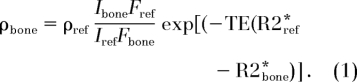Here, ρ_bone and ρ_ref are the water proton densities of bone and reference, respectively. I_bone and I_ref are the image intensities in bone and in the reference, respectively. The factor F represents a fraction of the available magnetization when the duration of the radiofrequency pulse, τ, is comparable to or longer than T2*, TE is echo time, and R2* ≡ 1/T2* is the effective transverse relaxation rate.

Isotope Exchange Experiment

As an independent measurement of BW, the native water in the sheep bone specimens was quantified by immersing the bone in H₂O-D₂O mixtures of varying isotopic composition (0%, 25%, 50%, 75%, and 100% H₂O volume fraction) with approximately 1:25 bone-to-fluid mixture volume ratio for 36 hours at 55°C (to enhance the exchange rate [16]). The time needed for complete exchange was determined in preliminary experiments in which the bone was exposed to increasing periods of immersion in D₂O until the image intensity remained constant. The amount of H₂O in the bone was then calculated by using Equation (2), which is based on the conservation of mass principle that the total amounts of D₂O and H₂O before and after exchange are unaltered:

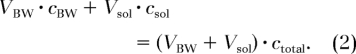Here, V_BW is the BW volume, c_BW is the H₂O concentration of BW before exchange (= 100%), V_sol is the mixture volume, and c_sol and c_total are the H₂O concentrations of the mixture before and after the exchange, respectively. After equilibration, the isotopic ratio of the exchangeable water in the bone and that in the immersion mixture should be equal.

Total water concentration of the human tibia specimens was quantified by immersing the specimens in deuterated water (99.8% deuteration) with an approximate 1:12 volume ratio (bone-to-deuterated water) for 72 hours at 55°C. To minimize any discrepancy between the two measurements that may arise from free water in large macroscopic pores on the endosteal surface, the specimens were blow dried for 2–3 minutes prior to immersion. One milliliter of the mixture was collected before and after the immersion of the bone specimens for MR spectroscopic analysis described below.

Water Quantification at MR Spectroscopy

Quantitative MR spectroscopy was performed with a vertical-bore 9.4-T superconducting spectrometer system (DMX-400; Bruker Instruments, Karlsruhe, Germany) according to the protocol described by Fernandez-Seara et al (22). In brief, the amount of H₂O in the mixture was quantified by recording the integral of the proton signal of the mixture relative to that of a known reference. The MR spectroscopy signal before and after exchange yields the H₂O concentrations c_sol and c_total in Equation (2), from which the total H₂O volume in bone is obtained:

and BW concentration (in percentages by volume) equals (V_BW/V_bone) × 100%, where V_bone is the apparent bone volume, which includes bone tissue and pore volume.

Measurement of BMD

Dual x-ray absorptiometry of the spine and the hip.—Areal BMD (in grams per square centimeter) of the anteroposterior spine and hip were assessed at dual x-ray absorptiometry with a bone densitometer (Hologic; Delphi Systems, Bedford, Mass). Lumbar vertebrae 1 through 4 were measured in the array mode. Spine areal BMD is reported as the average value of the four vertebrae, and hip areal BMD is reported as the average of the left and right hip, each of which is computed as the average of femoral neck, trochanter, and intertrochanteric regions.

Peripheral quantitative CT of the tibia.—Volumetric cortical density, or volumetric BMD (in grams per cubic centimeter), of the tibia was measured by using peripheral quantitative CT (Stratec XCT 2000; Orthometrix, White Plains, NY). First, tibia length was measured from the medial malleolus to the medial tibia condyle by using a segmometer (Rosscraft, Blain, Wash). A scout view was used to identify the medial distal border of the tibia to obtain a tomographic section at the location corresponding to 38% of the tibia length from the distal end (ie, site of maximal cortical thickness) (M.B.L., written communication, January 2008) at a section thickness of 2.3 mm and in-plane pixel size of 0.4 mm. Cortical density (in grams per cubic centimeters) was calculated in the software's research mode by using a threshold-driven mode with filtering, with the threshold set at 711 mg/cm³. Cortical thickness (in millimeters) at this 38% location was also calculated from the studies by using the machine's software.

Statistical Analyses

All statistical analyses were performed with software (JMPIN, version 5.1; SAS Institute, Cary, NC). To evaluate the hypothesized linearity between image-derived water concentration and exchanged water in the validation experiments, the Pearson correlation coefficient was computed. For the in vivo studies, the significance of the mean differences of parameters between patient groups was determined with two-sided t tests. P less than .05 was considered to indicate a significant difference.

RESULTS

Ex Vivo Imaging: Quantification of BW Concentration

Figure 1 shows cross-sectional sheep cortical bone images at five different H₂O concentrations of the H₂O-D₂O immersion mixture. BW signal-to-noise ratio ranged from approximately 45 in its native state (100% H₂O) to approximately 3.5 after complete exchange (nominally 0% H₂O). BW concentration obtained at imaging is plotted in Figure 2 as a function of H₂O concentration in the H₂O-D₂O isotopic mixtures. Measured T1 and T2* at 100% H₂O were 248 msec ± 12 (standard deviation) and 480 μsec ± 22, respectively. The data show that at 100% D₂O there is a small residual signal in bone that is likely to arise from nonexchangeable water or nonwater proton resonances, similar to earlier observations (16). Total BW concentration was found to be 18.5% and 18.8% by volume for specimens A and B, respectively, which is in good agreement with literature data (1,2).

Figure 1:

Transverse ultrashort echo-time MR images of sheep tibia specimens obtained after partial exchange in isotopic mixtures of water, with varying D₂O fractional volume. Percentage values represent H₂O volume fraction, H₂O/(H₂O + D₂O), of the immersion fluid. A = specimen A, B = specimen B.

Figure 2:

Graph of BW concentration quantified from MR images of sheep tibia specimens after graded isotopic exchange with D₂O plotted against fractional H₂O content.

Human Subject Studies

Radial MR images of the human specimens are shown in Figure 3. High-intensity signals arise from periosteum, residual fatty marrow, and inside the endosteal boundary region, presumably due to free water in large pores. T1 and T2* values of the detectable protons in bone were 398 msec ± 7 and 576 μsec ± 38, respectively. Results from imaging and exchange experiments are summarized in Table 1. A paired two-tailed Student t test indicated that measurements from imaging and exchange experiments did not differ significantly from one another (P = .9).

Figure 3a:

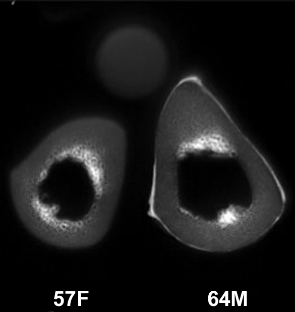
(a–c) Transverse ultrashort echo-time MR images of human specimens of the tibial midshaft from four donors. Specimens of left and right tibia are shown, except in a, where the specimens represent two different donors (57-year-old woman and 64-year-old man). Circular structure superior to specimens is from reference sample. Imaging time was 4 minutes and voxel size was 0.2 × 0.2 × 5 mm.

Figure 3b:

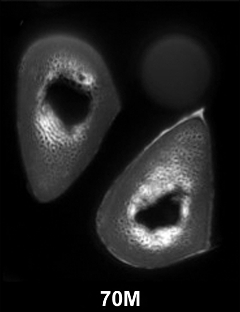
(a–c) Transverse ultrashort echo-time MR images of human specimens of the tibial midshaft from four donors. Specimens of left and right tibia are shown, except in a, where the specimens represent two different donors (57-year-old woman and 64-year-old man). Circular structure superior to specimens is from reference sample. Imaging time was 4 minutes and voxel size was 0.2 × 0.2 × 5 mm.

Figure 3c:

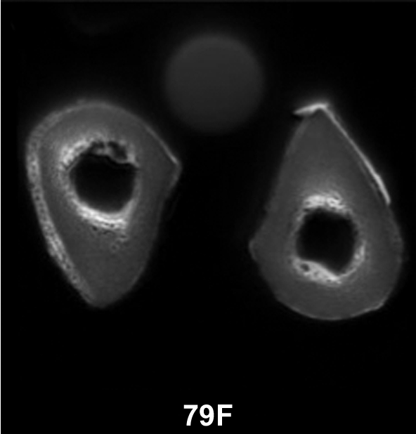
(a–c) Transverse ultrashort echo-time MR images of human specimens of the tibial midshaft from four donors. Specimens of left and right tibia are shown, except in a, where the specimens represent two different donors (57-year-old woman and 64-year-old man). Circular structure superior to specimens is from reference sample. Imaging time was 4 minutes and voxel size was 0.2 × 0.2 × 5 mm.

Table 1.

BW Concentration Measured at Quantitative MR Imaging and Isotope-Exchange MR Spectroscopy in Human Cortical Bone Specimens

Note.—Data are percentages by volume. BW concentrations obtained with the two methods were not significantly different (P = .9).

Transverse images of the tibial midshaft obtained in three subjects (one from each group) are shown in Figure 4. In contrast to the signal void observed with a conventional gradient-echo image (A, D, and G in Figure 4), the ultrashort echo-time radial MR images display elevated signal intensity in solid bone, emphasized with soft-tissue suppression (C, F, and I in Figure 4). BW, BMD, and tibial cortical thickness are listed in Table 2.

Figure 4:

Representative transverse MR images of tibial midshaft from each of the three groups studied, with and without soft-tissue signal suppression. A, D, G, Gradient-echo (GRE) images. B, E, H, Radial ultrashort echo-time images. C, F, I, Radial ultrashort echo-time images with soft-tissue suppression (suppr.). Circular structure is the reference sample with T2 at approximately 300 μsec which, similar to bone, is visible only on radial MR images. Images obtained in 40-year-old healthy subject (top row) display noticeably thicker cortex than in 80-year-old subject (middle row) or in 52-year-old patient with ROD (bottom row). Images in patient with ROD display effect of increased cortical bone porosity.

Table 2.

In Vivo Measurements of Tibial Cortical BW Concentration, Areal BMD of Spine and Hip, and Volumetric BMD and Cortical Thickness of Tibia in Three Groups

Note.—Data are means ± standard deviations.

* Percentage by volume.

BW concentrations were within the range of those found by other investigators by using drying techniques (2,25,26). All BMD values at dual x-ray absorptiometry were in the normal range, except in one subject in the postmenopausal group who had a hip BMD T score less than −2.5. BW concentrations of the pre- and postmenopausal groups were 18.1% ± 2.2 (2D sequence) and 17.4% ± 2.2 (3D sequence) and 30.3% ± 2.0 (2D sequence) and 28.7% ± 1.3 (3D sequence), respectively, and those of the ROD group were 39.5% ± 7.7 (2D sequence) and 41.1% ± 9.6 (3D sequence). No significant difference was found between the 2D and 3D BW measurements with a paired two-tailed Student t test (P = .9, performed with pooled data from all three subject groups).

Figure 5 displays scatterplots of BW and volumetric BMD obtained from the three groups of women. In a comparison among all groups, patients with ROD (intermediate in age between pre- and postmenopausal subjects) had higher BW than the premenopausal group by 135% (P < .001) and than the postmenopausal group by 43% (P = .02). These effects were paralleled by differences of much smaller magnitude (and opposite behavior) in BMD. For example, hip areal BMD was higher by 38% in the premenopausal than in the postmenopausal group (P < .002), whereas volumetric BMD measured at the same tibial site as the BW measurement differed by only 6% between the pre- and postmenopausal groups (P < .003); measurements in patients with ROD did not differ significantly in volumetric BMD from those of either age group of healthy subjects. Cortical thickness was lower in the postmenopausal group by 25% (P < .05) and in the ROD group by 28% (P < .01), compared with the premenopausal group, but cortical thickness was not significantly different between the older and the ROD group. The lack of bone densitometry to differentiate some of the groups may, of course, be due to the study's limited power.

Figure 5a:

Scatterplots show differences between groups for (a) BW and (b) volumetric BMD (vBMD). Data indicate lower BW and higher volumetric BMD in the younger age group. Note abnormally high BW concentration in patients with ROD.

Figure 5b:

Scatterplots show differences between groups for (a) BW and (b) volumetric BMD (vBMD). Data indicate lower BW and higher volumetric BMD in the younger age group. Note abnormally high BW concentration in patients with ROD.

DISCUSSION

Results of this work demonstrate that BW and, by inference, cortical porosity (because the majority of BW is in the spaces of the haversian and lacunocanalicular systems), can be measured noninvasively in patients by using quantitative ultrashort echo-time MR imaging. Most structural imaging of bone has focused on trabecular bone, which remodels faster than cortical bone and therefore responds more quickly to drug intervention. While most osteoporotic fractures occur at sites rich in trabecular bone such as the distal radius, vertebrae, and ribs, the most traumatic fractures are those of the femoral neck, which is characterized by a relatively thick cortex that is known to become porous with advancing age, and more so, in osteoporosis (27).

The results of our pilot study suggest BW to be a more sensitive patient group differentiator than volumetric bone density. For example, BW concentration in the postmenopausal group was 65% larger than that in the premenopausal group (P < .001). In contrast, volumetric density, measured at the same site, was only 6% lower in postmenopausal women. Particularly dramatic is the large increase of BW in patients with ROD, whose cortical BW concentration was 135% higher than that of the premenopausal group (P < .001) and 43% higher than that of the postmenopausal reference group (P = .02). Hence, even though the subject numbers in this pilot study were small, highly significant group differences in BW were observed.

While BMD has been shown to decrease with increasing age (10,28,29), less is known about the changes in BW with age. Results of a few reports involving measurements in cadaveric bone by using destructive techniques suggest that BW increases with age (8,26). Yeni et al (26) found that the age-related decrease in fracture toughness correlated with a decrease in apparent density, which in turn was paralleled by an increase in water concentration and porosity. The authors therefore suggested that the water in the cavities of the bone could be considered “an indicator of porosity.”

Apparent BMD (ie, BMD either areal or volumetric, measured at dual x-ray absorptiometry or at quantitative CT, respectively) is a function of both the amount of bone tissue contained in the total (ie, “apparent”) bone volume, which is the sum of bone tissue and pore volume, and its degree of mineralization of bone (defined as mineral per unit volume of bone tissue, also referred to as the true mineral density). Degree of mineralization of bone can only be measured ex vivo by using microradiography (30) or backscattered electron imaging (31). During the bone-formation process, mineral is deposited onto the osteoid, replacing the space previously occupied by water, therefore leading to the reciprocal relationship of the two constituents (1). This relationship has been observed by Fernandez-Seara et al (22) in osteomalacic rabbits where bone tissue volume was preserved but the tissue was undermineralized (low degree of mineralization of bone).

More commonly, however, bone tissue remains normally mineralized while becoming more porous (eg, secondary to aging) (26,32). This effect leads to a lower amount of bone tissue per unit of overall apparent bone volume; thus, BMD decreases even though degree of mineralization of bone remains unaltered. Because the microscopic pores are filled with water, the lower BMD is associated with higher BW. In ROD, results of recent work (33) in rats suggest the bone to be characterized by extreme porosity. Similarly, the presence of intracortical signal intensity even on conventional spin-echo images in patients receiving maintenance dialysis (23) suggests the bone in chronic kidney disease to be abnormally porous as found in the present work.

Measurement of BW concentration, even ex vivo, is difficult and in the small body of data in the literature, investigators have relied entirely on measuring the weight change upon drying of the bone (2). In the present work, we have validated the imaging-based measurements with a deuterium isotope–exchange technique that involves exchange of native BW with deuterium oxide, followed by proton spectroscopic evaluation of the displaced light water (16). High linearity was achieved between the radial image signal intensity and exchanged water (r² = 0.99, P < .001).

In summary, our data suggest that BW concentration, and thus potentially porosity, can be measured in vivo. The method does not require resolution of individual pores (which are below the resolution limit of all current in vivo imaging modalities); rather, it quantifies pore water on the basis of its unique MR properties. It is therefore not sensitive to partial volume effects and can be practiced at relatively low spatial resolution as long as boundary pixels are excluded from the analysis. A small fraction of the signal cannot be attributed to exchangeable BW as indicated by the residual signal after full exchange was attained. The origin of this residual signal is not known currently and requires further investigation. At present, it can only be concluded that these protons are in a motional environment fast enough to yield a detectable signal at the echo times at which the experiments were conducted. This excludes collagen backbone protons, which have transverse relaxation times less than 20 μsec (34) and would therefore be undetectable. (See also reference 22 and references cited.) Other potential candidates include collagen-bound water in the interior of the collagen's triple helix (3) or mobile side chains of protein constituents with sufficient segmental motion to yield effective transverse relaxation times on the order of 100 μsec or longer. Thus, even though a small portion of the overall signal measured at radial MR imaging is not due to exchangeable water, we still included it in our BW calculation; hence, we are likely to have slightly overestimated the total BW concentration. The concentration of these as of yet unidentified protons is likely to scale with matrix volume (ie, its relative fraction would decrease with decreasing matrix volume).

BW concentrations of the human specimens measured with MR imaging and exchange were not significantly different. However, T1 of the human specimens was longer than those of the sheep specimens (400 vs 250 msec). We attribute the difference to the greater porosity of the human specimens from the relatively old donors (subject age at death, 67 years ± 9), which resulted in greater mobility of water molecules. Water in smaller pores (in younger bone) possesses shorter T1 than that in larger pores (in older bone) because smaller pores have larger surface-to-volume ratio, therefore being more affected by surface relaxivity (35). T2*, on the other hand, seems to be relatively constant. We hypothesize that, unlike at very low field strength, the T2* mechanism of BW at 3.0 T is primarily dictated by susceptibility gradients created at the bone-and-water interface because bone is more diamagnetic than water by about 2.5 ppm (in Système International units) (12). Support for such a mechanism is provided by the field strength dependence of T2*. At 1.5 T, Reichert et al reported T2* of 420–500 μsec in the tibia (36), whereas at 9.4 T, line width-derived measurements in rabbit cortical bone of the femur yielded values of about 200 μsec (37).

There are a number of potential complications with in vivo quantification of BW. While the use of an external reference sample is practical for measurements at relatively superficial locations such as the distal tibia because the radiofrequency field does not vary appreciably across the imaging volume, such an approach is more difficult to realize at deep-lying locations such as the femoral neck. First, radiofrequency inhomogeneity (resulting, for example, from standing wave effects) and depth-dependent receive-coil sensitivity would require more extensive calibration. Alternatively, a reference signal could be derived from adjoining muscle tissue, serving as an internal standard, which then could be calibrated against a reference of known composition. Another potential difficulty is the sensitivity of the derived BW concentration on the relaxation parameters. As pointed out, T2* appears to be relatively invariant whereas T1 can be elongated for highly porous bone, which would therefore necessitate measurement on an individual basis. For reasons not currently understood, T1 of BW is far shorter than that of most soft-tissue water. Therefore, a rapid T1 mapping technique could be appended without significantly prolonging the imaging protocol.

Last, while the initial results reported here are promising, more extensive evaluation will be needed in larger patient studies and in other anatomic sites such as the femoral neck to determine the method's clinical potential. Questions of particular clinical interest are whether BW concentration will be associated with fracture risk and whether this parameter is modifiable with drug intervention, such as antiresorptive or anabolic treatment.

Practical applications: The results of our method for quantifying BW in specimens and in live human subjects suggest that ultrashort echo-time MR imaging may allow routine quantification of cortical bone porosity as a new metric of bone quality in patients with metabolic bone disease.

APPENDIX

In a regime where the duration of the radiofrequency pulse, τ, is comparable to or longer than T2, the simple Bloch equation solutions for the transverse magnetization that assume negligible relaxation during the radiofrequency pulse are no longer valid (see, for example, reference 20) in that a radiofrequency pulse nutates only a fraction of the available magnetization (M_xy(0⁺) < M_z(0⁻)sinα, while for the residual longitudinal magnetization M_z(0⁺) > M_z(0⁻)cosα) holds, where α is the nominal flip angle. Hence, the signal at echo time can be written as:

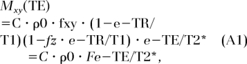where C is a constant and ρ₀ is the proton concentration. The quantities f_z and f_xy are functions of the ratio (τ/T2*), TR is repetition time, and α = γΒ₁τ, given as (21,38):

and

It is readily seen that in the limit where τ is much less than T2*, the quantities f_z and f_xy revert to cosα and sinα. We then obtain the proton concentration in bone, ρ_bone, as:

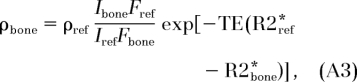where I_bone and I_ref are image intensities of the bone and the reference, respectively. The quantity ρ_ref is the known proton concentration of the reference and R2* ≡ 1/T2*.

Advances in Knowledge.

• A new method is introduced for image-based quantification of cortical bone water (BW) based on ultrashort echo-time radial MR imaging in vivo in human subjects.

• The new method has been validated rigorously and its accuracy demonstrated by means of H₂O-D₂O isotope exchange.

• The measurement of BW constitutes a surrogate parameter for bone porosity that cannot be measured noninvasively with other techniques.

Implications for Patient Care.

• BW concentration constitutes a new parameter for characterizing bone quality.

• Pilot data suggest BW to be a more sensitive discriminator than bone mineral density.

• The method can be implemented with most modern MR imagers.

References

- 1.Elliott SR, Robinson RA.The water content of bone. I. The mass of water, inorganic crystals, organic matrix, and CO2 space components in a unit volume of the dog bone. J Bone Joint Surg Am 1957;39-A:167–188 [PubMed] [Google Scholar]
- 2.Mueller KH, Trias A, Ray RD.Bone density and composition: age-related and pathological changes in water and mineral content. J Bone Joint Surg Am 1966;48:140–148 [PubMed] [Google Scholar]
- 3.Timmins PA, Wall JC.Bone water. Calcif Tissue Res 1977;23:1–5 [DOI] [PubMed] [Google Scholar]
- 4.Garner E, Lakes R, Lee T, Swan C, Brand R.Viscoelastic dissipation in compact bone: implications for stress-induced fluid flow in bone. J Biomech Eng 2000;122:166–172 [DOI] [PubMed] [Google Scholar]
- 5.Laval-Jeantet AM, Bergot C, Carroll R, Garcia-Schaefer F.Cortical bone senescence and mineral bone density of the humerus. Calcif Tissue Int 1983;35:268–272 [DOI] [PubMed] [Google Scholar]
- 6.McCalden RW, McGeough JA, Barker MB, Court-Brown CM.Age-related changes in the tensile properties of cortical bone: the relative importance of changes in porosity, mineralization, and microstructure. J Bone Joint Surg Am 1993;75:1193–1205 [DOI] [PubMed] [Google Scholar]
- 7.Parfitt A.The composition, structure and remodeling of bone: a basis for the interpretation of bone mineral measurements. In Dequeker J, Geusens P, Wahner HW, eds. Bone mineral measurements by photon absorptiometry: methodology problems. Leuven, Belgium: Leuven University Press, 1988 [Google Scholar]
- 8.Nyman JS, Roy A, Tyler JH, Acuna RL, Gayle HJ, Wang X.Age-related factors affecting the postyield energy dissipation of human cortical bone. J Orthop Res 2007;25:646–655 [DOI] [PMC free article] [PubMed] [Google Scholar]
- 9.Basillais A, Bensamoun S, Chappard C, et al. Three-dimensional characterization of cortical bone microstructure by microcomputed tomography: validation with ultrasonic and microscopic measurements. J Orthop Sci 2007;12:141–148 [DOI] [PubMed] [Google Scholar]
- 10.Bousson V, Bergot C, Meunier A, et al. CT of the middiaphyseal femur: cortical bone mineral density and relation to porosity. Radiology 2000;217:179–187 [DOI] [PubMed] [Google Scholar]
- 11.Primer on the metabolic bone diseases and disorders of mineral metabolism. Philadelphia, Pa: Lippincott Williams & Wilkins, 1999 [Google Scholar]
- 12.Hopkins JA, Wehrli FW.Magnetic susceptibility measurement of insoluble solids by NMR: magnetic susceptibility of bone. Magn Reson Med 1997;37:494–500 [DOI] [PubMed] [Google Scholar]
- 13.Robson MD, Gatehouse PD, Bydder M, Bydder GM.Magnetic resonance: an introduction to ultrashort TE (UTE) imaging. J Comput Assist Tomogr 2003;27:825–846 [DOI] [PubMed] [Google Scholar]
- 14.Techawiboonwong A, Song HK, Wehrli FW.In vivo MRI of submillisecond T(2) species with two-dimensional and three-dimensional radial sequences and applications to the measurement of cortical bone water. NMR Biomed 2008;21:59–70 [DOI] [PubMed] [Google Scholar]
- 15.Wu Y, Chesler DA, Glimcher MJ, et al. Multinuclear solid-state three-dimensional MRI of bone and synthetic calcium phosphates. Proc Natl Acad Sci U S A 1999;96:1574–1578 [DOI] [PMC free article] [PubMed] [Google Scholar]
- 16.Fernandez-Seara MA, Wehrli SL, Wehrli FW.Diffusion of exchangeable water in cortical bone studied by nuclear magnetic resonance. Biophys J 2002;82:522–529 [DOI] [PMC free article] [PubMed] [Google Scholar]
- 17.Cooper RR, Milgram JW, Robinson RA.Morphology of the osteon: an electron microscopic study. J Bone Joint Surg Am 1966;48:1239–1271 [PubMed] [Google Scholar]
- 18.Pauly JM, Conolly S, Nishimura D, Macovski A, 28 Slice-selective excitation for very short T2 species [abstr]. In: Book of abstracts: Society of Magnetic Resonance in Medicine 1989. Berkeley, Calif: Society of Magnetic Resonance in Medicine, 1989; 28 [Google Scholar]
- 19.Song HK, Wehrli FW.Variable TE gradient and spin echo sequences for in vivo MR microscopy of short T2 species. Magn Reson Med 1998;39:251–258 [DOI] [PubMed] [Google Scholar]
- 20.Pauly JM, Conolly S, Macovski A.Suppression of long-T2 components for short-T2 imaging [abstr]. In: Book of abstracts: Society for Magnetic Resonance Imaging, 1992; 330. [Google Scholar]
- 21.Sussman MS, Pauly JM, Wright GA.Design of practical T2-selective RF excitation (TELEX) pulses. Magn Reson Med 1998;40:890–899 [DOI] [PubMed] [Google Scholar]
- 22.Fernandez-Seara MA, Wehrli SL, Takahashi M, Wehrli FW.Water content measured by proton-deuteron exchange NMR predicts bone mineral density and mechanical properties. J Bone Miner Res 2004;19:289–296 [DOI] [PubMed] [Google Scholar]
- 23.Wehrli FW, Leonard MB, Saha PK, Gomberg BG.Quantitative high-resolution MRI reveals structural implications of renal osteodystrophy on trabecular and cortical bone. J Magn Reson Imaging 2004;20:83–89 [DOI] [PubMed] [Google Scholar]
- 24.O'Sullivan JD.A fast sinc function gridding algorithm for Fourier inversion in computer tomography. IEEE Trans Med Imaging 1985;4:200–207 [DOI] [PubMed] [Google Scholar]
- 25.Biltz RM, Pellegrino ED.The chemical anatomy of bone. I. A comparative study of bone composition in sixteen vertebrates. J Bone Joint Surg Am 1969;51:456–466 [PubMed] [Google Scholar]
- 26.Yeni YN, Brown CU, Norman TL.Influence of bone composition and apparent density on fracture toughness of the human femur and tibia. Bone 1998;22:79–84 [DOI] [PubMed] [Google Scholar]
- 27.Bell KL, Loveridge N, Jordan GR, Power J, Constant CR, Reeve J.A novel mechanism for induction of increased cortical porosity in cases of intracapsular hip fracture. Bone 2000;27:297–304 [DOI] [PubMed] [Google Scholar]
- 28.Tanno M, Horiuchi T, Nakajima I, Maeda S, Igarashi M, Yamada H.Age-related changes in cortical and trabecular bone mineral status: a quantitative CT study in lumbar vertebrae. Acta Radiol 2001;42:15–19 [DOI] [PubMed] [Google Scholar]
- 29.Russo CR, Lauretani F, Bandinelli S, et al. Aging bone in men and women: beyond changes in bone mineral density. Osteoporos Int 2003;14:531–538 [DOI] [PubMed] [Google Scholar]
- 30.Meunier PJ, Boivin G.Bone mineral density reflects bone mass but also the degree of mineralization of bone: therapeutic implications. Bone 1997;21:373–377 [DOI] [PubMed] [Google Scholar]
- 31.Boyde A, Jones SJ, Aerssens J, Dequeker J.Mineral density quantitation of the human cortical iliac crest by backscattered electron image analysis: variations with age, sex, and degree of osteoarthritis. Bone 1995;16:619–627 [DOI] [PubMed] [Google Scholar]
- 32.Bousson V, Peyrin F, Bergot C, Hausard M, Sautet A, Laredo JD.Cortical bone in the human femoral neck: three-dimensional appearance and porosity using synchrotron radiation. J Bone Miner Res 2004;19:794–801 [DOI] [PubMed] [Google Scholar]
- 33.Hopper TA, Wehrli FW, Saha PK, et al. Quantitative microcomputed tomography assessment of intratrabecular, intertrabecular, and cortical bone architecture in a rat model of severe renal osteodystrophy. J Comput Assist Tomogr 2007;31:320–328 [DOI] [PubMed] [Google Scholar]
- 34.Edzes HT, Samulski ET.Cross relaxation and spin diffusion in the proton NMR or hydrated collagen. Nature 1977;265:521–523 [DOI] [PubMed] [Google Scholar]
- 35.Ni Q, King J, Wang X.The characterization of human compact bone structure changes by low-field nuclear magnetic resonance. Meas Sci Technol 2004;15:58–66 [Google Scholar]
- 36.Reichert IL, Robson MD, Gatehouse PD, et al. Magnetic resonance imaging of cortical bone with ultrashort TE pulse sequences. Magn Reson Imaging 2005;23:611–618 [DOI] [PubMed] [Google Scholar]
- 37.Anumula S, Magland J, Wehrli S, Ong H, Song H, Wehrli FW.Multi-modality study of the compositional and mechanical implications of hypomineralization in a rabbit model of osteomalacia. Bone 2008;42:405–413 [DOI] [PMC free article] [PubMed] [Google Scholar]
- 38.Hu BS, Conolly SM, Wright GA, Nishimura DG, Macovski A.Pulsed saturation transfer contrast. Magn Reson Med 1992;26:231–240 [DOI] [PubMed] [Google Scholar]