Model-Based Segmentation of Hippocampal Subfields in Ultra-High Resolution In Vivo MRI

Abstract

Recent developments in MR data acquisition technology are starting to yield images that show anatomical features of the hippocampal formation at an unprecedented level of detail, providing the basis for hippocampal subfield measurement. Because of the role of the hippocampus in human memory and its implication in a variety of disorders and conditions, the ability to reliably and efficiently quantify its subfields through in vivo neuroimaging is of great interest to both basic neuroscience and clinical research. In this paper, we propose a fully-automated method for segmenting the hippocampal subfields in ultra-high resolution MRI data. Using a Bayesian approach, we build a computational model of how images around the hippocampal area are generated, and use this model to obtain automated segmentations. We validate the proposed technique by comparing our segmentation results with corresponding manual delineations in ultra-high resolution MRI scans of five individuals.

1 Introduction

Models of brain structures generated from magnetic resonance imaging (MRI) data have grown in complexity in recent years, evolving from simple models with few classes such as gray matter, white matter and cerebrospinal fluid (CSF) [1,2,3], into more complex ones representing a multitude of neuroanatomical structures [4,5,6]. Still, while many brain structures such as the thalamus, the amygdala, or the hippocampus consist of multiple distinct, interacting subregions, they are mostly treated as a single entity because of the limited image resolution of typical structural MRI scans. Recently, however, substantial developments in MR data acquisition technology have made it possible to acquire images with remarkably higher resolution and signal-to-noise ratio than was previously attainable [7]. Such scans show many cortical and subcortical structures in unprecedented detail, and offer new opportunities for explicitly quantifying individual subregions, rather than their agglomerate, directly from in vivo MRI data.

Analyzing large imaging studies of ultra-high resolution MRI scans requires computational techniques to automatically extract information from the images. This is technically difficult because, although the images show greater anatomical detail than traditional MRI scans, many boundaries between substructures of interest remain hard to discern. In manual delineations, the extent of specific subregions is often inferred from the extent of other, more clearly defined structures by relying on prior neuroanatomical knowledge, rather than on local intensity information alone. The success of automated methods therefore depends critically on computational models that provide prior information about the relative location, shape, and appearance of the structures of interest.

In this paper, we present an automated segmentation technique for the subfields of the hippocampus in ultra-high resolution MRI data based on state-of-the-art computational models. Although the methodology is applicable to other brain structures as well, we identified the hippocampus as our driving application because it is a necessary component in a variety of memory functions, as well as the locus of structural change in aging, Alzheimer's disease (AD), schizophrenia, and other conditions. Distinct hippocampal subregions have been shown to be implicated in different memory subsystems [8,9] and be differentially affected in aging and AD [10]. Therefore, the ability to measure, through in vivo neuroimaging, subtle changes in these subregions promises to have widespread application in both basic neuroscience and clinical research.

2 Model-Based Hippocampal Subfield Segmentation

We use a Bayesian modeling approach, in which we first build an explicit computational model of how an MRI image around the hippocampal area is generated, and subsequently use this model to obtain fully automated segmentations. The model incorporates a prior distribution that makes predictions about where neuroanatomical labels typically occur throughout the image, and is based on the generalization of probabilistic atlases [2,3,4,5,11] developed in [12]. The model also includes a likelihood distribution that predicts how a label image, where each voxel is assigned a unique neuroanatomical label, translates into an MRI image, where each voxel has an intensity.

2.1 Prior: Mesh-Based Probabilistic Atlas

Let L = {l_i,i = 1,...,} be a label image with a total of I voxels, with l_{i∈ {}1,...,K} denoting the one of K possible labels assigned to voxel i. Our prior models this image as being generated by the following process:

• A (irregular) tetrahedrical mesh covering the image domain of interest is defined by the reference position of its N mesh nodes ${\mathit{x}}^r=\{{\mathit{x}}_n^r,n=1,\dots ,N\}$, and by a set of label probabilities α = {α_n, n = 1,...,N}. Node n is associated with a probability vector ${\alpha }_n=\{{\alpha }_n^1,\dots ,{\alpha }_n^K\}$, satisfying ${\alpha }_n^k\ge 0$ and ${\sum }_k^K{\alpha }_n^k=1$, that governs how frequently each label occurs around that node.

• The mesh is deformed from its reference position by sampling from a Markov random field (MRF) model regulating the position of the mesh nodes:

  $$p\left(x\right)\propto \text{exp}\left(-U_{x^r}\left(x\right)\right)=\text{exp}\left(-\sum _{t=1}^T{U}_{x^r}^t\left(x\right)\right),$$ (1)

  where $U_{{\mathit{x}}^r}^t\left(\mathit{x}\right)$ is a penalty for deforming tetrahedron t from its shape in the reference position x^r, and U_x^r (x) is an overall deformation penalty obtained by summing the contributions of all T tetrahedra in the mesh. We use the penalty proposed in [13], which goes to infinity if the Jacobian determinant of any tetrahedron's deformation approaches zero, and therefore insures that the mesh topology is preserved.
• In the deformed mesh with position x, the probability of observing label k in a pixel i with location x_i is modeled by

  $$p_i(k\mid x)=\sum _{n=1}^N{\alpha }_n^k{\varphi }_n\left(x_i\right),$$ (2)

  where φ_n(·) denotes an interpolation basis function attached to mesh node n that has a unity value at the position of the mesh node, a zero value at the outward faces of the tetrahedra connected to the node and beyond, and a linear variation across the volume of each tetrahedron. Assuming conditional independence of the labels between voxels given the mesh node locations, we obtain the probability of seeing label image $L:p(L\mid \mathit{x})={\prod }_{i=1}^I{p}_i(l_i\mid \mathit{x})$.

It has previously been demonstrated that the mesh's connectivity, reference position x^r, and label probabilities α can be learned from a set of manually labeled example images [12]. The learning involves selecting the model that maximizes the probability of observing the example label images, or, equivalently, that minimizes the number of bits needed to encode them. An example of the prior, derived from 4 manually labeled hippocampi, is shown in figure 2. Note that the image domain is non-uniformly sampled, with areas containing little information covered by larger tetrahedra.

Fig. 2.

Mesh-based probabilistic atlas, derived from manual delineations in 4 subjects, warped onto the 5th subject shown in figure 1. Bright and dark intensities correspond to high and low prior probability for subiculum, respectively.

2.2 Likelihood: Imaging Model

For the likelihood distribution, we employ a simple, often-used model according to which a Gaussian distribution with mean μ_k and variance ${\sigma }_k^2$ is associated with each label k. Given label image L, an intensity image Y = {y_i, i = 1,...,I} is generated by drawing the intensity in each voxel independently from the Gaussian distribution associated with its label:

$$p(Y\mid L,\theta )=\prod _{i=1}^{I}p(y_i\mid {\mu }_{l_i},{\sigma }_{l_i}^2)=\prod _{i=1}^I\frac{1}{\sqrt{2\pi {\sigma }_{l_i}^2}}\text{exp}\left(-\frac{{(y_i-{\mu }_{l_i})}^2}{2{\sigma }_{l_i}^2}\right),$$

where the parameters $\theta =\{{\mu }_1,{\sigma }_1^2,\dots ,{\mu }_K,{\sigma }_K^2\}$ are assumed to be governed by a uniform prior: p(θ) ∝ 1.

2.3 Model Parameter Estimation

In a Bayesian setting, assessing the Maximum A Posteriori (MAP) parameter values $\{\widehat{\mathit{x}},\widehat{\theta }\}$ involves maximizing

$$p(x,\theta \mid Y)\propto p(Y\mid x,\theta )p\left(x\right)p\left(\theta \right)\propto \left(\prod _{i=1}^I\sum _{k=1}^{K}p(y_i\mid {\mu }_k,{\sigma }_k^2)p_i(k\mid x)\right)p\left(x\right),$$

which is equivalent to minimizing

$$\sum _{i=1}^I\left(-\text{log}\left[\sum _{k=1}^{K}p(y_i\mid {\mu }_k,{\sigma }_k^2)p_i(k\mid x)\right]\right)-\text{log}p\left(x\right).$$ (3)

We use an EM-style majorization technique [14,15], where we calculate a statistical classification that associates each voxel with each of the neuroanatomical labels

$$W_i^k=\frac{p(y_i\mid {\mu }_k,{\sigma }_k^2)p_i(k\mid x)}{{\Sigma }_{k^{\prime }}p(y_i\mid {\mu }_{k^{\prime }},{\sigma }_{k^{\prime }}^2)p_i(k^{\prime }\mid x)}$$

and subsequently use this classification to construct an upper bound to eq. (3) that touches it at the current parameters estimates [16]:

$$\sum _{i=1}^I\left(-\text{log}\left[\prod _{k=1}^K{\left(\frac{p(y_i\mid {\mu }_k,{\sigma }_k^2)p_i(k\mid x)}{W_i^k}\right)}^{W_i^k}\right]\right)-\text{log}p\left(x\right).$$ (4)

Optimizing this upper bound w.r.t. the Gaussian distribution parameters θ, while keeping x fixed, yields the closed-form expressions

$${\mu }_k=\frac{\sum _{i=1}^I{W}_i^k{y}_i}{\sum _{i=1}^I{W}_i^k},{\sigma }_k^2=\frac{\sum _{i=1}^I{W}_i^k{(y_i-{\mu }_k)}^2}{\sum _{i=1}^I{W}_i^k},k=1,\dots ,K.$$

With these estimates of θ, the classification and the corresponding upper bound are updated, and the estimation of θ is repeated, until convergence. We then re-calculate the upper bound, and optimize it w.r.t. the mesh node positions x, keeping θ fixed. Optimizing x is a registration process that deforms the atlas mesh towards the current classification, similar to the schemes proposed in [5,17]. The gradient of eq. (4) with respect to x is given in analytical form through the interpolation model of eq. (2) and the deformation model of eq. (1). We perform this registration by gradient descent. Subsequently, we repeat the optimization of θ and x, each in turn, until convergence.

2.4 Image Segmentation

Once we have an estimate of the model parameters $\{\widehat{\mathit{x}},\widehat{\theta }\}$, we can use it to obtain an approximation to the MAP anatomical labeling. Approximating $p(L\mid Y)={\int }_{\mathit{x}}{\int }_{\theta }p(L\mid Y,\mathit{x},\theta )p(\mathit{x},\theta \mid Y)\mathrm{d}\mathit{x}\mathrm{d}\theta \text{by}p(L\mid Y,\widehat{\mathit{x}},\widehat{\theta })\propto p(Y\mid L,\widehat{\theta })p(L\mid \widehat{\mathit{x}})$, we have

$$\widehat{L}=\text{arg}\underset{L}{\text{max}}p(L\mid Y)\simeq \text{arg}\underset{\{l_i,i=1,\dots ,I\}}{\text{max}}\prod _i^{I}p(y_i\mid {\widehat{\mu }}_{l_i},{\widehat{\sigma }}_{l_i}^2)p_i(l_i\mid \widehat{x}),$$

which is obtained by assigning each voxel to the label with the highest posterior probability, i.e., ${\widehat{l}}_i=\arg {\max }_k{W}_i^k$.

3 Experiments

We performed experiments on ultra-high resolution MRI data collected as part of an ongoing imaging study assessing the effects of normal aging and AD on brain structure. Using a prototype custom-built 32-channel head coil with a 3.0T Siemens Trio MRI system [7], we acquired images via an optimized high-resolution MPRAGE sequence that enables 380 μm in-plane resolution (TR/TI/TE = 2530/1100/5.39 ms, FOV=448, FA = 7°, 208 slices acquired coronally, thickness = 0.8mm, acquisition time = 7.34 min). To increase the signal-to-noise ratio, 5 acquisitions were collected and motion-corrected to obtain a single resampled (to 380 μm isotropic) high contrast volume that covers the entire medial temporal lobe.

Using a protocol developed specifically for this purpose, the subfields of the right hippocampus were manually delineated in images of 5 subjects (2 younger and 3 older cognitively normal individuals). These delineations included the fimbria, presubiculum, subiculum, CA1, CA2/3, and CA4/DG fields, as well as choroid plexus, hippocampal fissure, and lateral ventricle, as shown in figure 1. Voxels outside of these structures were automatically labeled as gray matter, white matter, or CSF using an EM-based tissue classifier [2].

Fig. 1.

From left to right: ultra-high resolution MRI data, manual delineations, and corresponding automated segmentations

We restricted our automated analysis to a region of interest (ROI) around the right hippocampus only. To this end, we defined a cuboid ROI of size 100×60×160 voxels in an image of a younger normal individual not included in the study (template image). This ROI was automatically aligned to each image under study using an affine Mutual Information based registration technique [18,19], by first aligning the whole template image covering the entire brain, followed by a registration of the ROI only. Atlas meshes were then computed and applied in the area covered by this ROI in each image.

We used a 3-level multi-resolution optimization strategy, in which the image under study and the atlas mesh were subject to a gradually decreasing amount of spatial smoothing. In order to simplify the optimization process, we restricted the number of labels throughout the multi-resolution scheme to four, merging the gray matter with the presubiculum, subiculum, and CA fields, the white matter with the fimbria, the lateral ventricle with choroid plexus, and CSF with the hippocampal fissure. This restriction was then removed to obtain the final segmentation. The whole segmentation process was fully automated and took about 1.5 hours per subject on a 2.33GHz Intel Core2 processor.

We evaluated our automated segmentation results using a leave-one-out cross-validation strategy: we built an atlas mesh from the delineations in 4 subjects, and used this to segment the image of the remaining subject. We repeated this process for each of the 5 subjects, and compared the automated segmentation results with the corresponding manual delineations. Towards the tail of the hippocampus, the manual delineations no longer discerned between the different subfields, but rather lumped everything together as simply “hippocampus” (see figure 1). Since the starting point of this “catch-all” label was arbitrary chosen in each subject, with its volume ranging from 5 to 17% of the total hippocampal volume in different subjects, voxels that were labeled as such in either the automated or manual segmentation were not included in the comparisons.

For each of seven structures of interest (fimbria, CA1, CA2/3, CA4/DG, presubiculum, subiculum, and hippocampal fissure), we calculated the Dice overlap coefficient, defined as the volume of overlap between the automated and manual segmentation divided by their mean volume. Since we are ultimately interested in detecting changes in hippocampal subfields between different patient populations, we also evaluated how well differences in subfield volumes between subjects, as detected by the manual delineations, were reflected in the automated segmentations. To this end, we performed a linear regression on the absolute volumes detected by both methods, calculating Pearson's correlation coefficient for each structure.

4 Results

Figure 1 compares the manual and automated segmentation results qualitatively on a set of cross-sectional slices. The upper half of figure 3 shows the average Dice overlap measure for each of the structures of interest, along with the minimum and maximum across the 5 subjects. All of the larger structures, ranging in average size from 6,100 voxels for CA1 to 14,300 voxels for CA2/3, have an average Dice coefficient of around 0.7 or higher. Smaller structures such as the fimbria (on average 1,700 voxels) and the hippocampal fissure (on average 1,400 voxels) are more challenging and have a lower Dice coefficient of around 0.58 and 0.45, respectively.

Fig. 3.

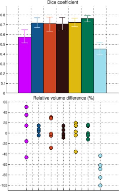
Dice overlap measures (top) and relative volume differences (bottom) between automated and manual segmentations. The colors are as in figure 1.

The lower half of figure 3 shows, for each structure, the volume differences between the automated and manual segmentations relative to their mean volumes. Regarding Pearson's correlation coefficient, the automatically calculated volumes of CA4/DG and CA2/3 are strongly correlated with the manual ones, with a correlation coefficient of approximately 0.98 (p ≤ 0.004) and 0.93 (p ≤ 0.024), respectively. CA1 and subiculum correlate to some degree (correlation coefficient of 0.73 and 0.71, p-values not significant), whereas presubiculum and fimbria do not seem to correlate at all (correlation coefficient of 0.02 and −0.18, p-values not significant). Interestingly, despite the hippocampal fissure's low Dice overlap measure, its automated measurements correlate better with the manual ones than do some structures with much higher Dice coefficients (correlation coefficient 0.85, p ≤ 0.068). The low Dice coefficient is apparently caused by a systematic underestimation of the hippocampal fissure volume by the automated method.

5 Discussion

In this paper, we demonstrated a model-based approach to automated hippocampal subfield segmentation in ultra-high resolution MRI and presented preliminary results on a small number of subjects. Future work will include a more thorough validation, using more subjects with repeat scans and manual delineations by different raters, so that the accuracy and repeatability of our method can be placed in context. Furthermore, in order to analyze invaluable existing imaging studies that were acquired at more standard image resolutions, we also plan to develop a modified likelihood for standard resolution images that includes an explicit model of the partial volume effect [20].

References

- 1.Wells W, et al. Adaptive segmentation of MRI data. IEEE Transactions on Medical Imaging. 1996;15(4):429–442. doi: 10.1109/42.511747. [DOI] [PubMed] [Google Scholar]
- 2.Van Leemput K, et al. Automated model-based tissue classification of MR images of the brain. IEEE Transactions on Medical Imaging. 1999;18(10):897–908. doi: 10.1109/42.811270. [DOI] [PubMed] [Google Scholar]
- 3.Ashburner J, Friston K. Unified segmentation. NeuroImage. 2005;26:839–885. doi: 10.1016/j.neuroimage.2005.02.018. [DOI] [PubMed] [Google Scholar]
- 4.Fischl B, et al. Whole brain segmentation: Automated labeling of neuroanatomical structures in the human brain. Neuron. 2002;33:341–355. doi: 10.1016/s0896-6273(02)00569-x. [DOI] [PubMed] [Google Scholar]
- 5.Pohl K, et al. A Bayesian model for joint segmentation and registration. NeuroImage. 2006;31:228–239. doi: 10.1016/j.neuroimage.2005.11.044. [DOI] [PubMed] [Google Scholar]
- 6.Heckemann R, et al. Automatic anatomical brain MRI segmentation combining label propagation and decision fusion. NeuroImage. 2006;33(1):115–126. doi: 10.1016/j.neuroimage.2006.05.061. [DOI] [PubMed] [Google Scholar]
- 7.Wiggins G, et al. 32-channel 3 Tesla receive-only phased-array head coil with soccer-ball element geometry. Magn. Res. in Medicine. 2006;56(1):216–223. doi: 10.1002/mrm.20925. [DOI] [PubMed] [Google Scholar]
- 8.Zeineh M, et al. Dynamics of the Hippocampus During Encoding and Retrieval of Face-Name Pairs. Science. 2003;299(5606):577–580. doi: 10.1126/science.1077775. [DOI] [PubMed] [Google Scholar]
- 9.Gabrieli J, et al. Separate Neural Bases of Two Fundamental Memory Processes in the Human Medial Temporal Lobe. Science. 1997;276(5310):264. doi: 10.1126/science.276.5310.264. [DOI] [PubMed] [Google Scholar]
- 10.Small S, et al. Evaluating the function of hippocampal subregions with high-resolution MRI in AD and aging. Microsc. Res. and Tech. 2000;51(1):101–108. doi: 10.1002/1097-0029(20001001)51:1<101::AID-JEMT11>3.0.CO;2-H. [DOI] [PubMed] [Google Scholar]
- 11.Shattuck D, et al. Construction of a 3D probabilistic atlas of human cortical structures. NeuroImage. 2008;39:1064–1080. doi: 10.1016/j.neuroimage.2007.09.031. [DOI] [PMC free article] [PubMed] [Google Scholar]
- 12.Van Leemput K. Probabilistic brain atlas encoding using Bayesian inference. In: Larsen R, Nielsen M, Sporring J, editors. MICCAI 2006. LNCS. Vol. 4190. Springer; Heidelberg: 2006. pp. 704–711. [DOI] [PubMed] [Google Scholar]
- 13.Ashburner, et al. Image registration using a symmetric prior–in three dimensions. Human Brain Mapping. 2000;9(4):212–225. doi: 10.1002/(SICI)1097-0193(200004)9:4<212::AID-HBM3>3.0.CO;2-#. [DOI] [PMC free article] [PubMed] [Google Scholar]
- 14.Dempster AP, et al. Maximum likelihood from incomplete data via the EM algorithm. Journal of the Royal Statistical Society. 1977;39:1–38. [Google Scholar]
- 15.Stoica P, Selén Y. Cyclic minimizers, majorization techniques, and the EM algorithm: A refresher. IEEE Signal Processing Magazine. 2004:112–114. [Google Scholar]
- 16.Minka T. Expectation-Maximization as lower bound maximization. Technical report, MIT. 1998 [Google Scholar]
- 17.D'Agostino E, et al. A unified framework for atlas based brain image segmentation and registration. In: Pluim JPW, Likar B, Gerritsen FA, editors. WBIR 2006. LNCS. Vol. 4057. Springer; Heidelberg: 2006. pp. 136–143. [Google Scholar]
- 18.Wells W, et al. Multi-modal volume registration by maximization of mutual information. Medical Image Analysis. 1996;1(1):35–51. doi: 10.1016/s1361-8415(01)80004-9. [DOI] [PubMed] [Google Scholar]
- 19.Maes F, et al. Multimodality image registration by maximization of mutual information. IEEE Transactions on Medical Imaging. 1997;16(2):187–198. doi: 10.1109/42.563664. [DOI] [PubMed] [Google Scholar]
- 20.Van Leemput K, et al. A unifying framework for partial volume segmentation of brain MR images. IEEE Transactions on Medical Imaging. 2003;22(1):105–119. doi: 10.1109/TMI.2002.806587. [DOI] [PubMed] [Google Scholar]