Decoding and Reconstructing Color from Responses in Human Visual Cortex

Abstract

How is color represented by spatially distributed patterns of activity in visual cortex? Functional magnetic resonance imaging responses to several stimulus colors were analyzed with multivariate techniques: conventional pattern classification, a forward model of idealized color tuning, and principal component analysis (PCA). Stimulus color was accurately decoded from activity in V1, V2, V3, V4, and VO1 but not LO1, LO2, V3A/B, or MT+. The conventional classifier and forward model yielded similar accuracies, but the forward model (unlike the classifier) also reliably reconstructed novel stimulus colors not used to train (specify parameters of) the model. The mean responses, averaged across voxels in each visual area, were not reliably distinguishable for the different stimulus colors. Hence, each stimulus color was associated with a unique spatially distributed pattern of activity, presumably reflecting the color selectivity of cortical neurons. Using PCA, a color space was derived from the covariation, across voxels, in the responses to different colors. In V4 and VO1, the first two principal component scores (main source of variation) of the responses revealed a progression through perceptual color space, with perceptually similar colors evoking the most similar responses. This was not the case for any of the other visual cortical areas, including V1, although decoding was most accurate in V1. This dissociation implies a transformation from the color representation in V1 to reflect perceptual color space in V4 and VO1.

Introduction

Although the early stages of color vision are well understood, the representation of color in visual cortex remains enigmatic. Color vision begins with three types of cone photoreceptors that are recombined into color-opponent channels (Derrington et al., 1984; Kaiser and Boynton, 1996; Gegenfurtner, 2003). Many neurons in visual cortex are color selective (Dow and Gouras, 1973; Solomon and Lennie, 2007), and color-opponent responses are evident throughout visual cortex (Kleinschmidt et al.,1996; Engel et al., 1997). In macaque area V4, the majority of neurons were reported to be chromatically tuned (Zeki, 1974), and, although disputed (Schein et al., 1982), more recent work has revealed patches of inferior temporal cortex (including V4) that respond more strongly to chromatic stimuli than to achromatic stimuli (Conway et al., 2007). Similarly, imaging studies have demonstrated chromatic selectivity in human V4 (Bartels and Zeki, 2000) and in areas anterior to V4 (V8, Hadjikhani et al., 1998; VO1, Brewer et al., 2005). A remaining question, however, is how visual cortex transforms color-opponent signals into the perceptual color space.

This question might be addressed by the application of multivariate analysis methods, such as pattern classification, to functional magnetic resonance imaging data (fMRI). Given that there are color-selective neurons in visual cortex, it may be possible to associate each color with a unique spatial pattern of fMRI responses, although each fMRI voxel shows only a weak tuning to color. This approach has been used successfully to distinguish between objects categories (Haxby et al., 2001), hand gestures (Dinstein et al., 2008), and visual features (Kamitani and Tong, 2005). Advancing these methods, Kay et al. (2008) measured fMRI responses to natural images, modeled the activity in each voxel as a weighted sum of idealized neural responses, and then used the model to identify a novel image based on the pattern of activity that it evoked.

Here, we report that color is represented differently in the spatially distributed patterns of activity in different visual cortical areas. We characterized the distributed response patterns to several colors with three complementary, multivariate analysis techniques: conventional pattern classification, a model of idealized color tuning (“forward model”), and principal component analysis (PCA). Stimulus color was accurately decoded from activity in V1, V2, V3, V4, and VO1 but not LO1, LO2, V3A/B, or MT+. The conventional classifier and forward model yielded similar accuracies, but the forward model also reliably reconstructed novel stimulus colors. The mean responses, averaged across voxels in each visual area, were not reliably distinguishable for the different stimulus colors. Using PCA, a color space was derived from the covariation in the responses to different colors. In V4 and VO1, the first two principal components of the responses revealed a progression through perceptual color space, with perceptually similar colors evoking the most similar responses. This was not found for V1, although decoding was most accurate in V1. This dissociation implies a transformation from the color representation in V1 to reflect perceptual color space in V4 and VO1.

Materials and Methods

Observers and scanning sessions.

Five healthy observers between the ages of 23 and 37 years participated in this study. Observers provided written informed consent. Experimental procedures were in compliance with the safety guidelines for MRI research and were approved by the University Committee on Activities Involving Human Subjects at New York University. Observers had normal or corrected-to-normal vision. Normal color vision was verified by use of the Ishihara plates (Ishihara, 1917) and a computerized version of the Farnsworth–Munsell 100 hue-scoring test (Farnsworth, 1957). Each observer participated in three to five experimental sessions, consisting of 8–10 runs of the main color experiment. Observers also participated in a retinotopic mapping session and a session in which a high-resolution anatomical volume was acquired.

Experimental protocol.

Stimuli were concentric sinusoidal gratings, within a circular aperture modulating between the center gray point and one of eight different locations in color space. The eight colors were equally spaced in Commission Internationale de l'Eclairage (CIE) L*a*b* space, at a fixed lightness of L* = 75 (corresponding to 8.8 cd/m²) and equidistant from the gray point at L* = 75, a* = 0, and b* = 0 (Fig. 1A,B). The CIE L*a*b* space is a nonlinear transform of the CIE xyz color space, intended to be more perceptually uniform (Commission Internationale de l'Eclairage, 1986). The gratings slowly drifted either inward or outward, with the direction chosen randomly for each trial. Visual stimuli appeared for a duration of 1.5 s in a randomized order. Using an event-related design, interstimulus intervals (ISIs) ranged from 3 to 6 s, in steps of 1.5 s (Fig. 1C). All eight colors were presented eight times in each run, along with eight blank trials. This created a total of 72 trials per run, with one run lasting 7 min and 12 s.

Figure 1.

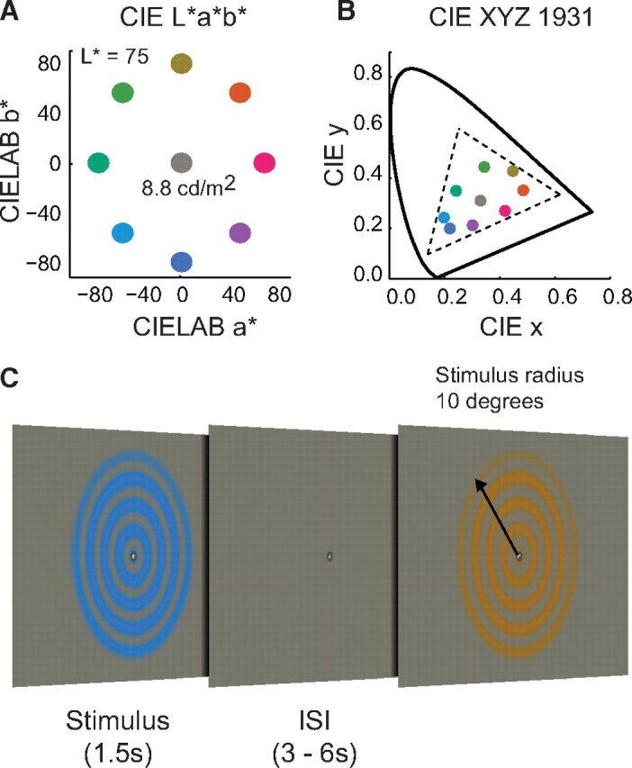
Stimulus and experimental protocol. A, Location of the eight colors and gray point in CIE L*a*b* space. Colors were presented at a lightness of L* = 75 (8.8 cd/m²). B, The same eight colors and gray point in CIE 1931 xyz space. C, Stimuli were concentric sinusoidal gratings (spatial frequency, 0.5 cycles/°), within a circular aperture (10° radius), modulating from a center gray point to one of the eight locations in color space. Stimuli drifted either inward or outward, at a speed of 1°/s. Stimulus duration, 1.5 s. Interstimulus interval, 3–6 s in steps of 1.5 s.

Observers performed a “rapid serial visual presentation” detection task continuously throughout each run, to maintain a consistent behavioral state and to encourage stable fixation. A sequence of characters, randomly colored either black or white, was displayed on the fixation point (each appearing for 400 ms). The observer's task was to detect a specific sequence of characters, pressing a button when a white “K” was followed immediately by a black “K.”

Response time courses and response amplitudes.

fMRI data were preprocessed using standard procedures. The first four images of each run were discarded to allow the longitudinal magnetization to reach steady state. We compensated for head movements within and across runs using a robust motion estimation algorithm (Nestares and Heeger, 2000), divided the time series of each voxel by its mean image intensity to convert to percentage signal change and compensate for distance from the radio frequency coil, and linearly detrended and high-pass filtered the resulting time series with a cutoff frequency of 0.01 Hz to remove low-frequency drift.

The hemodynamic impulse response function (HIRF) of each voxel was estimated with deconvolution (Dale, 1999), averaging across all stimuli (ignoring stimulus color so as to avoid introducing any statistical bias in the decoding accuracies). Specifically, we computed the mean response for 12 s (eight time points) after stimulus presentation, separately for each voxel, using linear regression. In the first column of the regression matrix, 1 was at the onset of stimuli and 0 elsewhere. For each of the 11 remaining columns, we progressively shifted the ones forward one time point. HIRFs were estimated by multiplying the pseudoinverse of this regression matrix with the measured (and pre-processed) fMRI response time courses. This procedure assumed linear temporal summation of the fMRI responses (Boynton et al., 1996; Dale, 1999) but did not assume any particular time course for the HIRFs. The goodness of fit of the regression model, r², was computed as the amount of variance accounted for by the estimated HIRFs (Gardner et al., 2005). That is, the estimated HIRFs computed by deconvolution were convolved with the stimulus times to form a model response time course, and r² was then computed as the amount of variance in the original time course accounted for by this model response time course.

The HIRFs were averaged across the subset of voxels in each visual cortical area that responded strongly to the stimuli. A region of interest (ROI) was defined for each visual area, separately for each observer, using retinotopic mapping procedures (see below). The mean HIRF of each ROI was then computed by averaging the HIRFs of voxels with an r² above the median for that ROI (supplemental Fig. 1, available at www.jneurosci.org as supplemental material).

The response amplitudes to each color were computed separately for each voxel in each ROI and separately for each run, using linear regression. A regression matrix was constructed for each ROI by convolving the ROI-specific HIRF and its numerical derivative with binary time courses corresponding to the onsets of each of the eight stimulus colors (with 1 at each stimulus onset and 0 elsewhere). The resulting regression matrix had 16 columns: eight columns for the HIRF convolved with each of the eight stimulus onsets and eight columns for the HIRF derivative convolved with each of the eight stimulus onsets. Response amplitudes were estimated by multiplying the pseudoinverse of this regression matrix with the measured (and pre-processed) fMRI response time courses. We included the derivative because the HIRF of an individual voxel may have differed from the mean HIRF of the ROI of that voxel. At least some of the response variability was captured by including the derivative; the variance of the estimated response amplitudes across runs was smaller with the derivative included than without it. The values obtained for the derivative regressors were discarded after response amplitudes were estimated. We thus obtained, for each voxel and each run, one response amplitude estimate for each of the eight colors. These response amplitudes were z-score normalized, separately for each voxel, separately for each run.

Combining across sessions and reducing dimensionality.

To increase decoding accuracy, we combined the data from multiple scanning sessions. The estimated response amplitudes from a single visual area ROI in a single session formed an m × n matrix, with m being the number of voxels in the ROI (or dimensions) and n being the number of repeated measurements (equal to eight stimulus colors times the number of runs in the session, i.e., one response amplitude for each color per run). In principle, sessions could have been combined in two ways. First, we could have concatenated the sessions, leaving the number of voxels (m) the same but increasing the number of measurements (n). This would have required precise registration across sessions. We chose, instead, to stack the datasets, yielding a matrix of size M × n, where M was the total number of voxels in the ROI summed across sessions. When combining data across observers, we discarded some of the runs for some of the observers because the total number of runs per session differed between observers (each observer did, however, perform the same number of runs in each of their own sessions). Typically, this meant that we discarded the last one or two runs from some observers, using eight runs per session (the minimum number of runs recorded in a session).

PCA was used to reduce the dimensionality from the total number of voxels (summed across sessions) to a smaller number of principal component scores. The number of voxels differed between ROIs because of differences in the physical sizes of the visual cortical areas. Stacking sessions amplified these differences and made it harder to compare results across visual areas. After PCA, the dimensionality was set equal to the number of components needed to explain 68 ± 1% (SD) of the variance within a particular ROI, ignoring the remaining components. The resulting number of components was typically two orders of magnitude smaller than the original dimensionality (number of voxels). Thus, for an area like V1, containing ∼4500 voxels (combined over all sessions and observers), we reduced the data to ∼30 components (supplemental Fig. 2, available at www.jneurosci.org as supplemental material). To ensure that this data reduction step did not bias our results in any way, we repeated the classification and forward modeling analyses without it, using the full datasets stacked across sessions. There were no significant differences between the two methods in the decoding accuracies (Fig. 2A). Furthermore, reducing the dimensionality did not change the relative decoding accuracies between visual area ROIs, neither those obtained by classification nor those obtained using the forward model (see below).

Figure 2.

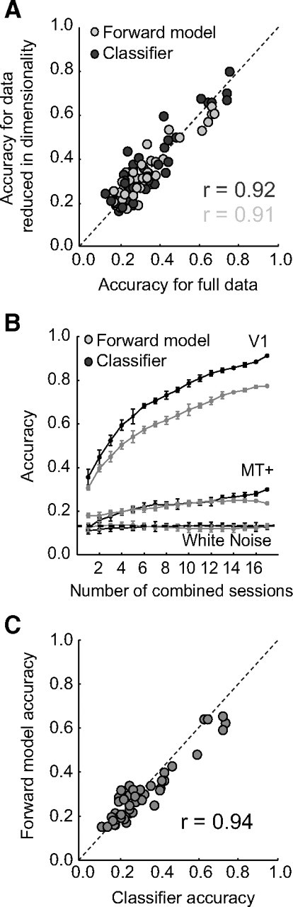
Comparison of methods. A, Comparison between decoding accuracies obtained with the full data (dimensionality = number of voxels) and accuracies obtained with the data after reducing it by means of PCA (dimensionality = number of components needed to explain 68% of the variance). Each point represents average decoding accuracy for one observer and ROI. Dark symbols, Maximum likelihood classifier. Light symbols, Forward model. Correlation coefficients (r values), Correlation in decoding accuracy between the full data and the reduced data for each decoder. B, Decoding accuracies obtained by combining data across sessions. Increasing the number of sessions dramatically increased V1 accuracies but only slightly increased MT+ accuracies. Replacing the data with white noise yielded chance performance. Error bars indicate SDs across runs (with 1 run at a time left out of training and used for testing accuracy). Dark curves and symbols, Maximum likelihood classifier. Light curves and symbols, Forward model classifier. C, Correlation between maximum likelihood classification and forward modeling classification accuracies. Each point corresponds to the mean decoding accuracy for one observer and ROI. Correlation coefficient (r value), Correlation in decoding accuracy between maximum likelihood classifier and forward model.

In a separate analysis, we determined the effect of combining different numbers of sessions on decoding accuracy. We determined the decoding accuracy (for details, see below) for V1 and MT+ to random subsets of all available sessions, which totaled 18 across observers. As an additional control, we replaced the estimated response amplitudes by white noise. Decoding accuracy for V1 increased dramatically by combining more sessions, resulting in near-perfect classification (Fig. 2B). In contrast, noise remained unclassifiable, no matter how many sessions were added. Decoding accuracy for MT+ increased only slightly as more sessions were combined; even with 18 combined sessions, MT+ decoding accuracy was only ∼25% compared with >80% for V1.

Classification.

Classification was performed with a eight-way maximum likelihood classifier, implemented by the Matlab (MathWorks) function “classify” with the option “diaglinear.” The distributed spatial pattern of response amplitudes to a single color can be described as a point in a multidimensional space, in which each dimension represents responses from a voxel (or a PCA component score, corresponding to a linear combination of voxel responses). Accurate decoding is possible when the responses to each color form distinct clusters within the space. The maximum likelihood classifier optimally separates trials belonging to each of the eight different colors, if the response variability in each voxel is normally distributed, and statistically independent across voxels (noting that PCA is an orthonormal transform so that, if the noise is normally distributed and statistically independent across voxels, then it is also normally distributed and statistically independent across PCA scores). Because the number of voxels (or PCA components), m, was large relative to the number of repeated measurements, n, the computed covariance matrix would have been a poor estimate of the real covariance. This would have made the performance of the classifier unstable, because it relied on inversion of this covariation matrix. We, therefore, ignored covariances between voxels and modeled the responses as being statistically independent across voxels. Although noise in nearby voxels was likely correlated, the independence assumption, if anything, was conservative; including accurate estimates of the covariances (if available) would have improved the decoding accuracies.

Using a leave-one-out validation, we excluded the responses from one run and trained the classifier on the estimated response amplitudes from the remaining runs. The number of runs differed between observers, creating train/test ratios between 0.875 (7 of 8 runs) and 0.90 (9 of 10 runs). Because every run yielded one estimate for each color, we obtained a prediction for each of the eight colors per run. The number of correct predictions for each run determined the accuracy for that run. Combining accuracies across runs allowed us to determine the statistical significance of the prediction accuracy. Because accuracies are not normally distributed, because they are restricted between 0 and 1, we performed a nonparametric permutation test. For each ROI and observer, we assigned random labels to the training data and obtained an accuracy from the test data. Repeating this 1000 times yielded a distribution of accuracies, according to the null hypothesis that stimulus color could not be classified. Accuracies computed with the correctly labeled training data were then considered statistically significant if they were higher than the 97.5 percentile of the null distribution (i.e., two-tailed permutation test). Similar results were obtained with a standard Student's t test, and both supported the same conclusions.

Forward model and reconstruction.

In addition to classification, we defined a forward model to decode and reconstruct color from the spatially distributed patterns of voxel responses. The forward model assumed that each voxel contained a large number of color-selective neurons, each tuned to a different hue. We characterized the color selectivity of each neuron as a weighted sum of six hypothetical channels, each with an idealized color tuning curve (or basis function) such that the transformation from stimulus color to channel outputs was one-to-one and invertible. The shape of the tuning curves was selected (as described below) so that the response tuning of any one neuron could be expressed as a weighted sum of the six basis functions. We further assumed that the response of a voxel was proportional to the summed responses of all the neurons in that voxel and hence that the response tuning of each voxel was a weighted sum of the six basis function. Each basis function was a half-wave rectified (all negative values were set to 0) and squared sinusoid, as a function of hue, in CIE L*a*b* space (Fig. 3A,B). The rectification approximated the effect of spike threshold for cortical neurons with low spontaneous firing rates, and the squaring made the tuning curves narrower. For our stimulus set (individual colors of fixed color contrast, presented one at time), this model of color selectivity is a close approximation to more elaborate models of cortical color tuning (Solomon and Lennie, 2007). A rectified and squared sinusoidal tuning curve with any possible hue preference (i.e., intermediate to the six basis functions) can be expressed exactly as a weighted sum of the six basis functions (Freeman and Adelson, 1992). The hue preferences of the six channels need not have been evenly spaced, as long as they were linearly independent (Freeman and Adelson, 1992). Although a circular space can be represented by two channels with sinusoidal tuning curves, the rectification and squaring operations led to the requirement of six channels. The half-wave rectified and squared basis functions were more selective (narrower) than sinusoidal tuning curves and strictly positive. If the basis functions were broader, then fewer channels would have been needed. If narrower, then more channels would have been needed. Saturation and luminance were not modeled, because our stimuli did not vary along those dimensions. The channel outputs for any stimulus color were readily computed from the basis functions (the tunings curves of the hypothetical channels).

Figure 3.

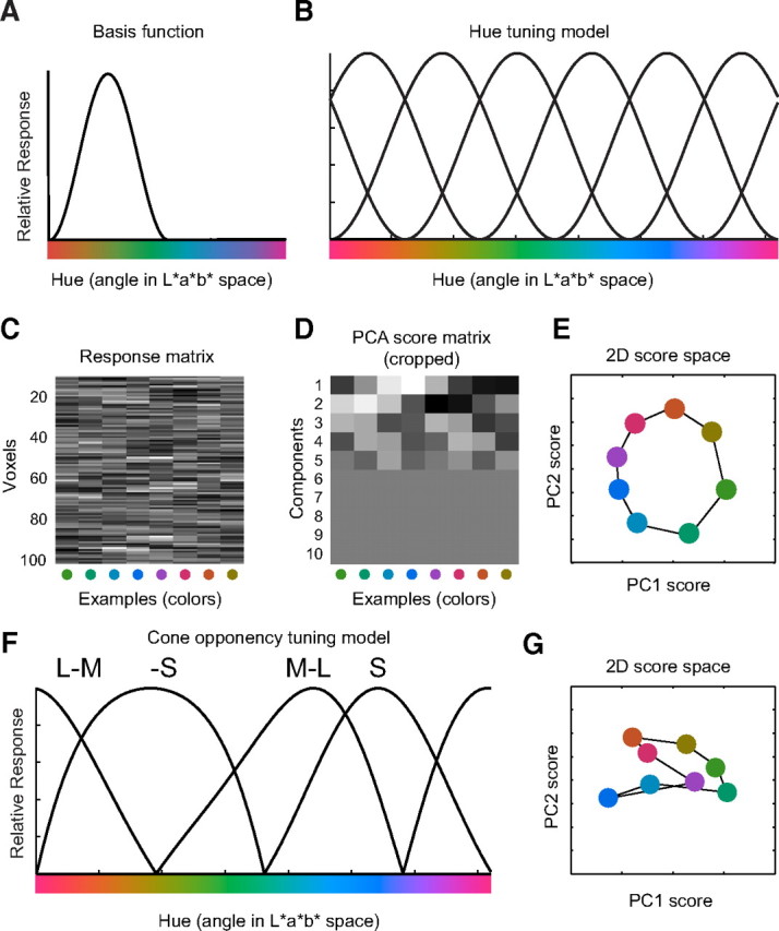
Forward model. A, Idealized color tuning curve, modeled as a half-wave rectified and squared sinusoid. B, The response of a voxel was fitted with a weighted sum of six idealized color tuning curves, evenly spaced around the color circle, in CIE L*a*b* space. C, Simulated response amplitude matrix, for each voxel and each color. D, Matrix of principal component scores, computed by projecting the vector of response amplitudes (across voxels) onto each of the principal component vectors, ordered by the amount of variance they explain in the original response amplitudes. E, Plotting the first two principal component scores as coordinate pairs reconstructs the original color space. F, Cone-opponency model. LMS cone responses were calculated for the stimulus colors. Four cone-opponency channels (M–L, L–M, −S, and +S) were computed from the cone responses, half-wave rectified. G, The first two principal components of the simulated cone-opponency responses revealed results similar to those observed in V1.

The data (the estimated voxel response amplitudes) were partitioned in train (B₁) and test sets (B₂), as for the classification analysis, and the analysis proceeded in two stages (train and test). In the first stage of the analysis, the training data were used to estimate the weights on the six hypothetical channels, separately for each voxel. With these weights in hand, the second stage of analysis computed the channel outputs associated with the spatially distributed pattern of activity across voxels evoked by each test color, and the resulting channel outputs were associated with a stimulus color. Let k be the number of channels, m be the number of voxels, and n be the number of repeated measurements (i.e., eight colors times the number of runs). The matrix of estimated response amplitudes in the training set (B₁, m × n) was related to the matrix of hypothetical channel outputs (C₁, k × n) by a weight matrix (W, m × k):

The least-squares estimate of the weights was computed using linear regression:

The channel responses (C₂) for the test data (B₂) were then estimated using the weights (Ŵ):

Finally, color was decoded by comparing the estimated channel outputs Ĉ₂ to the known channel outputs for each color. The decoded color was that which produced channel outputs with the highest correlation to those estimated from the spatially distributed pattern of voxel response amplitudes, taking into account the different weightings of the channels in each voxel. This procedure effectively reduced the dimensionality of the data from the number of voxels to six (the number of hypothetical channels). Statistical significance of the decoding accuracies was determined using the same two-tailed permutation test as used to compute statistical significance of the classification accuracies. Despite the additional data reduction, the decoding accuracies obtained using the forward model were comparable with those from the conventional classifier (Fig. 2C). The decoded colors were highly correlated (r = 0.94) between the two approaches.

The forward model enabled not only decoding (selecting one of the eight stimulus colors) but also reconstruction of stimulus colors from the test data, as the transformation from stimulus color to channel outputs was one-to-one and invertible. Instead of matching the estimated channel outputs to those of the eight stimulus colors, we created a lookup table of channel outputs for a total of 360 different hues. The reconstructed color was that with channel outputs that mostly closely matched (highest correlation) the channel outputs that were estimated (Eq. 3) from the spatially distributed pattern of voxel response amplitudes.

A more important test of the reconstruction was to remove test colors from the training data, so that these stimuli were novel during testing. We again separated the data into test (one run) and training data (the remaining runs). All measured responses evoked by one of the eight colors were removed from the training data. We then trained the forward model (i.e., estimated the weights) on the training data and performed the decoding and reconstruction of the left-out color in the test data. This process was repeated by cycling through all eight colors, leaving one out at a time. Because there was one response amplitude per color for each run and we left one color out at a time, we computed the accuracy of predicting a single novel color as the fraction of runs in which it was predicted correctly. A mean accuracy and the statistical significance of that accuracy being above chance were computed by combining the accuracies of all eight colors.

Deriving neural color spaces with PCA.

In addition to dimensionality reduction, PCA provided a means for inferring a color space from the spatially distributed patterns of activity in each visual area. Assuming that the fMRI voxels exhibited some degree of color tuning, we hypothesized that the ensemble of responses should have been reducible to two principal component scores that jointly described a neural color space. The intuition was that the covariation in the color selectivity of the voxels led to covariation in their responses. PCA characterized this covariation. Figure 3B–D illustrates the approach with simulated data, synthesized according to the forward model described above. Specifically, we started with the eight colors used in our experiments. These colors originated from a two-dimensional circular color space, because our stimuli were varied only in terms of hue, not in terms of saturation or luminance (Fig. 1A). As discussed above, this space could be encoded completely and unambiguously by six idealized channels (rectified and squared sinusoids) (Fig. 3B). Random weights on each channel were assigned to each individual voxel. The response amplitude of each voxel to each color was simulated as the weighted sum of the activity of each channel to the color (Fig. 3C). We then computed the principal components of the resulting m × n matrix of response amplitudes (where m was the number of simulated voxels and n = 8 was the number of colors). Projecting the original response amplitudes onto these principal components created a new m × n matrix of principal component scores, sorted by the amount of variance they explained within the original response amplitude matrix (Fig. 3D). By considering the values of the first two principal component scores for each color as a coordinate pair, we reconstructed the original circular color space (Fig. 3E). Response amplitudes from a single session in our real data formed m × n matrices, where m was the number of voxels in the ROI and n = 64 was the number of examples (8 stimulus colors × 8 runs). These matrices were stacked across observers and sessions as described above, yielding a matrix of size M × n where M was the total number of voxels in the ROI summed across sessions. Thus, in the real data, we had eight PCA score coordinate pairs corresponding of the same color, equal to the total number of runs. A centroid of the PCA scores was computed for each set of same-color examples.

The resulting color spaces were quantified in terms of clustering and progression. The clustering measure quantified the amount of within-color clustering by computing the distances from each PCA score coordinate pair to each of the eight (number of stimulus colors) centroids. Sorting these distances, we determined the nearest eight (number of runs and hence number of examples per color) to each centroid. For high clustering, we expected that all eight would correspond to the same color as the centroid. The clustering measure equaled the proportion of these same-color coordinates (of eight) closest to each centroid, averaged over all eight centroids. The progression measure determined the two closest neighboring centroids to each of the eight color centroids. If either one of the neighbors represented the neighboring color in perceptual color space, we added 1 to the progression measure. If both of the neighbors represented the neighboring color in perceptual color space, we added 2. The maximum possible value, when the space was indeed circular, was 16 (number of colors × 2). By the dividing the measure by 16, we bounded the progression measure between 0 and 1. Although ad hoc, these measures were one means of capturing the intuition for the clustering and progression that was expected for cortical representations that reflected perceptual color space. The chance level of progression and clustering of any dataset was computed by a permutation test; we computed the distribution of progression and clustering measures for 1000 randomly relabeled datasets and determined the 97.5 percentile (two-tailed permutation test) of that distribution. Clustering and progression measures in the real data were considered significant when they exceeded this value.

This color space analysis went well beyond the PCA data reduction mentioned above by reducing to two dimensions. High clustering and progression scores were expected only if the signal-to-noise ratio (SNR) of the measurements was sufficiently high, such that the variability (and covariation) in the fMRI responses reflected primarily the underlying neural responses to the different stimulus colors. In contrast, if the fMRI measurements were dominated by noise, then this analysis would have yielded a random color space, with low clustering and progression values.

Visual stimulus presentation.

Visual stimuli were presented with an electromagnetically shielded analog liquid crystal diode (LCD) flat-panel display (NEC 2110; NEC) with a resolution of 800 × 600 pixels and a 60 Hz refresh rate. The LCD monitor was located behind the scanner bore and was viewed by observers through a small mirror, at a distance of 150 cm creating a field of view of 16° × 12° visual angle. The monitor was calibrated using a Photo Research PR650 SpectraColorimeter. By measuring the red, green, and blue spectral density functions at different luminances, we derived the necessary conversion matrices (Brainard, 1996) to linearlize the gamma function of the monitor as well as to be able to convert any desired color space coordinate to the appropriate setting of the red, green, and blue guns of the monitor.

MRI acquisition.

MRI data were acquired on a Siemens 3 T Allegra head-only scanner using a head coil (NM-011; NOVA Medical) for transmitting and a four-channel phased array surface coil (NMSC-021; NOVA Medical) for receiving. Functional scans were acquired with gradient recalled echo-planar imaging to measure blood oxygen level-dependent changes in image intensity (Ogawa et al., 1990). Functional imaging was conducted with 27 slices oriented perpendicular to the calcarine sulcus and positioned with the most posterior slice at the occipital pole (repetition time, 1.5 s; echo time, 30 ms; flip angle, 75°; 3 × 3 × 3 mm; 64 × 64 grid size). A T1-weighted magnetization-prepared rapid gradient echo (MPRAGE) (1.5 × 1.5 × 3 mm) anatomical volume was acquired in each scanning session with the same slice prescriptions as the functional images. This anatomical volume was aligned using a robust image registration algorithm (Nestares and Heeger, 2000) to a high-resolution anatomical volume. The high-resolution anatomical volume, acquired in a separate session, was the average of several MPRAGE scans (1 × 1 × 1 mm) that were aligned and averaged and used not only for registration across scanning sessions but also for gray matter segmentation and cortical flattening (see below).

Defining visual cortical areas.

Visual cortical areas were defined using standard retinotopic mapping methods (Engel et al., 1994, 1997; Sereno et al., 1995; Larsson and Heeger, 2006). High-contrast radial checkerboard patterns were presented either as 90° rotating wedges or as expanding and contracting rings. A scanning session consisted of six to eight runs of clockwise (CW) or counterclockwise (CCW) (three or four of each) rotating wedge stimuli and four runs of expanding or contracting (two of each) ring stimuli. Each run consisted of 10.5 cycles (24 s per cycle, total of 168 time points) of stimulus rotation (CW/CCW) or expansion/contraction. Preprocessing consisted of motion compensation, linear detrending, and high-pass filtering (cutoff of 0.01 Hz). The first half-cycle of response was discarded. Time series from all runs were advanced by two frames, and the response time series for counterclockwise wedges and contracting rings were time reversed and averaged with responses to clockwise wedges and expanding rings, respectively. The Fourier transforms of the resulting time series were obtained, and the amplitude and phase at the stimulus frequency were examined. Coherence was computed as the ratio between the amplitude at the stimulus frequency and the square root of the sum of squares of the amplitudes at all frequencies. Maps of coherence and phase were displayed on flattened representations of the cortical surface. For each observer, the high-resolution anatomical volume was segmented and computationally flattened using the public domain software SurfRelax (Larsson, 2001). Visual area boundaries were drawn by hand on the flat maps, following published conventions (Larsson and Heeger, 2006), and the corresponding gray matter coordinates were recorded. There is some controversy over the exact definition of human V4 and the area just anterior to it (Tootell and Hadjikhani, 2001; Brewer et al., 2005; Hansen et al., 2007). We adopted the conventions proposed by Wandell et al. (2007). Visual areas V3A and V3B were combined for the purpose of this study into a single V3AB ROI because the boundary between V3A and V3B was not clearly evident in every observer. Area MT+ (the human MT complex) was defined, using data acquired in a separate scanning session, as an area in or near the dorsal/posterior limb of the inferior temporal sulcus that responded more strongly to coherently moving dots relative to static dots (Tootell et al., 1995), setting it apart from neighboring areas LO1 and LO2 (Larsson and Heeger, 2006).

Results

Classification

Stimulus colors were decoded from the spatially distributed patterns of activity in each of several visual cortical areas, using an eight-way maximum likelihood classifier (see Materials and Methods). We trained the classifier on data from all but one run and tested the classifier on the remaining run, leaving each run out in turn. Decoding performance was high and significantly above chance in all observers for visual areas V1, V2, and V3 and in the majority of observers for V4 and VO1 (Fig. 4A, Table 1). Decoding colors on the basis of LO1, LO2, V3AB, and MT+ responses proved to be inaccurate, reaching accuracies significantly higher than chance in only one or two observers. Averaging across observers revealed a similar pattern (Fig. 4A, Table 1). Combining data across observers before classification yielded decoding accuracies above those obtained from any one observer alone. Decoding on the basis of V1 activity was nearly perfect (93% relative to 12.5% chance performance), whereas decoding on the basis of MT+ activity was only 32% accurate. Higher decoding accuracies obtained from combining data across observers might have been driven by differences between these observers. If every observer's data allowed for the correct classification of only a limited set of colors and if these correctly classified colors differed between observers, combining data would have improved classification accuracy across all colors. Inspection of the individual classification results (data not shown) revealed that this was not the case; each observer showed comparable classification accuracies across all colors.

Figure 4.

Color decoding. A, Decoding accuracies obtained with the maximum likelihood classifier, for each visual area. Gray bars, Decoding accuracies for individual observers. Light bars, Mean across observers. Dark bars, Accuracies obtained by combining the data across observers before classification. *p < 0.05, visual areas for which accuracies were significantly above chance in all observers (2-tailed permutation test); ^†p < 0.05, areas for which accuracies were significantly above chance in at least three of five observers. Error bars indicate SDs across runs (with 1 run at a time left out of training and used for testing accuracy). Solid line, Chance accuracy (0.125%). Dashed line, 97.5 percentile for chance accuracy, obtained by permutation tests (see Materials and Methods). The 97.5 percentiles were computed separately for each observer and visual area, but the average across observers/ROIs is shown here for simplicity. B, Decoding accuracies obtained using the forward model. Same format as in A.

Table 1.

Decoding accuracies

	V1	V2	V3	V4	VO1	LO1	LO2	V3AB	MT+
A
O1	0.73	0.46	0.63	0.64	0.25	0.36	0.25	0.18	0.18
O2	0.72	0.72	0.41	0.25	0.20	0.27	0.23	0.28	0.25
O3	0.43	0.43	0.33	0.33	0.41	0.31	0.18	0.23	0.19
O4	0.59	0.30	0.38	0.25	0.27	0.16	0.25	0.20	0.19
O5	0.40	0.22	0.28	0.21	0.21	0.17	0.11	0.14	0.21
Mean	0.56	0.42	0.39	0.33	0.27	0.25	0.20	0.20	0.20
Combined	0.93	0.73	0.73	0.73	0.48	0.32	0.39	0.23	0.32
B
O1	0.63	0.42	0.64	0.64	0.34	0.34	0.21	0.22	0.16
O2	0.66	0.59	0.33	0.22	0.20	0.22	0.17	0.27	0.30
O3	0.40	0.36	0.30	0.30	0.36	0.28	0.16	0.19	0.19
O4	0.48	0.32	0.25	0.23	0.32	0.20	0.25	0.29	0.27
O5	0.32	0.28	0.29	0.19	0.32	0.18	0.15	0.15	0.21
Mean	0.49	0.39	0.35	0.31	0.31	0.24	0.19	0.22	0.22
Combined	0.80	0.64	0.71	0.64	0.51	0.41	0.43	0.34	0.36

A, Decoding accuracies obtained with the maximum likelihood classifier, for each visual cortical area. Accuracies are listed separately for each individual observer (O1–O5), averaged across observers (Mean), and when data were combined across all observers before classification (Combined). Bold font indicates decoding accuracies that were significantly higher than chance as determined by a two-tailed permutation test (p < 0.05; see Materials and Methods). Accuracies were significantly greater than chance for V1, V2, and V3 in all observers and for areas V4 and VO1 in at least three of five observers. B, Decoding accuracies obtained using the forward model, showing a very similar pattern of (statistically significant) decoding accuracies as was found for the classifier.

Forward model, decoding

Similar decoding performance was found using a simple forward model of cortical color selectivity (Fig. 4B, Table 1). Briefly, we modeled the response of each voxel as a weighted sum of the activity of six color-selective channels with idealized tuning curves. Subdividing the data into training and test sets, we used the training set to estimate the weights on the six channels, separately for each voxel. We then used the weights to estimate the channel outputs from the spatially distributed pattern of voxel responses. The channel outputs for each of the eight stimulus colors were computed from the tuning curves of the hypothetical channels and compared with the channel outputs estimated from the data (for details, see Materials and Methods). Decoding accuracies were high and statistically significant in all observers for V1, V2, and V3 and in the majority of the observers for areas V4 and VO1. Decoding accuracies for LO1, LO2, V3AB, and MT+ were higher than chance in only a minority of the observers. Averaging across observers revealed a similar pattern. As with the maximum likelihood classifier, combining across observers into a single dataset before decoding yielded higher accuracies than those obtained from any one observer alone. Even so, decoding on the basis of V3AB or MT+ activity was only ∼35% accurate.

Forward model, reconstruction

The benefit of using a forward model is that it allowed us to reconstruct stimulus color from the spatially distributed patterns of cortical activity, because the transformation from stimulus color to channel outputs was one-to-one and invertible. The reconstruction analysis began with the same steps as forward model decoding. However, instead of determining which of eight stimulus colors was best correlated with the channel outputs, we created a lookup table of channel outputs for an arbitrarily large number of different hues (see Materials and Methods). For visual areas with high decoding accuracy, colors were reconstructed accurately (Fig. 5) (supplemental Fig. 3, available at www.jneurosci.org as supplemental material). There were occasional large errors in reconstruction, but such mistakes were infrequent. In contrast, colors reconstructed using MT+ activity differed substantially from the actual stimulus colors (supplemental Fig. 3, available at www.jneurosci.org as supplemental material).

Figure 5.

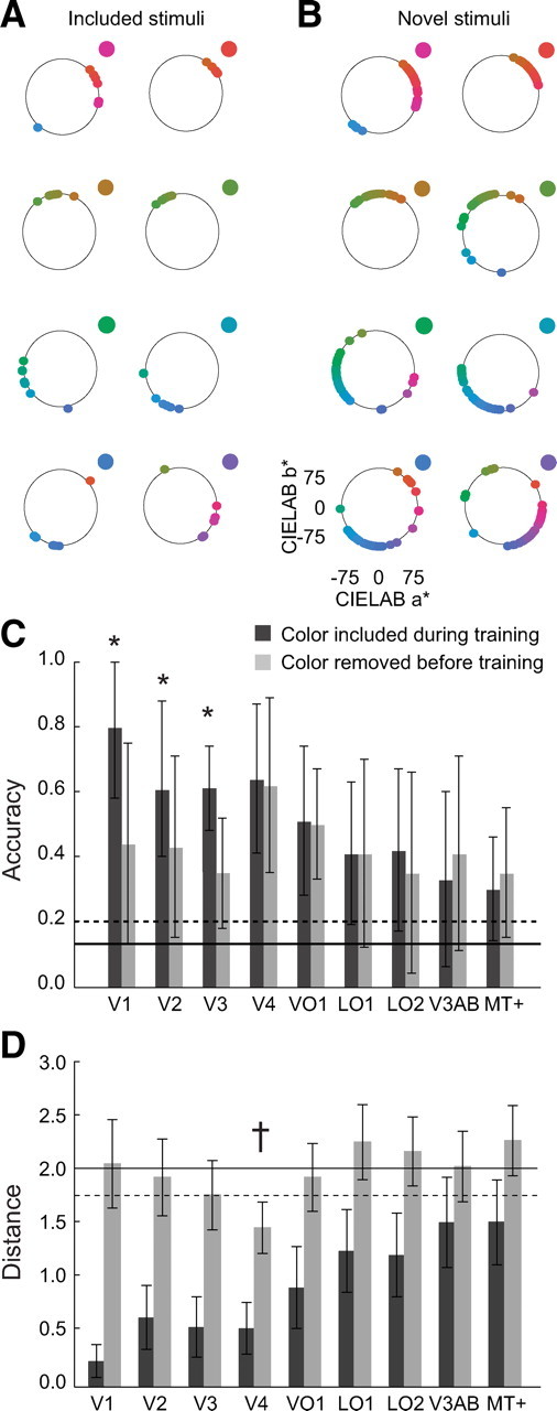
Reconstruction. A, Color reconstruction on the basis of V4 activity. Each point represents the color reconstructed for one run, using combined data from all sessions and observers, plotted in CIE L*a*b* space. The reconstructed colors from all sessions and observers cluster near the actual stimulus color, indicated in the top right of each panel. B, Reconstruction of novel colors, not included in training the forward model. Reconstructed colors again cluster near the actual stimulus color but with more spread than in A. C, Forward model decoding accuracies for included and novel colors. Error bars indicate SD of the accuracies over runs. *p < 0.05, visual areas for which there was a statistically significant difference when the test color was excluded from training (paired-sample t test). Solid line, Chance accuracy (0.125%). Dashed line, 97.5 percentile for chance accuracy, obtained by permutation tests (identical to Fig. 4). Areas V1, V2, and V3 show a significant decrease in decoding accuracy for novel colors, whereas areas V4 and VO1 show highly similar decoding accuracies for both included and novel colors. The accuracies for included colors in this figure are similar but not identical to the combined accuracies shown in Figure 4B. Each run is associated with one example per color. If we remove one color from training at a time and we leave one run out at a time, we can only predict one example per run (the example associated with the color excluded from training). The remaining colors in the run are not novel. Thus, for fair comparison, we determined the accuracy for included colors in the same way. D, Performance of the maximum likelihood classifier on included (black bars) and novel (gray bars) colors, quantified as the average distance between the color predicted by the maximum likelihood classifier and the novel color presented. Small distances indicate that the classifier predicted colors as perceptually similar, neighboring colors. The maximum distance was 4 (classifying a novel color as the opposite color on the hue circle), and the minimum distance in the case of included colors was 0 (correctly classifying a included color), or, in the case of novel colors, the minimum distance was 1 (classifying a novel color as its immediate neighbor). Error bars indicate SDs across runs (with 1 run at a time left out of training and used for testing accuracy). Solid line, Median distance as expected by chance. Dashed line, Statistical threshold (p < 0.05, two-tailed permutation test). ^†p < 0.05, visual areas for which the measured distance for novel colors was statistically smaller than expected by chance.

A more important test of the reconstruction was to remove colors from the training data, so that these stimuli were novel during testing (for details, see Materials and Methods). For V4, novel colors were reconstructed well, almost as well as when the colors were included during training, albeit with a larger spread (Fig. 5) and likewise for VO1. For V1, V2, and V3, however, reconstruction of novel colors was less accurate than that for colors that were included during training. Reconstruction for the remaining visual areas was generally poor and did not depend much on whether the colors were including during training. Decoding novel stimulus colors with the forward model as one of the eight used stimulus colors revealed a similar pattern. The highest decoding accuracies for novel colors were found for V4 and VO1 (Fig. 5C). For V1, V2, and V3, decoding accuracies were significantly lower (as determined by a paired-sample t test) for novel colors than for trained colors (V1 mean accuracy: trained colors, 0.81; novel colors, 0.45; p = 0.01; V2 mean accuracy: trained colors, 0.64; novel colors, 0.43; p = 0.03; V3 mean accuracy: trained colors, 0.61; novel colors, 0.34; p = 0.01). For the remaining visual areas, decoding accuracies were not significantly different (p > 0.05) between included and novel stimulus colors (Fig. 5C). In addition, we determined the output of the classifier to novel stimuli. Although the classifier cannot correctly classify a novel stimulus, we nevertheless assessed whether it classified a novel color as a neighboring color. To quantify this, we computed the distance between the novel color presented and the color predicted by the classifier and compared this with the distances obtained when colors were included during training. Figure 5D mimicked the results shown in Figure 5C: for V1, V2, and V3, included colors were decoded accurately, as indicated by the small distance between the color presented and the color predicted by the classifier. However, when the same color was novel, the distance increased substantially (associated with lower decoding accuracies), even becoming statistically insignificant. The measured distance for novel colors was statistically significant (smaller than chance) only for V4 (Fig. 5D), again in line with the results obtained with the forward model, for which V4 showed the highest accuracy in decoding novel colors.

Neural color space revealed by principal component analysis

In V4 and VO1, the first two principal components (main source of variation) of the responses revealed a progression through perceptual color space, with perceptually similar colors evoking the most similar responses (Fig. 6A) (supplemental Fig. 4A, available at www.jneurosci.org as supplemental material). The spatially distributed patterns of fMRI responses, combined over all sessions and observers, corresponding to each stimulus color in each run, were projected onto the two-dimensional vector space spanned by the first two principal components. There are two important observations about these projected responses (which we refer to as the PCA scores). First, the scores from different runs, but corresponding to the same stimulus color, clustered together. The high clustering of the scores from different runs found in V1, relative to other visual areas, indicated more reliable and consistent responses to the different colors over runs in this area. In turn, these reliable responses enabled accurate classification. Second, and more importantly, there was a progression through color space. In V4, this progression was nearly circular and was not self-intersecting. VO1 showed a similar circular space, with only a single outlier. This was not the case for any of the other visual cortical areas (Fig. 6A) (supplemental Fig. 4A, available at www.jneurosci.org as supplemental material), including V1. Although V1 exhibited a tighter clustering then V4 (and VO1) and V1 decoding accuracy was correspondingly higher than that in V4 (and VO1), neighboring clusters from V1 did not always correspond to perceptually similar colors. The color space derived from MT+ responses resembled results obtained using white noise for the responses, with relatively little clustering and with the cluster centroids near the origin of the space.

Figure 6.

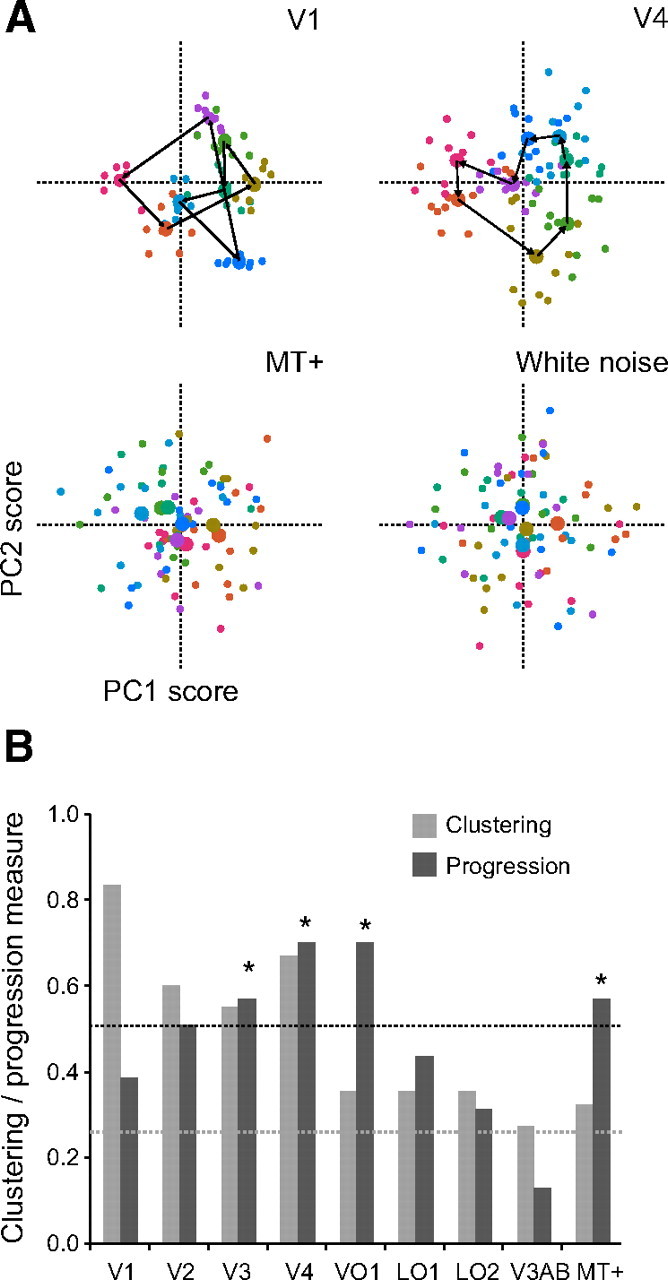
Neural color spaces. A, Color spaces derived from the covariation, across voxels, in the responses to different stimulus colors, using data combined over all sessions and observers. In V4, the first two principal components (main source of variation) reveal a nearly circular progression (not self-intersecting) through color space, with similar colors evoking the most similar responses. This is not the case for V1 or MT+ activity, nor for white noise. Note, however, that V1 shows a more robust clustering of PCA scores, relative to the other areas. B, Clustering and progression of the color spaces derived from activity in each visual cortical area. Dashed lines, Chance levels for the progression (black) and clustering (gray) measures, computed by a permutation test (see Materials and Methods). All areas show clustering significantly higher than chance (p < 0.05, two-tailed permutation test). *p < 0.05, visual areas with a progression measure higher than chance (two-tailed permutation test). The relatively high progression score in MT+ is artifactual because the cluster centers were all near the origin of the space.

These observations were quantified, separately for each visual area, by computing a measure of within-color clustering and a measure of progression through color space (see Materials and Methods). V1 exhibited the highest clustering but only modest progression (Fig. 6B). In contrast, areas V4 and VO1 showed the highest progression (significantly higher than would have been expected by chance, as determined by a permutation test; see Materials and Methods) but weaker clustering. Progression and clustering in V2 and V3 were intermediate between those for V1 and V4, but the progression and clustering were relatively low in the remaining visual areas (noting that the relatively high progression score in MT+ was artifactual because the cluster centers were all near the origin of the space).

The dissociation between the color spaces in V1 and V4 was also present for the individual observers, although not as pronounced as in the combined data (supplemental Fig. 4B, available at www.jneurosci.org as supplemental material). Across observers, treating individual differences as a random factor, we found significantly higher clustering in V1 relative to V4 (p = 0.02, paired-sample t test) and significantly higher progression in V4 relative to V1 (p = 0.04, paired-sample t test) (supplemental Fig. 4C, available at www.jneurosci.org as supplemental material).

Although the first two PCA components from V1 did not reveal a color space akin to the one found in V4, it nevertheless might have shown such a progression in combinations of later component scores, responsible for explaining a lesser amount of variance in the V1 responses. This would be expected if the main source of variation in V1 resulted from changes in, for example, subtle differences in contrast, luminance, or saturation between our colored stimuli, although our stimuli were calibrated to have equal luminance and contrast and were chosen from a perceptually homogenous color space. In an additional analysis, we computed the progression for all combinations of components. Some combinations of V1 components showed a high progression measure, but these components explained only small amounts of variance (the highest progression measure was obtained using a pair of V1 components explaining <2% of the variance of the data, whereas the first pair of V1 components explained ∼11% of variance). This indicates that the response variation attributable to variations in color were not hidden just below a signal of non-color-specific origin. Moreover, clustering was low (and consequently decoding accuracy was poor) for the pairs of V1 components that yielded high progression. Similar results were also observed for the other visual areas, excluding V4 and VO1. For V4 and VO1, the highest progression measures were found with the first two components.

The presence of high clustering but lack of progression in the PCA scores from V1 suggested that the activity was not characterized by the proposed forward model, tuned to perceptual hues. Such a model predicted a circular, progressing color space in the principal component scores. We therefore considered an alternative underlying model of tuning: cone opponency (Fig. 3F). Specifically, we calculated LMS cone responses to our stimulus colors. By subtracting L from M cone responses, we created an M–L channel. The channel was rectified (all negative values set to 0). By subtracting M from L cone responses, we created an L–M channel, also rectified. Note that these two channels would have been perfectly negatively correlated, before rectification. Finally, we created two S cone channels, modeling positive and negative S cone responses to our stimuli, relative to the activity of the L and M cones. The S cone channels (LM−S, LM+S) were also rectified. All channels were normalized to yield an identical maximum response of 1 (Fig. 3F).

Simulating our experiment using these cone-opponency channels, instead of the hue-tuned channels, reproduced some but not all of the features of the V1 responses. (1) The resulting color space showed no progression between clusters of similar colors (Fig. 3G). (2) Decoding accuracy was high for colors included in the training set but much lower for novel colors (simulation results not shown). (3) In both model and V1 responses, the green, yellow, and purple hues clustered together on one side, whereas the blue and red/orange hues were found on the other side (compare Figs. 3G, 6A). Why did the cone-opponency model exhibit this behavior, unlike the forward model with hue-tuned channels? It is not the result of the lower number of channels in the cone-opponency model (four channels) compared with the hue tuning model (six channels): a circular color space can be encoded unambigiously by four channels, provided that they have the correct shape (rectified but not squared sinusoids). Rather, the hue-tuned channels are “shiftable” (Freeman and Adelson, 1992), by which we mean that a tuning curve of the same shape but shifted to any possible preferred hue can be expressed exactly as a weighted sum of the basis functions (a subtlety here is that the basis functions need not have been evenly spaced as long as they were linearly independent). However, this is not true for the cone-opponency channels; the cone-opponent tuning curves do not cover the perceptual hue circle evenly and they are not shiftable. Our colors were defined in a space designed to be perceptually homogeneous (CIE L*a*b*). To achieve perceptual homogeneity, the space is a nonlinear transform of the underlying cone-opponency space. For example, the two greenish hues are relatively close together in CIE L*a*b* space, whereas in cone-opponency space, the response they produce is quite different (activating either mostly the L–M axis in the case of turquoise green, or mostly the LM–S axis in the case of lime green). The opposite is true as well; there is quick transition from yellow to orange and reddish hues in cone-opponency space, whereas the same transition covers a much larger portion of CIE L*a*b* space. As a result of this nonlinear transformation, if neural responses to colors chosen from a perceptual color space, such as CIE L*a*b*, are driven by a cone-opponency model, those neural responses cannot be used to reconstruct the perceptual color space, attributable to the nonlinear warping between the two spaces. The similarity between the color space reconstructed from the cone-opponency model simulation and the measured V1 responses, although tentative, suggests that, indeed, the representation of hue in V1 is incomplete. Supporting evidence for this comes from the fact V1 performs poorly in classifying novel colors compared with V4 and VO1 (Fig. 5A,B). The spatially distributed pattern of activity in V1, unlike V4 and VO1, does not allow for interpolation between colors (e.g., the pattern of responses evoked by orange is not halfway in between the patterns evoked by red and yellow).

An alternative model, based on physiological data recorded from V1 neurons (Conway, 2001), modeling responses as S–LM and L–SM channels, similarly reproduced some but not all of the observed V1 PCA scores.

In summary, the dissociation between clustering (highest in V1 and supporting the best decoding performance) and progression (highest in V4) implies a transformation from the color representation in V1 to a representation in V4 (and to a lesser extent VO1) that was closer to a perceptual color space.

Mean response amplitudes

Accurate decoding was attributable to information available in the spatially distributed pattern of responses. A priori, decoding could have relied on differences in the mean response amplitudes averaged throughout each visual area ROI. Although the stimuli were matched in terms of luminance and distance within a color space designed to be perceptually uniform, there was no guarantee that these colors would have evoked the same mean response amplitude in each of the visual areas. However, there was no evidence for any differences in the mean responses amplitudes (Fig. 7). We computed the mean response amplitudes, averaged across voxels in each ROI and each observer, and found only two instances of significant differences between the mean amplitudes evoked by different colors (Table 2A). Note that these two significant differences occurred for the same observer but that this observer showed only intermediate decoding accuracies (Fig. 4). Averaging across observers revealed no significant differences between the mean response amplitudes to different stimulus colors. Furthermore, attempting to decode colors based on the mean responses in each ROI yielded chance performance (Table 2B). Identical to the multivariate classification approach, we trained a classifier on the mean ROI responses from all but one run and tested the performance of the classifier on the remaining run. Decoding accuracies based on these mean responses were significantly higher than chance for only 5 of 45 ROIs/observers, and there was no consistency across observers. Even for those that were statistically above chance, the accuracies were still low.

Figure 7.

Mean response amplitudes. Mean response amplitudes for each of the eight colors, averaged throughout each of three representative visual area ROIs, from a representative observer. In this observer, it is clear that the mean responses were not statistically different between colors. Similar results were found for other observers/ROIs. Error bars indicate SD of mean responses, averaged across voxels, over runs. See also Table 2.

Table 2.

Mean response amplitudes

	df	V1	V2	V3	V4	VO1	LO1	LO2	V3AB	MT+
A
O1	7, 183	(0.59)	(0.32)	(0.28)	(0.66)	(0.44)	(0.52)	(0.71)	(0.68)	(0.57)
		p = 0.76	p = 0.95	p = 0.96	p = 0.70	p = 0.88	p = 0.82	p = 0.66	p = 0.69	p = 0.78
O2	7, 431	(1.38)	(0.42)	(0.18)	(0.05)	(0.44)	(0.06)	(0.33)	(0.23)	(0.26)
		p = 0.21	p = 0.89	p = 0.99	p = 0.99	p = 0.88	p = 0.99	p = 0.94	p = 0.98	p = 0.97
O3	7, 215	(1.77)	(0.81)	(0.90)	(0.67)	(0.93)	(0.34)	(0.20)	(0.84)	(1.39)
		p = 0.10	p = 0.58	p = 0.51	p = 0.70	p = 0.48	p = 0.94	p = 0.98	p = 0.56	p = 0.21
O4	7, 239	(1.93)	(1.68)	(1.37)	(2.25)	(1.31)	(1.10)	(0.98)	(0.82)	(3.38)
		p = 0.07	p = 0.11	p = 0.22	p = 0.03	p = 0.25	p = 0.37	p = 0.45	p = 0.57	p = 0.00
O5	7, 191	(0.53)	(0.17)	(0.21)	(0.25)	(0.67)	(0.31)	(1.85)	(0.30)	(0.64)
		p = 0.81	p = 0.99	p = 0.98	p = 0.97	p = 0.70	p = 0.95	p = 0.08	p = 0.95	p = 0.72
Combined	7, 143	(1.45)	(0.66)	(0.27)	(0.12)	(0.18)	(0.89)	(0.68)	(1.13)	(0.25)
		p = 0.19	p = 0.70	p = 0.96	p = 0.99	p = 0.99	p = 0.52	p = 0.68	p = 0.06	p = 0.97
B
O1		0.21	0.11	0.18	0.13	0.11	0.11	0.14	0.14	0.04
O2		0.22	0.11	0.20	0.20	0.17	0.14	0.19	0.11	0.14
O3		0.16	0.18	0.10	0.15	0.15	0.14	0.15	0.10	0.18
O4		0.11	0.09	0.16	0.20	0.14	0.11	0.07	0.13	0.13
O5		0.15	0.14	0.13	0.10	0.08	0.07	0.08	0.08	0.18
Combined		0.16	0.16	0.14	0.18	0.07	0.11	0.07	0.11	0.13

A, F statistics (parentheses) and p values for a one-way ANOVA analysis between the mean response amplitudes evoked by the different colors, across ROIs and observers. Significant results (p < 0.05) are shown in bold. First column represents the degrees of freedom per observer and the degrees of freedom for the combined analysis. Only in two cases (observer O4, V4, and MT+) were there significant differences between the mean response amplitudes evoked by the different colors. No significant differences were found when the data were combined across observers (bottom row). B, Decoding accuracies when attempting to classify colors on the basis of mean response amplitudes. For all areas, decoding accuracies are at or near chance, with accuracies significantly higher than chance only in a handful of observers/ROIs (two-tailed permutation test, p < 0.05, shown in bold).

Effect of eccentricity

Color sensitivity in the retina varies as a function of location, most notably the increase in S cones as a function of eccentricity and the complete absence of S cones in central fovea. These observations have led some to speculate that color processing is different in the fovea and periphery. To determine whether our classification results were driven by inhomogeneity in color encoding across the visual field, we isolated voxels responsive to seven different eccentricities (based on retinotopic mapping) and computed the decoding accuracy from each visual area ROI, separately for each eccentricity (supplemental Fig. 5, available at www.jneurosci.org as supplemental material). Three of the visual cortical areas exhibited significantly higher decoding accuracy at one eccentricity relative to others (V2: F_(7,55) = 3.28, p = 0.04; V4: F_(7,55) = 2.62, p = 0.02; LO2, F_(7,55) = 3.28, p = 0.04; ANOVA). However, the eccentricities at which decoding accuracies were higher differed between these three visual areas. The same analysis revealed that V3 showed a small but significant increase in decoding accuracies for larger eccentricities (F_(7,55) = 3.28, p = 0.01). Although mean decoding accuracies did not differ reliably as a function of eccentricity, there might have been a difference in accuracies between colors at different eccentricities. However, we observed no systematic shift in the classifier's ability to distinguish between different colors as a function of eccentricity (supplemental Fig. 6, available at www.jneurosci.org as supplemental material), over the range of eccentricities that we examined (between ∼0.5 and 10° of visual angle).

Discussion

We investigated how color is represented in the spatially distributed pattern of activity in visual cortex. Our results can be summarized as follows. (1) The mean responses, averaged across voxels in each visual area, were not reliably distinguishable for different stimulus colors. (2) Stimulus colors were accurately decoded from activity in V1, V2, V3, V4, and VO1, using either the conventional pattern classifier or the forward model, but decoding accuracies from LO1, LO2, V3A/B, and MT+ were not consistently above chance. (3) The forward model also reliably reconstructed novel stimulus colors not used to train the model, particularly in V4 and VO1. (4) The first two principal components (main source of variation) of the responses in V4 and VO1 (but not in V1, although decoding was most accurate in V1) revealed a progression through perceptual color space, with perceptually similar colors evoking the most similar responses. These results imply a transformation from the color representation in V1 to reflect perceptual color space in V4 and VO1.

Using conventional pattern recognition, we found that early visual areas contain information distributed across voxels that can be reliably used to decode stimulus color. This replicates a previous report of successful color classification between four unique hues in V1 (Parkes et al., 2009), but that study did not assess any of the other visual cortical areas. We found that decoding accuracies from V1 were superior to other visual areas, which makes it tempting to conclude that V1 is highly color selective, more so than V4. The decoding results on their own, however, provide only a limited basis for drawing conclusions about the color selectivity of neural responses and about the color space(s) in which neurons represent color. A high decoding accuracy obtained from a visual area (as long as the mean responses are indistinguishable between colors) implies that it contains an inhomogeneous, spatial distribution of color selectivities. It has been suggested that reliable, spatially distributed patterns of fMRI response arise from an underlying columnar architecture, at least in the case of orientation tuning (Haynes and Rees, 2005; Kamitani and Tong, 2005). There is evidence that color tuning in V1 and V2 is also spatially organized but that, unlike orientation, this tuning is both local and sparse (Xiao et al., 2003, 2007). Accurate classification and reconstruction need not arise from an underlying classic columnar architecture, but it does indicate that there are neurons with different color selectivities that are arranged inhomogenously, leading to a bias in color preferences as measured at the resolution of the fMRI voxels. A similar conclusion was reached by Parkes et al. (2009). A visual area with a low decoding accuracy, however, might nonetheless have a large population of color-selective neurons. The accuracy might be low because the SNR of the measurements was poor or because neurons with different color selectivities are evenly distributed within each voxel, yielding no differences in the responses to the different stimulus colors. In addition, the statistics associated with the accuracies can be misleading. Decoding accuracies from VO1 and LO2 were similar, but decoding from VO1 was significantly above chance whereas decoding from LO2 was not statistically significant. It would be incorrect to conclude, because of small differences straddling a threshold for statistical significance, that VO1 represents color in its distributed pattern of responses, whereas LO2 does not. We therefore complemented the conventional classification approach with two additional analyses: forward modeling and PCA.

Decoding accuracies obtained with the forward model were comparable with conventional classification. In addition, the forward model enabled decoding and reconstructing novel stimulus colors that were excluded from training. An analogous model-based approach has been shown to be capable of classifying novel natural images from cortical activity (Kay et al., 2008). Reconstructing stimuli directly from brain activity has also been demonstrated for binary black and white patterns (Miyawaki et al., 2008). We applied a much simpler forward model, designed only to capture color tuning, allowing us to reconstruct any color from observed patterns of activity, and compare these reconstructed colors with the actual stimulus colors.

The dissociation between the decoding results and the principal components analysis provides the basis for our main conclusion that there must be a transformation from the color representation in V1 to that in V4 (and adjacent VO1). Our stimuli varied in hue, around a circle in color space. We therefore focused on the first two principal components that suffice to span a subspace containing a circle. The scores of the first two PCA components from V4 revealed a progression through perceptual color space that was not self-intersecting. This was not the case in V1, although decoding was more accurate in V1 than in V4. In fact, no combination of V1 components (nor in any visual areas other than V4 and VO1), which explained a substantial portion of variance in the response amplitudes, showed a reliable progression through color space. This dissociation could not have been attributable to higher SNR in V4 than in V1, which would have yielded higher decoding accuracy in V4 than in V1 (opposite of what was observed). Likewise, it could not have been attributable to a larger subpopulation of color-selective neurons in V4 than in V1, which would have contributed to higher SNR in V4 than in V1, again yielding higher decoding accuracy in V4 than in V1, nor could it have been attributable to greater spatial inhomogeneity of color selectivities in V4 than in V1 for the same reason. It is informative that the first two scores (the main source of variation) of V4 and VO1 activity showed this progression through color space. This would not have occurred if these areas exhibited noisy responses or weak color selectivity. The fact that the main source of response variation in V4 showed a clear progression through perceptual color space supports the hypothesis that V4 neurons are hue tuned in a manner very similar to our proposed forward model.

Obviously, the lack of progression in the early visual areas (in particular V1) should not be taken as an indication that these areas are colorblind. Numerous studies have reported the existence of chromatic signals within most visual areas, using a variety of techniques (Dow and Gouras, 1973; Gouras, 1974; Yates, 1974; Thorell et al., 1984; Kleinschmidt et al.,1996; Engel et al., 1997; Kiper et al., 1997; Johnson et al., 2001; Shipp and Zeki, 2002; Solomon and Lennie, 2007). An alternative model of color selectivity, based on cone-opponent tuning rather than hue tuning, reproduced many features of the non-circular and self-intersecting color space derived from the V1 PCA scores.

The decoding of novel colors with the forward model provided supporting evidence for a perceptual color space representation in V4 (and VO1) but not in the other visual areas (including V1). When all colors were included during training, decoding accuracies from V1, V2, and V3 were higher than V4. However, although decoding accuracies from V4 were unaffected by removing the test color during training, we found a significant drop in the decoding accuracies from V1, V2, and V3. Hence, the spatially distributed representations of color in V4 supported “interpolation” to decode a stimulus color based on the responses to perceptually similar colors. These results are predicted by the hypothesis that the spatially distributed pattern of activity evoked by a test color in V4 was approximately halfway between those evoked by the two perceptually flanking colors. This difference across visual areas cannot be attributable to a better fit of the forward model in V4 because the decoding accuracy was higher in V1 than in V4 when all colors were used during training.

The experimental colors used in the present study were chosen from an isoluminant plane within the CIE L*a*b* space, restricting the dynamic range of the colors. Therefore, the stimuli did not represent the best perceptual exemplars of the unique hues. As such, it is conceivable that our results actually underestimated the decoding (as well as clustering and progression measures) obtainable from visual areas encoding perceptual hues, because the stimuli did not maximize differences and uniqueness in perceptual color space.

Nonetheless, our results support the hypothesis that V4 and VO1 play a special role in color vision and the perception of unique hues (Stoughton and Conway, 2008). In particular, macaque physiological recordings have found color-biased spots (“globs”) in posterior inferior temporal cortex (encompassing V4) in which a large proportion of the cells exhibit luminance invariant color tuning (Conway et al., 2007) and a tendency to be tuned more frequently to unique hues (Stoughton and Conway, 2008). The spatial distribution of neural activity in these ventral stream cortical areas, at least when measured at the spatial scale of fMRI voxels, exhibits a strong and reliable dependence on variations in stimulus color that covaries with perceived color.

References

- Bartels A, Zeki S. The architecture of the colour centre in the human visual brain: new results and a review. Eur J Neurosci. 2000;12:172–193. doi: 10.1046/j.1460-9568.2000.00905.x. [DOI] [PubMed] [Google Scholar]
- Boynton GM, Engel SA, Glover GH, Heeger DJ. Linear systems analysis of functional magnetic resonance imaging in human V1. J Neurosci. 1996;16:4207–4221. doi: 10.1523/JNEUROSCI.16-13-04207.1996. [DOI] [PMC free article] [PubMed] [Google Scholar]
- Brainard DH. Cone contrast and opponent modulation color spaces. In: Kaiser P, Boynton RMB, editors. Human color vision. Washington, DC: Optical Society of America; 1996. pp. 563–579. [Google Scholar]
- Brewer AA, Liu J, Wade AR, Wandell BA. Visual field maps and stimulus selectivity in human ventral occipital cortex. Nat Neurosci. 2005;8:1102–1109. doi: 10.1038/nn1507. [DOI] [PubMed] [Google Scholar]
- Commission Internationale de l'Eclairage. Colorimetry. Ed 2. Vienna: Commission Internationale de l'Eclairage; 1986. CIE No. 152. [Google Scholar]
- Conway BR. Spatial structure of cone inputs to color cells in alert macaque primary visual cortex (V1) J Neurosci. 2001;21:2768–2783. doi: 10.1523/JNEUROSCI.21-08-02768.2001. [DOI] [PMC free article] [PubMed] [Google Scholar]
- Conway BR, Moeller S, Tsao DY. Specialized color modules in macaque extrastriate cortex. Neuron. 2007;56:560–573. doi: 10.1016/j.neuron.2007.10.008. [DOI] [PMC free article] [PubMed] [Google Scholar]
- Dale AM. Optimal experimental design for event-related fMRI. Hum Brain Mapp. 1999;8:109–114. doi: 10.1002/(SICI)1097-0193(1999)8:2/3<109::AID-HBM7>3.0.CO;2-W. [DOI] [PMC free article] [PubMed] [Google Scholar]
- Derrington AM, Krauskopf J, Lennie P. Chromatic mechanisms in lateral geniculate nucleus of macaque. J Physiol. 1984;357:241–265. doi: 10.1113/jphysiol.1984.sp015499. [DOI] [PMC free article] [PubMed] [Google Scholar]
- Dinstein I, Gardner JL, Jazayeri M, Heeger DJ. Executed and observed movements have different distributed representations in human aIPS. J Neurosci. 2008;28:11231–11239. doi: 10.1523/JNEUROSCI.3585-08.2008. [DOI] [PMC free article] [PubMed] [Google Scholar]
- Dow BM, Gouras P. Color and spatial specificity of single units in Rhesus monkey foveal striate cortex. J Neurophysiol. 1973;36:79–100. doi: 10.1152/jn.1973.36.1.79. [DOI] [PubMed] [Google Scholar]
- Engel S, Zhang X, Wandell B. Color tuning in human visual cortex measured with functional magnetic resonance imaging. Nature. 1997;388:68–71. doi: 10.1038/40398. [DOI] [PubMed] [Google Scholar]
- Engel SA, Rumelhart DE, Wandell BA, Lee AT, Glover GH, Chichilnisky EJ, Shadlen MN. fMRI of human visual cortex. Nature. 1994;369:525–527. doi: 10.1038/369525a0. [DOI] [PubMed] [Google Scholar]
- Farnsworth D. Baltimore, MD: Munsell Colour; 1957. Manual: The Farnsworth Munsell 100 hue test for the examination of discrimination. [Google Scholar]
- Freeman WT, Adelson EH. The design and use of steerable filters. IEEE Trans PA MI. 1992;13:891–906. [Google Scholar]
- Gardner JL, Sun P, Waggoner RA, Ueno K, Tanaka K, Cheng K. Contrast adaptation and representation in human early visual cortex. Neuron. 2005;47:607–620. doi: 10.1016/j.neuron.2005.07.016. [DOI] [PMC free article] [PubMed] [Google Scholar]
- Gegenfurtner KR. Cortical mechanisms of colour vision. Nat Rev Neurosci. 2003;4:563–572. doi: 10.1038/nrn1138. [DOI] [PubMed] [Google Scholar]
- Gouras P. Opponent-colour cells in different layers of foveal striate cortex. J Physiol. 1974;238:583–602. doi: 10.1113/jphysiol.1974.sp010545. [DOI] [PMC free article] [PubMed] [Google Scholar]
- Hadjikhani N, Liu AK, Dale AM, Cavanagh P, Tootell RB. Retinotopy and color sensitivity in human visual cortical area V8. Nat Neurosci. 1998;1:235–241. doi: 10.1038/681. [DOI] [PubMed] [Google Scholar]
- Hansen KA, Kay KN, Gallant JL. Topographic organization in and near human visual area V4. J Neurosci. 2007;27:11896–11911. doi: 10.1523/JNEUROSCI.2991-07.2007. [DOI] [PMC free article] [PubMed] [Google Scholar]
- Haxby JV, Gobbini MI, Furey ML, Ishai A, Schouten JL, Pietrini P. Distributed and overlapping representations of faces and objects in ventral temporal cortex. Science. 2001;293:2425–2430. doi: 10.1126/science.1063736. [DOI] [PubMed] [Google Scholar]
- Haynes JD, Rees G. Predicting the stream of consciousness from activity in human visual cortex. Curr Biol. 2005;15:1301–1307. doi: 10.1016/j.cub.2005.06.026. [DOI] [PubMed] [Google Scholar]
- Ishihara S. Tests for colour-blindness. Handaya, Tokyo: Hongo Harukicho; 1917. [Google Scholar]
- Johnson EN, Hawken MJ, Shapley R. The spatial transformation of color in the primary visual cortex of the macaque monkey. Nat Neurosci. 2001;4:409–416. doi: 10.1038/86061. [DOI] [PubMed] [Google Scholar]
- Kaiser PK, Boynton RM. Human color vision. Washington, DC: Optical Society of America; 1996. [Google Scholar]
- Kamitani Y, Tong F. Decoding the visual and subjective contents of the human brain. Nat Neurosci. 2005;8:679–685. doi: 10.1038/nn1444. [DOI] [PMC free article] [PubMed] [Google Scholar]
- Kay KN, Naselaris T, Prenger RJ, Gallant JL. Identifying natural images from human brain activity. Nature. 2008;452:352–355. doi: 10.1038/nature06713. [DOI] [PMC free article] [PubMed] [Google Scholar]
- Kiper DC, Fenstemaker SB, Gegenfurtner KR. Chromatic properties of neurons in macaque area V2. Vis Neurosci. 1997;14:1061–1072. doi: 10.1017/s0952523800011779. [DOI] [PubMed] [Google Scholar]
- Kleinschmidt A, Lee BB, Requardt M, Frahm J. Functional mapping of color processing by magnetic resonance imaging of responses to selective P- and M-pathway stimulation. Exp Brain Res. 1996;110:279–288. doi: 10.1007/BF00228558. [DOI] [PubMed] [Google Scholar]
- Larsson J. Imaging vision. Sweden: Karolinska Institutet, Stockholm; 2001. PhD thesis. [Google Scholar]
- Larsson J, Heeger DJ. Two retinotopic visual areas in human lateral occipital cortex. J Neurosci. 2006;26:13128–13142. doi: 10.1523/JNEUROSCI.1657-06.2006. [DOI] [PMC free article] [PubMed] [Google Scholar]
- Miyawaki Y, Uchida H, Yamashita O, Sato MA, Morito Y, Tanabe HC, Sadato N, Kamitani Y. Visual image reconstruction from human brain activity using a combination of multiscale local image decoders. Neuron. 2008;60:915–929. doi: 10.1016/j.neuron.2008.11.004. [DOI] [PubMed] [Google Scholar]
- Nestares O, Heeger DJ. Robust multiresolution alignment of MRI brain volumes. Magn Reson Med. 2000;43:705–715. doi: 10.1002/(sici)1522-2594(200005)43:5<705::aid-mrm13>3.0.co;2-r. [DOI] [PubMed] [Google Scholar]
- Ogawa S, Lee TM, Kay AR, Tank DW. Brain magnetic resonance imaging with contrast dependent on blood oxygenation. Proc Natl Acad Sci U S A. 1990;87:9868–9872. doi: 10.1073/pnas.87.24.9868. [DOI] [PMC free article] [PubMed] [Google Scholar]
- Parkes LM, Marsman JBC, Oxley DC, Goulermas JY, Wuerger SM. Multivoxel fMRI analysis of color tuning in human primary visual cortex. J Vis. 2009;9:1–13. doi: 10.1167/9.1.1. [DOI] [PubMed] [Google Scholar]
- Schein SJ, Marrocco RT, de Monasterio FM. Is there a high concentration of color-selective cells in area V4 of monkey visual cortex? J Neurophysiol. 1982;47:193–213. doi: 10.1152/jn.1982.47.2.193. [DOI] [PubMed] [Google Scholar]
- Sereno MI, Dale AM, Reppas JB, Kwong KK, Belliveau JW, Brady TJ, Rosen BR, Tootell RB. Borders of multiple visual areas in humans revealed by functional magnetic resonance imaging. Science. 1995;268:889–893. doi: 10.1126/science.7754376. [DOI] [PubMed] [Google Scholar]
- Shipp S, Zeki S. The function organization of area V2, I: specialization across strips and layers. Vis Neurosci. 2002;19:187–210. doi: 10.1017/s0952523802191164. [DOI] [PubMed] [Google Scholar]
- Solomon SG, Lennie P. The machinery of color vision. Nat Rev Neurosci. 2007;8:276–286. doi: 10.1038/nrn2094. [DOI] [PubMed] [Google Scholar]
- Stoughton CM, Conway BR. Neural basis for unique hues. Curr Biol. 2008;18:R698–R699. doi: 10.1016/j.cub.2008.06.018. [DOI] [PubMed] [Google Scholar]
- Thorell LG, De Valois RL, Albrecht DG. Spatial mapping of monkey V1 cells with pure color and luminance stimuli. Vis Res. 1984;24:751–769. doi: 10.1016/0042-6989(84)90216-5. [DOI] [PubMed] [Google Scholar]
- Tootell RB, Hadjikhani N. Where is “dorsal V4” in human visual cortex? Retinotopic, topographic and functional evidence. Cereb Cortex. 2001;11:298–311. doi: 10.1093/cercor/11.4.298. [DOI] [PubMed] [Google Scholar]
- Tootell RB, Reppas JB, Kwong KK, Malach R, Born RT, Brady TJ, Rosen BR, Belliveau JW. Functional analysis of human MT and related visual cortical areas using magnetic resonance imaging. J Neurosci. 1995;15:3215–3230. doi: 10.1523/JNEUROSCI.15-04-03215.1995. [DOI] [PMC free article] [PubMed] [Google Scholar]
- Wandell BA, Dumoulin SO, Brewer AA. Visual field maps in human cortex. Neuron. 2007;56:366–383. doi: 10.1016/j.neuron.2007.10.012. [DOI] [PubMed] [Google Scholar]
- Xiao Y, Wang Y, Felleman DJ. A spatially organized representation of color in macque cortical area V2. Nature. 2003;421:535–539. doi: 10.1038/nature01372. [DOI] [PubMed] [Google Scholar]
- Xiao Y, Casti A, Xiao J, Kaplan E. Hue maps in primate striate cortex. Neuroimage. 2007;35:771–786. doi: 10.1016/j.neuroimage.2006.11.059. [DOI] [PMC free article] [PubMed] [Google Scholar]
- Yates JT. Chromatic information processing in the foveal projection (area striata) of unanesthetized primate. Vis Res. 1974;14:163–173. doi: 10.1016/0042-6989(74)90097-2. [DOI] [PubMed] [Google Scholar]
- Zeki SM. Functional organization of a visual area in the posterior bank of the superior temporal sulcus of the rhesus monkey. J Physiol. 1974;236:549–573. doi: 10.1113/jphysiol.1974.sp010452. [DOI] [PMC free article] [PubMed] [Google Scholar]