Principles, Techniques, and Applications of T2*-based MR Imaging and Its Special Applications

T2* relaxation is one of the main determinants of image contrast with gradient-echo MR sequences and forms the basis for many T2*-based applications, such as susceptibility-weighted imaging, perfusion MR imaging, functional MR imaging, and iron overload imaging.

Abstract

T2* relaxation refers to decay of transverse magnetization caused by a combination of spin-spin relaxation and magnetic field inhomogeneity. T2* relaxation is seen only with gradient-echo (GRE) imaging because transverse relaxation caused by magnetic field inhomogeneities is eliminated by the 180° pulse at spin-echo imaging. T2* relaxation is one of the main determinants of image contrast with GRE sequences and forms the basis for many magnetic resonance (MR) applications, such as susceptibility-weighted (SW) imaging, perfusion MR imaging, and functional MR imaging. GRE sequences can be made predominantly T2* weighted by using a low flip angle, long echo time, and long repetition time. GRE sequences with T2*-based contrast are used to depict hemorrhage, calcification, and iron deposition in various tissues and lesions. SW imaging uses phase information in addition to T2*-based contrast to exploit the magnetic susceptibility differences of the blood and of iron and calcification in various tissues. Perfusion MR imaging exploits the signal intensity decrease that occurs with the passage of a high concentration of gadopentetate dimeglumine through the microvasculature. Change in oxygen saturation during specific tasks changes the local T2*, which leads to the blood oxygen level–dependent effect seen at functional MR imaging. The basics of T2* relaxation, T2*-weighted sequences, and their clinical applications are presented, followed by the principles, techniques, and clinical uses of four T2*-based applications, including SW imaging, perfusion MR imaging, functional MR imaging, and iron overload imaging.

© RSNA, 2009

Introduction

T2* relaxation refers to the decay of transverse magnetization seen with gradient-echo (GRE) sequences. T2* relaxation is one of the main determinants of image contrast with GRE sequences and forms the basis for many magnetic resonance (MR) applications.

This article aims (a) to review the basics of T2* relaxation and various T2*-based MR sequences and illustrate their clinical applications in neurologic and body imaging, and (b) to review principles, techniques, and clinical uses of T2*-based MR applications including susceptibility-weighted (SW), perfusion, functional, and iron overload imaging.

What Is T2* Relaxation?

Transverse magnetization is formed by tilting the longitudinal magnetization into the transverse plane by using a radiofrequency pulse. The transverse magnetization rotates in the transverse plane at the Larmor frequency and induces an MR signal in the radiofrequency coil. Immediately after its formation, the transverse magnetization has a maximum magnitude, and all of the protons are in phase. The transverse magnetization starts decreasing in magnitude immediately as protons start going out of phase. This process of dephasing and reduction in the amount of transverse magnetization is called transverse relaxation. A characteristic time representing the decay of the signal by 1/e, or 37%, is called the T2 relaxation time (1). 1/T2 is referred to as the transverse relaxation rate.

Transverse relaxation is the result of random interactions at the atomic and molecular levels (2). Transverse relaxation is primarily related to the intrinsic field caused by adjacent protons (spins) and hence is called spin-spin relaxation. Transverse relaxation causes irreversible dephasing of the transverse magnetization. There is also a reversible bulk field dephasing effect caused by local field inhomogeneities, and its characteristic time is referred to as T2* relaxation. These additional dephasing fields come from the main magnetic field inhomogeneity, the differences in magnetic susceptibility among various tissues or materials, chemical shift, and gradients applied for spatial encoding (1). This dephasing can be eliminated by using a 180° pulse, as in a spin-echo sequence. Hence, in a spin-echo sequence, only the “true” T2 relaxation is seen.

In GRE sequences, there is no 180° refocusing pulse, and these dephasing effects are not eliminated. Hence, transverse relaxation in GRE sequences (ie, T2* relaxation) is a combination of “true” T2 relaxation and relaxation caused by magnetic field inhomogeneities. T2* is shorter than T2 (Fig 1), and their relationship can be expressed by the following equation (3), where γ is the gyromagnetic ratio: 1/T2* = 1/T2 + γ ΔB_inhom, or 1/T2* = 1/T2 + 1/T2′, where 1/T2′ = γ ΔB_inhom, and ΔB_inhom is the magnetic field inhomogeneity across a voxel.

Figure 1.

Graph shows T2 and T2* relaxation curves. T2* is shorter than T2.

Principles of T2*-based Imaging

Magnetic field inhomogeneities from susceptibility differences among tissues and materials cause faster T2* relaxation, leading to signal intensity loss on GRE images. Inhomogeneities can also cause geometric distortion, leading to signal intensity artifacts. Magnetic field inhomogeneity can be macroscopic (intervoxel, which is constant across a voxel) or microscopic (changing within a voxel) (4). Macroscopic inhomogeneity can be caused by deoxyhemoglobin in tiny veins, by air-tissue interfaces, or by metallic implants. Causes of microscopic inhomogeneity include paramagnetic contrast agents, blood products, or iron deposits (5).

T2*-based imaging includes making GRE sequences more sensitive to T2* decay by changing user-selectable parameters such as echo time (TE), flip angle, and repetition time (TR) in an appropriate way. With these T2*-weighted sequences, the lesion, structures, or areas of dephasing are shown as dark areas, leading to their detection or characterization. Another T2* protocol aims for hyperintense signal for tissues, similar to the usual T2-weighted sequences (2).

The T2*-based contrast mechanism is also used in special MR applications such as SW imaging, MR perfusion imaging, functional MR imaging, and iron overload imaging. Principles and techniques are discussed in the following sections.

T2*-weighted Sequences and Clinical Applications

Most GRE sequences are T2* sensitive in some way because no 180° radiofrequency pulse is used, and therefore, as mentioned previously, the dephasing caused by magnetic field inhomogeneities is not compensated. There are two broad categories of GRE sequences: incoherent (spoiled residual transverse magnetization) and coherent (refocused transverse magnetization). Residual transverse magnetization is spoiled in incoherent GRE sequences after signal acquisition so that it will not interfere in the next cycle. In coherent GRE sequences, the residual transverse magnetization is refocused so that after a few repetition cycles, it leads to a steady state of transverse magnetization (6). Most of the clinically used T2*-weighted sequences are related to or modifications of spoiled GRE (eg, fast low-angle shot [FLASH]) and postexcitation refocused GRE (eg, fast imaging with steady-state precession [FISP]) sequences.

Echo-planar imaging is a fast MR imaging technique in which all of the phase-encoding steps to form an image can be acquired either in a single TR (single-shot echo-planar imaging) or in a few TRs (multishot echo-planar imaging). In echo-planar imaging, rapid oscillation of high-amplitude gradients is used to form gradient echoes, thus avoiding radiofrequency refocusing. Lack of radiofrequency refocusing makes echo-planar imaging sequences sensitive to T2* decay. The effective TE in echo-planar imaging is usually listed as that TE at which the origin of k-space is collected.

How Does One Make Sequences T2* Weighted?

T2* decay due to dephasing starts with the excitation and progresses with time. The longer the TE, the greater the signal loss. Hence, as TE increases, T2* sensitivity of the GRE sequence increases because of more dephasing. With a low flip angle, excitation longitudinal magnetization remains close to the fully relaxed state, independent of different T1 values. Hence, a low flip angle reduces the T1 influence, and the T2* differences become dominant (2). A low flip angle, θ, implies that θ is much less than the Ernst angle of the image (ie, θ² << 2TR/T1). A long TR also reduces the T1 effect. Therefore, GRE sequences can be made T2* weighted by using a low flip angle, long TE, and long TR. T2* values are always shorter than the underlying T2 values and can be much shorter. Thus what is often considered a long TE for T2*-weighted sequences is often much shorter than that used for T2-weighted sequences (1).

Other factors increasing the T2* sensitivity of the sequence include large voxel size and increased field strength. Both of these factors cause more dephasing that is due to susceptibility effects. Compared with three-dimensional GRE sequences, two-dimensional GRE sequences are more sensitive to the deleterious T2* effects from air-tissue interfaces or implants because of the thicker sections (and generally larger voxel sizes) used in two-dimensional imaging (7). These effects can be understood because of the dephasing that takes place in large voxels. If the phase dispersion across a voxel is 360°, then there will be no signal left. As the voxel size is reduced (ie, a higher-resolution image is acquired), the dephasing will be markedly reduced. As the field strength increases, the susceptibility effect also increases (because it is directly dependent on the main field and the susceptibility of the source producing the field inhomogeneity), so that for a given TE and resolution, the dephasing effect will also increase.

At small flip angles, the postexcitation refocused GRE sequence has T2* weighting. As the flip angle increases, the contrast becomes dependent on T2/T1 (8).

Commercially Available T2*-weighted Sequences

Much confusion exists about the nomenclature for GRE imaging. Because of variations in sequence design among the vendors, the sequences are not exactly equivalent to each other on different MR machines. T2*-weighted sequences of different vendors are shown in the Table. The sequence called PRESTO (principles of echo shifting with a train of observations) (Philips Healthcare, Bothell, Wash) is used for perfusion MR imaging and functional MR imaging. Clinical applications of SW imaging are discussed in the section, “Susceptibility-weighted Imaging.” Clinical applications of the remaining sequences in the Table are discussed in the next paragraph.

T2*-weighted MR Pulse Sequences

Note.—EPI = echo-planar imaging, FFE = fast field echo, fMRI = functional MR imaging, GRE = gradient echo, MPGR = multiplanar GRE, PRESTO = principles of echo shifting with a train of observations, RF = radiofrequency, SE = spin echo, TGSE = turbo gradient spin-echo.

Clinical Applications

T2*-weighted sequences are used to depict paramagnetic deoxyhemoglobin, methemoglobin, or hemosiderin in lesions and tissues. Pathologic conditions that can be depicted with these sequences include cerebral hemorrhage (Fig 2), arteriovenous malformation, cavernoma (Figs 3, 4), hemorrhage in tumor (Fig 5), punctate foci of hemorrhage in diffuse axonal injury (Fig 6), superficial siderosis, old intraventricular hemorrhage, thrombosed aneurysm, and some calcifications (9). T2*-weighted GRE sequences have been found to be useful in differentiating vestibular schwannoma from meningioma because in most schwannomas, microhemorrhages are seen on the images (10).

Figure 2.

Cerebral hematoma. Axial MR image acquired with hemorrhagic GRE pulse sequence (Hemo; Siemens Healthcare, Malvern, Pa) (800/26; flip angle, 20°; bandwidth, 80 Hz/pixel; voxel size, 1.1 × 0.8 × 5.0 mm; field of view [FOV], 210 × 210 mm) shows a moderate-sized hematoma with dark borders (arrows) in the right posterior frontal region.

Figure 3a.

Cavernoma with bleeding. (a) Axial multiplanar GRE MR image (MPGR; GE Healthcare, Chalfont St Giles, United Kingdom) (600/20; flip angle, 20°; bandwidth, 122 Hz/pixel; voxel size, 0.78 × 0.9 × 5.0 mm; FOV, 200 × 200 mm) shows a hematoma (arrowhead) with dark border and edema around it in the right occipital lobe. (b) Follow-up axial T2*-weighted fast GRE MR image (T2 FFE; Philips) (665/23; flip angle, 18°; bandwidth, 108.6 Hz/pixel; voxel size, 0.9 × 1.1 × 5.0 mm; FOV, 220 × 192 mm) shows reduction in the size of the acute hematoma. A residual low-signal-intensity area (arrowhead) is seen at the site of the hematoma, which was a complication of a cavernoma. A new small cavernoma (arrow) is seen in the left frontal lobe. T2*-weighted images depict more cavernomas than T2-weighted fast spin-echo images.

Figure 3b.

Cavernoma with bleeding. (a) Axial multiplanar GRE MR image (MPGR; GE Healthcare, Chalfont St Giles, United Kingdom) (600/20; flip angle, 20°; bandwidth, 122 Hz/pixel; voxel size, 0.78 × 0.9 × 5.0 mm; FOV, 200 × 200 mm) shows a hematoma (arrowhead) with dark border and edema around it in the right occipital lobe. (b) Follow-up axial T2*-weighted fast GRE MR image (T2 FFE; Philips) (665/23; flip angle, 18°; bandwidth, 108.6 Hz/pixel; voxel size, 0.9 × 1.1 × 5.0 mm; FOV, 220 × 192 mm) shows reduction in the size of the acute hematoma. A residual low-signal-intensity area (arrowhead) is seen at the site of the hematoma, which was a complication of a cavernoma. A new small cavernoma (arrow) is seen in the left frontal lobe. T2*-weighted images depict more cavernomas than T2-weighted fast spin-echo images.

Figure 4a.

Familial multiple cavernomas in a 16-year-old girl. (a) Axial T2-weighted fast spin-echo MR image (Philips) (4209/200; flip angle, 90°; bandwidth, 212 Hz/pixel; voxel size, 0.6 × 0.78 × 5 mm; FOV, 220 × 220 mm) shows multiple cavernomas (arrows) in both occipital lobes. (b) On axial T2*-weighted fast GRE MR image (T2 FFE; Philips) (665/23; flip angle, 18°; bandwidth, 108.6 Hz/pixel; voxel size, 0.9 × 1.1 × 5.0 mm; FOV, 220 × 192 mm), the hypointense lesions (arrows) are seen better because of the greater sensitivity of the T2*-weighted sequence for hemorrhagic products.

Figure 4b.

Familial multiple cavernomas in a 16-year-old girl. (a) Axial T2-weighted fast spin-echo MR image (Philips) (4209/200; flip angle, 90°; bandwidth, 212 Hz/pixel; voxel size, 0.6 × 0.78 × 5 mm; FOV, 220 × 220 mm) shows multiple cavernomas (arrows) in both occipital lobes. (b) On axial T2*-weighted fast GRE MR image (T2 FFE; Philips) (665/23; flip angle, 18°; bandwidth, 108.6 Hz/pixel; voxel size, 0.9 × 1.1 × 5.0 mm; FOV, 220 × 192 mm), the hypointense lesions (arrows) are seen better because of the greater sensitivity of the T2*-weighted sequence for hemorrhagic products.

Figure 5a.

Tumoral hemorrhage in a 17-year-old male adolescent with thalamic glioma. (a) Axial fluid-attenuated inversion-recovery MR image (Philips) (7000/140/2300 [TR msec/TE msec/inversion time msec]; flip angle, 90°; bandwidth, 220 Hz/pixel; voxel size, 0.75 × 0.81 × 5 mm; FOV, 220 × 220 mm) shows a hyperintense tumor in the right thalamus, with a hypointense area of hemorrhage (arrow). (b) Axial T2*-weighted fast GRE MR image (T2 FFE; Philips) (665/23; flip angle, 18°; bandwidth, 108.6 Hz/pixel; voxel size, 0.9 × 1.1 × 5.0 mm; FOV, 220 × 192 mm) shows blooming of the area of hemorrhage (arrow) in the tumor. T2*-weighted sequences should always be included in brain tumor imaging to detect tumoral bleeding.

Figure 5b.

Tumoral hemorrhage in a 17-year-old male adolescent with thalamic glioma. (a) Axial fluid-attenuated inversion-recovery MR image (Philips) (7000/140/2300 [TR msec/TE msec/inversion time msec]; flip angle, 90°; bandwidth, 220 Hz/pixel; voxel size, 0.75 × 0.81 × 5 mm; FOV, 220 × 220 mm) shows a hyperintense tumor in the right thalamus, with a hypointense area of hemorrhage (arrow). (b) Axial T2*-weighted fast GRE MR image (T2 FFE; Philips) (665/23; flip angle, 18°; bandwidth, 108.6 Hz/pixel; voxel size, 0.9 × 1.1 × 5.0 mm; FOV, 220 × 192 mm) shows blooming of the area of hemorrhage (arrow) in the tumor. T2*-weighted sequences should always be included in brain tumor imaging to detect tumoral bleeding.

Figure 6a.

Diffuse axonal injury in two patients imaged with multishot GRE echo-planar sequence (GRE-EPI; Philips) (3500/30; flip angle, 90°; bandwidth, 35.8 Hz/pixel; echo-planar imaging factor, 15; voxel size, 0.9 × 1.1 × 5.0 mm; FOV, 220 × 192 mm). (a) Axial multishot GRE echo-planar MR image shows multiple foci of low signal intensity (arrows) consistent with petechial hemorrhages in subcortical and periventricular white matter in both frontal and right occipital lobes. (b) Axial multishot GRE echo-planar MR image in another patient with head injury shows petechial hemorrhage (arrow) in the left parietal subcortical white matter and intraventricular hemorrhages (arrowheads) in the left occipital horn and third ventricle. T2*-weighted sequences form an essential part of the MR imaging done for diffuse axonal injury because this sequence can show small petechial hemorrhages, a characteristic finding of diffuse axonal injury, better than spin-echo or fast spin-echo sequences can.

Figure 6b.

Diffuse axonal injury in two patients imaged with multishot GRE echo-planar sequence (GRE-EPI; Philips) (3500/30; flip angle, 90°; bandwidth, 35.8 Hz/pixel; echo-planar imaging factor, 15; voxel size, 0.9 × 1.1 × 5.0 mm; FOV, 220 × 192 mm). (a) Axial multishot GRE echo-planar MR image shows multiple foci of low signal intensity (arrows) consistent with petechial hemorrhages in subcortical and periventricular white matter in both frontal and right occipital lobes. (b) Axial multishot GRE echo-planar MR image in another patient with head injury shows petechial hemorrhage (arrow) in the left parietal subcortical white matter and intraventricular hemorrhages (arrowheads) in the left occipital horn and third ventricle. T2*-weighted sequences form an essential part of the MR imaging done for diffuse axonal injury because this sequence can show small petechial hemorrhages, a characteristic finding of diffuse axonal injury, better than spin-echo or fast spin-echo sequences can.

The T2*-weighted GRE sequence can depict intratumoral hemorrhage in pituitary adenoma (11). The “middle cerebral artery susceptibility sign” seen with the echo-planar T2*-weighted sequence is 83% sensitive and 100% specific in the depiction of middle cerebral artery or internal carotid artery thrombotic occlusion (12). In the middle cerebral artery susceptibility sign, the thrombosed segment of the middle cerebral artery is seen as a dark linear filling defect wider than the contralateral middle cerebral artery.

For body imaging, T2*-weighted sequences are used to depict (a) hemorrhage in various lesions, including vascular malformations, (b) phleboliths in vascular lesions, and (c) hemosiderin deposition in joints in conditions such as hemophilic arthropathy (Fig 7) and pigmented villonodular synovitis (Fig 8). T2*-weighted sequences are used for evaluation of articular cartilages and joint ligaments because with relatively long T2*, articular cartilage becomes more hyperintense, while bones become dark on images because of susceptibility effects (Fig 9). T2*-weighted sequences can be used with ferucarbotran or superparamagnetic iron oxide (SPIO) contrast agent enhancement to depict liver lesions (13,14).

Figure 7a.

Hemophilic arthropathy. Coronal T2*-weighted fast GRE MR images (T2 FFE; Philips) (695/14; flip angle, 25°; bandwidth, 108.6 Hz/pixel; voxel size, 0.58 × 0.73 × 4.0 mm; FOV, 178 × 170 mm) of middle (a) and posterior (b) parts of ankle joints in a hemophiliac patient show dark areas of hemosiderin deposition (arrows in a and b) in both joints. The right talus bone shows irregularity and osteochondral change (arrowhead in a). T2*-weighted GRE MR images are useful in evaluation of hemophilic arthropathy because they show hemosiderin deposition, articular cartilages, and osteochondral changes well.

Figure 7b.

Hemophilic arthropathy. Coronal T2*-weighted fast GRE MR images (T2 FFE; Philips) (695/14; flip angle, 25°; bandwidth, 108.6 Hz/pixel; voxel size, 0.58 × 0.73 × 4.0 mm; FOV, 178 × 170 mm) of middle (a) and posterior (b) parts of ankle joints in a hemophiliac patient show dark areas of hemosiderin deposition (arrows in a and b) in both joints. The right talus bone shows irregularity and osteochondral change (arrowhead in a). T2*-weighted GRE MR images are useful in evaluation of hemophilic arthropathy because they show hemosiderin deposition, articular cartilages, and osteochondral changes well.

Figure 8a.

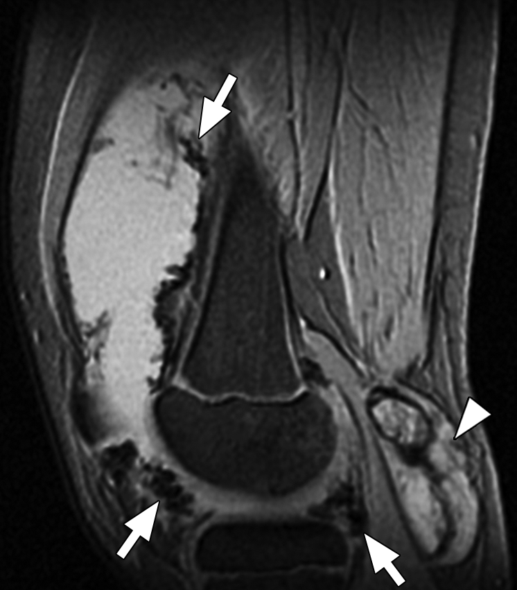
Pigmented villonodular synovitis. (a) Sagittal multiplanar GRE MR image (MPGR; GE Healthcare) (400/15; flip angle, 30°; bandwidth, 122 Hz/pixel; voxel size, 0.51 × 0.67 × 4.0 mm; FOV, 130 × 130 mm) of the knee joint shows moderate to severe joint effusion and a Baker cyst (arrowhead). Synovium shows irregular nodular thickening with dark areas of hemosiderin deposition (arrows). (b) Sagittal contrast-enhanced T1-weighted spin-echo fat-saturated MR image (Philips) (500/10; flip angle, 90°; bandwidth, 108.5 Hz/ pixel; voxel size, 0.57 × 1.1 × 4 mm; FOV, 220 × 220 mm) shows diffuse irregular enhancement of the synovium.

Figure 8b.

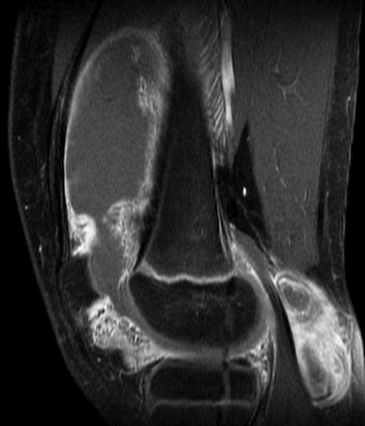
Pigmented villonodular synovitis. (a) Sagittal multiplanar GRE MR image (MPGR; GE Healthcare) (400/15; flip angle, 30°; bandwidth, 122 Hz/pixel; voxel size, 0.51 × 0.67 × 4.0 mm; FOV, 130 × 130 mm) of the knee joint shows moderate to severe joint effusion and a Baker cyst (arrowhead). Synovium shows irregular nodular thickening with dark areas of hemosiderin deposition (arrows). (b) Sagittal contrast-enhanced T1-weighted spin-echo fat-saturated MR image (Philips) (500/10; flip angle, 90°; bandwidth, 108.5 Hz/ pixel; voxel size, 0.57 × 1.1 × 4 mm; FOV, 220 × 220 mm) shows diffuse irregular enhancement of the synovium.

Figure 9a.

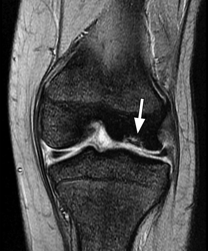
Osteochondritis dissecans. Coronal (a) and sagittal (b) T2*-weighted fast GRE MR images (T2 FFE; Philips) (695/14; flip angle, 25°; bandwidth, 108.6 Hz/pixel; voxel size, 0.58 × 0.73 × 4.0 mm; FOV, 178 × 170 mm) of the left knee joint show a lesion (arrow in a and b) of osteochondritis dissecans on the articular surface of the lateral femoral condyle. Bones are dark on T2*-weighted images because of increased susceptibility among trabeculae, while joint fluid is bright because of the long T2. This makes these sequences useful for evaluation of articular cartilage, which is seen as a structure with signal intensity intermediate between signal intensity of bones and that of joint fluid.

Figure 9b.

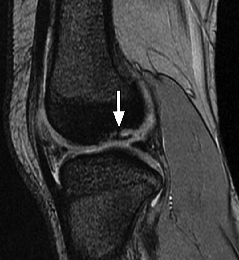
Osteochondritis dissecans. Coronal (a) and sagittal (b) T2*-weighted fast GRE MR images (T2 FFE; Philips) (695/14; flip angle, 25°; bandwidth, 108.6 Hz/pixel; voxel size, 0.58 × 0.73 × 4.0 mm; FOV, 178 × 170 mm) of the left knee joint show a lesion (arrow in a and b) of osteochondritis dissecans on the articular surface of the lateral femoral condyle. Bones are dark on T2*-weighted images because of increased susceptibility among trabeculae, while joint fluid is bright because of the long T2. This makes these sequences useful for evaluation of articular cartilage, which is seen as a structure with signal intensity intermediate between signal intensity of bones and that of joint fluid.

Susceptibility-weighted Imaging

Principles

SW imaging is an MR imaging technique that exploits the magnetic susceptibility differences of the blood, and iron and calcification in various tissues (15). SW imaging is not simply a T2*-weighted imaging approach and consists of using both magnitude and phase information (16). The phase shift present in a GRE image represents an average magnetic field of protons in a voxel, which depends on the local susceptibility of the tissues. Paramagnetic substances, such as deoxyhemoglobin, hemosiderin, and ferritin, increase the magnetic field, resulting in a positive phase relative to the surrounding parenchyma. For a left-handed (or right-handed) system, the phase is positive (or negative) when the spins precess clockwise. Diamagnetic substances, such as calcium, cause a negative phase shift. Phase images are sensitive to changes in the magnetic field caused by different components in tissues, such as deoxyhemoglobin, hematoma, or calcification, and can be used for differentiating the susceptibility differences among tissues (17). Phase itself can be a superb source of contrast, with or without T2* effects (18).

Technique

The SW imaging sequence itself is a flow-compensated, high-spatial-resolution conventional T2*-weighted sequence. The flow compensation is usually applied along all axes. The imaging parameters used at 1.5 T are as follows: 57/40; flip angle, 20°; and bandwidth, 78 Hz/pixel (19). (At higher field strengths, such as 3 T, the TE is cut in half, and the TR can be reduced accordingly.) A phase mask is created from the MR phase images, and multiplying this with the magnitude images increases the conspicuity of the smaller veins and other sources of susceptibility effects (20). Automated postprocessing gives three sets of images: phase images, magnitude images, and minimum intensity projection images (21) (Fig 10). The minimum intensity projection images represent a projection through a series of usually four sections that takes the minimum value of the signal intensity at each pixel to create an effective section of 8 mm that better shows the continuity of the veins.

Figure 10a.

Axial SW MR images obtained at 3 T (20/30; flip angle, 15°; bandwidth, 100 Hz/pixel; voxel size, 0.5 × 1.0 × 2.0 mm; FOV, 256 × 256 mm). Original magnitude image (a), original phase image (b), processed single-section magnitude image (c), and minimum intensity projection through eight sections (d) show enhancement of the veins and globi pallidi (arrowheads in b–d), which are seen as dark structures. There is also increased visibility of cortical fibers connecting adjacent sulci (arcuate fibers) (arrows in b–d), especially on phase (b) and processed magnitude (c) images. The thick (16-mm) minimum intensity projection SW image (d) shows dark vessels, with increased depiction of small veins.

Figure 10b.

Axial SW MR images obtained at 3 T (20/30; flip angle, 15°; bandwidth, 100 Hz/pixel; voxel size, 0.5 × 1.0 × 2.0 mm; FOV, 256 × 256 mm). Original magnitude image (a), original phase image (b), processed single-section magnitude image (c), and minimum intensity projection through eight sections (d) show enhancement of the veins and globi pallidi (arrowheads in b–d), which are seen as dark structures. There is also increased visibility of cortical fibers connecting adjacent sulci (arcuate fibers) (arrows in b–d), especially on phase (b) and processed magnitude (c) images. The thick (16-mm) minimum intensity projection SW image (d) shows dark vessels, with increased depiction of small veins.

Figure 10c.

Axial SW MR images obtained at 3 T (20/30; flip angle, 15°; bandwidth, 100 Hz/pixel; voxel size, 0.5 × 1.0 × 2.0 mm; FOV, 256 × 256 mm). Original magnitude image (a), original phase image (b), processed single-section magnitude image (c), and minimum intensity projection through eight sections (d) show enhancement of the veins and globi pallidi (arrowheads in b–d), which are seen as dark structures. There is also increased visibility of cortical fibers connecting adjacent sulci (arcuate fibers) (arrows in b–d), especially on phase (b) and processed magnitude (c) images. The thick (16-mm) minimum intensity projection SW image (d) shows dark vessels, with increased depiction of small veins.

Figure 10d.

Axial SW MR images obtained at 3 T (20/30; flip angle, 15°; bandwidth, 100 Hz/pixel; voxel size, 0.5 × 1.0 × 2.0 mm; FOV, 256 × 256 mm). Original magnitude image (a), original phase image (b), processed single-section magnitude image (c), and minimum intensity projection through eight sections (d) show enhancement of the veins and globi pallidi (arrowheads in b–d), which are seen as dark structures. There is also increased visibility of cortical fibers connecting adjacent sulci (arcuate fibers) (arrows in b–d), especially on phase (b) and processed magnitude (c) images. The thick (16-mm) minimum intensity projection SW image (d) shows dark vessels, with increased depiction of small veins.

Clinical Applications

SW imaging is more sensitive in detection of susceptibility effects and depicts significantly more small hemorrhagic lesions in diffuse axonal injury than does the conventional GRE sequence (P = .004) (19). Deoxyhemoglobin causes a reduction in T2*, as well as a phase difference between the vessels and surrounding parenchyma (22). Venous blood has lower T2* compared with arterial blood; hence arteries and veins can be differentiated by using a long TE. These principles are used for SW MR venography and imaging of small vessels (21). Researchers have shown that calcification can be differentiated from hemorrhage on phase images on the basis of differences in susceptibility effects (17,23,24). Increased iron deposition seen in neurodegenerative disorders such as Parkinson disease, Huntington disease, and Alzheimer disease can be better depicted with SW imaging.

Other clinical applications of SW imaging include evaluation of stroke, trauma, vasculitis, and epilepsy and characterization of brain tumors (21). Future potential uses of SW imaging include functional MR imaging, high-field-strength SW imaging, stem cell tracking, vessel wall imaging, and non–central nervous system applications such as cartilage imaging (21). More recently, researchers have shown that changes in iron content of the brain can be monitored by using SW filtered phase images (25,26). SW imaging has been shown to be of similar clinical use in both adults and children (27).

Perfusion MR Imaging

Principles

Perfusion MR imaging methods exploit signal intensity changes that occur with the passage of a tracer such as gadopentetate dimeglumine (28). As the gadolinium-based contrast agent passes in high concentration through the microvasculature, susceptibility-induced T2 and T2* relaxation occurs in surrounding tissues, which is seen as a decrease in signal intensity. The decrease in signal intensity is assumed to be linearly related to the concentration of gadolinium-based contrast agent in the microvasculature (29). The change in the signal intensity of the tissues is quantitatively related to the local concentration of gadolinium-based contrast agent and is converted into a curve of concentration versus time. By applying tracer kinetics to the concentration-time curve of the first passage of the bolus of gadolinium-based contrast agent, relative cerebral blood volume and cerebral blood flow maps are calculated (28).

Technique

Dynamic SW contrast agent–enhanced MR perfusion imaging is performed by using T2*-weighted echo-planar imaging sequences with a temporal resolution of 1–2 seconds. The T2 and/ or T2* effects outweigh the T1 effects of gadopentetate dimeglumine at high intravascular concentration. A high concentration of gadopentetate dimeglumine at first passage is achieved by injecting a dose of 0.1 mmol per kilogram of body weight with a power injector at the rate of 5 mL/ sec through an 18- or 20-gauge intravenous catheter positioned in the antecubital fossa (28).

Rapid imaging during the first pass of gadopentetate dimeglumine is performed by using a T2*-weighted echo-planar imaging sequence. This sequence can acquire 8–10 (or 16–20) sections covering the entire brain in 1 or 2 seconds. A series of 60 such multisection acquisitions is performed before, during, and after injection of gadopentetate dimeglumine. The injection of gadopentetate dimeglumine is started after the 10th run, followed by a 20-mL flush of normal saline solution at the same rate (28). Software is available that allows data analysis and calculation of various maps, such as relative cerebral blood volume, cerebral blood flow, time to peak, mean transit time, and permeability maps (Fig 11). The resolution of perfusion images is compromised to get the temporal resolution for making perfusion measurements.

Figure 11a.

Perfusion MR imaging of a patient after resection of a left parieto-occipital glioma. (a, c, d) Dynamic contrast-enhanced SW GRE echo-planar perfusion images (GRE-EPI; Siemens) (1490/40; flip angle, 90°; bandwidth, 1502 Hz/pixel; voxel size, 1.8 × 1.8 × 5.0 mm; FOV, 230 × 230 mm; echo-planar imaging factor, 128; 60 measurements) were obtained during rapid intravenous injection of gadopentetate dimeglumine. (a) Axial source image shows that all of the areas having high concentrations of gadolinium, such as arteries, are dark. (b) Graph of signal intensity versus time represents changes in signal intensity during injection of gadolinium-based contrast agent. Decrease in signal intensity between BLe and FPe lines represents first pass of contrast agent through the circulation. BLe = baseline ends, BLs = baseline starts, FPe = end of first pass. (c, d) Tracer kinetics software is applied to the curve of signal intensity versus time to obtain various color maps, where red and yellow represent high value and blue represents low value of the particular parameter. (c) Color maps show cerebral blood volume (CBV), cerebral blood flow (CBF), mean transit time (MTT), time to peak (TTP), corrected cerebral blood volume (CCBV), and permeability map (K2). (d) Separate map shows CCBV. In this case, blue (representing low flow) is seen in and around the resection cavity (arrow in c and d), which suggests that there is no viable tumor in this region. (Case courtesy of Meher Ursekar, MD, Jankharia-Piramal Imaging, Mumbai, India.)

Figure 11b.

Perfusion MR imaging of a patient after resection of a left parieto-occipital glioma. (a, c, d) Dynamic contrast-enhanced SW GRE echo-planar perfusion images (GRE-EPI; Siemens) (1490/40; flip angle, 90°; bandwidth, 1502 Hz/pixel; voxel size, 1.8 × 1.8 × 5.0 mm; FOV, 230 × 230 mm; echo-planar imaging factor, 128; 60 measurements) were obtained during rapid intravenous injection of gadopentetate dimeglumine. (a) Axial source image shows that all of the areas having high concentrations of gadolinium, such as arteries, are dark. (b) Graph of signal intensity versus time represents changes in signal intensity during injection of gadolinium-based contrast agent. Decrease in signal intensity between BLe and FPe lines represents first pass of contrast agent through the circulation. BLe = baseline ends, BLs = baseline starts, FPe = end of first pass. (c, d) Tracer kinetics software is applied to the curve of signal intensity versus time to obtain various color maps, where red and yellow represent high value and blue represents low value of the particular parameter. (c) Color maps show cerebral blood volume (CBV), cerebral blood flow (CBF), mean transit time (MTT), time to peak (TTP), corrected cerebral blood volume (CCBV), and permeability map (K2). (d) Separate map shows CCBV. In this case, blue (representing low flow) is seen in and around the resection cavity (arrow in c and d), which suggests that there is no viable tumor in this region. (Case courtesy of Meher Ursekar, MD, Jankharia-Piramal Imaging, Mumbai, India.)

Figure 11c.

Perfusion MR imaging of a patient after resection of a left parieto-occipital glioma. (a, c, d) Dynamic contrast-enhanced SW GRE echo-planar perfusion images (GRE-EPI; Siemens) (1490/40; flip angle, 90°; bandwidth, 1502 Hz/pixel; voxel size, 1.8 × 1.8 × 5.0 mm; FOV, 230 × 230 mm; echo-planar imaging factor, 128; 60 measurements) were obtained during rapid intravenous injection of gadopentetate dimeglumine. (a) Axial source image shows that all of the areas having high concentrations of gadolinium, such as arteries, are dark. (b) Graph of signal intensity versus time represents changes in signal intensity during injection of gadolinium-based contrast agent. Decrease in signal intensity between BLe and FPe lines represents first pass of contrast agent through the circulation. BLe = baseline ends, BLs = baseline starts, FPe = end of first pass. (c, d) Tracer kinetics software is applied to the curve of signal intensity versus time to obtain various color maps, where red and yellow represent high value and blue represents low value of the particular parameter. (c) Color maps show cerebral blood volume (CBV), cerebral blood flow (CBF), mean transit time (MTT), time to peak (TTP), corrected cerebral blood volume (CCBV), and permeability map (K2). (d) Separate map shows CCBV. In this case, blue (representing low flow) is seen in and around the resection cavity (arrow in c and d), which suggests that there is no viable tumor in this region. (Case courtesy of Meher Ursekar, MD, Jankharia-Piramal Imaging, Mumbai, India.)

Figure 11d.

Perfusion MR imaging of a patient after resection of a left parieto-occipital glioma. (a, c, d) Dynamic contrast-enhanced SW GRE echo-planar perfusion images (GRE-EPI; Siemens) (1490/40; flip angle, 90°; bandwidth, 1502 Hz/pixel; voxel size, 1.8 × 1.8 × 5.0 mm; FOV, 230 × 230 mm; echo-planar imaging factor, 128; 60 measurements) were obtained during rapid intravenous injection of gadopentetate dimeglumine. (a) Axial source image shows that all of the areas having high concentrations of gadolinium, such as arteries, are dark. (b) Graph of signal intensity versus time represents changes in signal intensity during injection of gadolinium-based contrast agent. Decrease in signal intensity between BLe and FPe lines represents first pass of contrast agent through the circulation. BLe = baseline ends, BLs = baseline starts, FPe = end of first pass. (c, d) Tracer kinetics software is applied to the curve of signal intensity versus time to obtain various color maps, where red and yellow represent high value and blue represents low value of the particular parameter. (c) Color maps show cerebral blood volume (CBV), cerebral blood flow (CBF), mean transit time (MTT), time to peak (TTP), corrected cerebral blood volume (CCBV), and permeability map (K2). (d) Separate map shows CCBV. In this case, blue (representing low flow) is seen in and around the resection cavity (arrow in c and d), which suggests that there is no viable tumor in this region. (Case courtesy of Meher Ursekar, MD, Jankharia-Piramal Imaging, Mumbai, India.)

Clinical Applications

Tumor growth is dependent on angiogenesis. Susceptibility-weighted MR perfusion imaging depicts microscopic capillary-level blood flow and hence serves as an indicator of angiogenesis in tumors (30,31). MR perfusion is commonly used in tumor grading (hypervascular tumors are often high grade), stereotactic biopsy guidance, monitoring response to therapy, and differentiation of radiation necrosis from recurrence (30,32–34). MR perfusion imaging is used in hyperacute stroke to determine potentially salvageable tissue in the penumbra so that appropriate action, such as intravenous or intraarterial thrombolysis, can be taken in a timely manner. Perfusion and diffusion together are the best predictors of salvageable tissue. A perfusion abnormality without a diffusion abnormality around the ischemic core indicates the penumbra of tissue that is salvageable (35). Generally, mean transit time is prolonged and relative cerebral blood flow is decreased in stroke. Relative cerebral blood volume is decreased in irreversibly injured areas and increased in spontaneous reperfusion. Other clinical applications of MR perfusion imaging include determinations of brain perfusion in moyamoya disease, vasculitis, and Alzheimer disease (36).

Functional MR Imaging

Principles

Oxyhemoglobin is diamagnetic while deoxyhemoglobin is paramagnetic relative to surrounding tissue. Deoxyhemoglobin causes a reduction in signal by creating microscopic field gradients within and around the blood vessels (37). Stimulation of a brain area causes increased cerebral blood flow in the activated region in excess of the cerebral metabolic rate of oxygen utilization. Because the local blood is more oxygenated, there is a relative decrease in deoxyhemoglobin and a slight increase in local MR signal. This phenomenon is called the blood oxygen level–dependent effect (37). The basic effect of deoxyhemoglobin causing microscopic field variation in and around the microvasculature leads to a reduction of T2* (37). The blood oxygen level–dependent effect is reduced during activation, and this leads to an increase in local T2* caused by less deoxyhemoglobin. The signal intensity change caused by the change in oxygen saturation is depicted by using a fast GRE sequence, such as echo-planar imaging, and is used to detect the area of the brain controlling a particular activity or sensation.

Technique

Functional MR imaging involves a paradigm in which the patient is asked to perform, for example, a motor activity such as finger tapping or is given visual or auditory stimuli, and the brain is then imaged with a fast T2* sensitive sequence such GRE echo-planar imaging. Paradigms include active motor, language, or cognitive tasks and passive tactile, auditory, or visual stimuli (38). The typical blood oxygen level–dependent sensitive echo-planar imaging sequence is used with the following parameters: 4000/50; flip angle, 90°; bandwidth, 2604 Hz/pixel; echo spacing, 0.47 msec; echo-planar imaging factor, 64; and matrix, 64 × 64. Data are averaged to improve the signal intensity. Statistical processing is performed to convert signal intensity change into color maps that are overlaid onto anatomic images (Fig 12). Activation indicates the location of eloquent cortex.

Figure 12.

Axial composite image in a healthy person. Functional MR imaging was performed at 3 T (Philips) (2000/30; flip angle, 90°; bandwidth, 49.2 Hz/pixel; echo-planar imaging factor, 47; voxel size, 3 × 3 × 4 mm; FOV, 230 × 230 mm). Signal change from increased local T2* caused by less deoxyhemoglobin during activation was converted into a color map by using statistical processing. This color map was overlaid onto the anatomic image to produce the composite image. This axial composite image shows blood oxygen level–dependent activation in the right hand’s motor area (yellow) and the left hand’s motor area (blue) from a boxcar experiment of alternating left and right finger tapping.

Clinical Applications

Functional MR imaging is used to map brain function and eloquent cortex in relationship to intracranial tumors, seizure foci, or vascular malformations. Eloquent cortex can get displaced or disorganized by these pathologic processes, and mapping with functional MR imaging helps to determine and potentially minimize the risk for performing surgical excision (38,39). Functional MR imaging is also used to determine the need for intraoperative mapping during excision and to select the optimal surgical approach to a lesion (31).

Iron Overload Imaging

Principles

The interaction between high-molecular-weight iron complexes, such as ferritin and hemosiderin, and water molecules leads to faster dephasing of transverse magnetization (ie, reduced T2 and T2*) in iron-laden tissues (40). This is seen as a loss of signal intensity in the tissue. This darkening of the tissue is proportional to the iron concentration (41). The longer the TE, the darker the area on the resultant image. As expected, GRE sequences are more sensitive to this inhomogeneity-induced dephasing and are more sensitive to depiction and quantification of the degree of iron overload (42).

Techniques

Two broad groups of techniques used for iron estimation are the signal intensity ratio method and the relaxometry method (43). Both of these methods can use spin-echo and/or GRE sequences.

Signal Intensity Ratio.—

In the signal intensity ratio method, the signal intensity of the target organ, such as the liver or heart, is divided by the signal intensity of a reference tissue, such as muscle or fat, by drawing a region of interest. The most commonly used protocol is that of Gandon et al (44) from the University of Rennes (Rennes, France) and includes four GRE sequences with different TEs (T1-weighted, intermediate-weighted, T2-weighted, and long-TE T2-weighted) and one T1-weighted spin-echo sequence. Signal intensity measurements from each of these sequences are used to calculate iron concentration (45).

Relaxometry.—

Signal intensity loss in the image from dephasing of transverse magnetization follows a pattern similar to radioactive decay (41). Hence, iron-mediated darkening can be characterized by time constants such as T2 or T2* or by relaxation rates such R2 (1/T2) and R2* (1/T2*). Relaxometry methods include calculation of T2 or R2 (spin-echo sequence) and T2* or R2* (GRE sequence) by acquiring multiple images at different TEs.

The most commonly used spin-echo method (TEs usually 3–18 msec) for calculation of R2 of liver was developed by St. Pierre et al (46) and is marketed as FerriScan (ResonanceHealth, Claremont, Australia) (www.ferriscan.com). Liver R2 demonstrates a curvilinear relationship with the amount of iron determined by using liver biopsy (41).

A relaxometry method to calculate hepatic and myocardial T2*, developed by Anderson et al (47), includes acquisition of GRE images with eight different TEs (2.2–20.1 msec) for liver (Fig 13) and nine different TEs (5.6–17.6 msec) for the heart. With this technique, as the myocardial iron content increases, there is a progressive decrease in ejection fraction. All patients with ventricular dysfunction had a myocardial T2* of less than 20 msec (47). The liver R2*–tracked liver iron content rises linearly with iron concentration determined by using liver biopsy (41).

Figure 13a.

Iron overload imaging of the upper portion of the abdomen. Axial T2*-weighted GRE MR images (Siemens) (500/2.4–30; flip angle, 60°; bandwidth, 380 Hz/pixel; voxel size, 1.4 × 1.0 × 6.0 mm; FOV, 400 × 400 mm) acquired with TEs of 2.4 msec (a), 5.2 msec (b), 8.0 msec (c), and 10.8 msec (d) show progressive darkening of the liver with increasing TE, which is suggestive of iron overload.

Figure 13b.

Iron overload imaging of the upper portion of the abdomen. Axial T2*-weighted GRE MR images (Siemens) (500/2.4–30; flip angle, 60°; bandwidth, 380 Hz/pixel; voxel size, 1.4 × 1.0 × 6.0 mm; FOV, 400 × 400 mm) acquired with TEs of 2.4 msec (a), 5.2 msec (b), 8.0 msec (c), and 10.8 msec (d) show progressive darkening of the liver with increasing TE, which is suggestive of iron overload.

Figure 13c.

Iron overload imaging of the upper portion of the abdomen. Axial T2*-weighted GRE MR images (Siemens) (500/2.4–30; flip angle, 60°; bandwidth, 380 Hz/pixel; voxel size, 1.4 × 1.0 × 6.0 mm; FOV, 400 × 400 mm) acquired with TEs of 2.4 msec (a), 5.2 msec (b), 8.0 msec (c), and 10.8 msec (d) show progressive darkening of the liver with increasing TE, which is suggestive of iron overload.

Figure 13d.

Iron overload imaging of the upper portion of the abdomen. Axial T2*-weighted GRE MR images (Siemens) (500/2.4–30; flip angle, 60°; bandwidth, 380 Hz/pixel; voxel size, 1.4 × 1.0 × 6.0 mm; FOV, 400 × 400 mm) acquired with TEs of 2.4 msec (a), 5.2 msec (b), 8.0 msec (c), and 10.8 msec (d) show progressive darkening of the liver with increasing TE, which is suggestive of iron overload.

Signal intensity ratio methods are faster than relaxometry methods but lack a wide range of iron content assessment and are less precise (43). Iron quantification methods that use R2* are faster compared with those that use R2 but have more susceptibility artifacts. R2* methods are more sensitive to low iron content.

Clinical Applications

MR imaging can be used to detect and quantify excess iron deposition in various organs such as the liver, heart, spleen, pancreas, and pituitary gland. Iron overload can be caused by disorders of iron absorption, such as hereditary hemochromatosis and thalassemia intermedia, defects in heme metabolism, or long-term transfusion therapy (41). Iron is toxic to the tissues and can cause endocrine, cardiac, and hepatic dysfunction. Iron overload is treated with phlebotomy or iron chelation therapy. For proper institution of these treatments, for monitoring, and for determining response, quantification of iron content is important. Traditionally, this quantification has been indirectly done by using the serum ferritin level and has been done directly by using liver biopsy. However, liver biopsy is invasive, and ferritin measurements are poorly correlated with organ iron stores, especially in the heart (47). MR imaging is a new noninvasive way to quantify the iron overload in various organs, and initial correlations are encouraging.

Conclusions

T2* relaxation, seen in GRE sequences, is decay of transverse magnetization caused by a combination of spin-spin relaxation and magnetic field inhomogeneity. Susceptibility effects cause faster T2* relaxation and lead to reduction in signal. GRE sequences can be made T2* weighted by using a low flip angle, long TE, and long TR. GRE sequences with T2*-based contrast are used to depict hemorrhage, calcification, and iron deposition in various tissues and lesions. T2*-based contrast forms the basis for higher applications such as SW imaging, perfusion MR imaging, functional MR imaging, and iron overload imaging.

References

- 1.Mugler JP., III Basic principles. In: Edelman RR, Hesselink JR, Zlatkin MB, Crues JV, eds. Clinical magnetic resonance imaging 3rd ed Philadelphia, Pa: Saunders Elsevier, 2006; 23–57 [Google Scholar]
- 2.Nitz WR, Reimer P. Contrast mechanisms in MR imaging. Eur Radiol 1999;9:1032–1046 [DOI] [PubMed] [Google Scholar]
- 3.Hendrick RE. Image contrast and noise. In: Stark DD, Bradley WG, eds. Magnetic resonance imaging 3rd ed St Louis, Mo: Mosby, 1999; 43–68 [Google Scholar]
- 4.Haacke EM, Tkach JA, Parrish TB. Reduction of T2* dephasing in gradient field-echo imaging. Radiology 1989;170:457–462 [DOI] [PubMed] [Google Scholar]
- 5.Frahm J, Haenicke W. Rapid scan techniques. In: Stark DD, Bradley WG, eds. Magnetic resonance imaging 3rd ed St Louis, Mo: Mosby, 1999; 87–124 [Google Scholar]
- 6.Chavhan GB, Babyn PS, Jankharia BG, Cheng HL, Shroff MM. Steady-state MR imaging sequences: physics, classification, and clinical applications. RadioGraphics 2008;28:1147–1160 [DOI] [PubMed] [Google Scholar]
- 7.Edelman RR, Dunkle EE, Wei Li, Kissinger KV, Thangaraj K. Practical considerations and image optimization. In: Edelman RR, Hesselink JR, Zlatkin MB, Crues JV, eds. Clinical magnetic resonance imaging 3rd ed Philadelphia, Pa: Saunders Elsevier, 2006; 58–104 [Google Scholar]
- 8.Elster AD. Gradient-echo MR imaging: techniques and acronyms. Radiology 1993;186:1–8 [DOI] [PubMed] [Google Scholar]
- 9.Tsushima Y, Endo K. Hypointensities in the brain on T2*-weighted gradient-echo magnetic resonance imaging. Curr Probl Diagn Radiol 2006;35: 140–150 [DOI] [PubMed] [Google Scholar]
- 10.Thamburaj K, Radhakrishnan VV, Thomas B, Nair S, Menon G. Intratumoral microhemorrhages on T2*-weighted gradient-echo imaging helps differentiate vestibular schwannoma from meningioma. AJNR Am J Neuroradiol 2008;29:552–557 [DOI] [PMC free article] [PubMed] [Google Scholar]
- 11.Tosaka M, Sato N, Hirato J, et al. Assessment of hemorrhage in pituitary macroadenoma by T2*-weighted gradient-echo MR imaging. AJNR Am J Neuroradiol 2007;28:2023–2029 [DOI] [PMC free article] [PubMed] [Google Scholar]
- 12.Rovira A, Orellana P, Alvarez-Sabin J, et al. Hyper-acute ischemic stroke: middle cerebral artery susceptibility sign at echo-planar gradient-echo MR imaging. Radiology 2004;232:466–473 [DOI] [PubMed] [Google Scholar]
- 13.Ishiyama K, Hashimoto M, Izumi J, et al. Tumor-liver contrast and subjective tumor conspicuity of respiratory-triggered T2-weighted fast spin-echo sequence compared with T2*-weighted gradient recalled-echo sequence for ferucarbotran-enhanced magnetic resonance imaging of hepatic malignant tumors. J Magn Reson Imaging 2008;27:1322–1326 [DOI] [PubMed] [Google Scholar]
- 14.Tonan T, Fujimoto K, Azuma S, et al. Evaluation of small dysplastic nodules and well-differentiated hepatocellular carcinomas with ferucarbotran-enhanced MRI in a 1.0-T MRI unit: utility of T2*-weighted gradient echo sequences with an intermediate-echo time. Eur J Radiol 2007;64:133–139 [DOI] [PubMed] [Google Scholar]
- 15.Reichenbach JR, Venkatesan R, Schillinger DJ, Kido DK, Haacke EM. Small vessels in the human brain: MR venography with deoxyhemoglobin as an intrinsic contrast agent. Radiology 1997;204:272–277 [DOI] [PubMed] [Google Scholar]
- 16.Reichenbach JR, Haacke EM. High-resolution BOLD venographic imaging: a window into brain function. NMR Biomed 2001;14:453–467 [DOI] [PubMed] [Google Scholar]
- 17.Yamada N, Imakita S, Sakuma T, Takamiya M. Intracranial calcification on gradient-echo phase image: depiction of diamagnetic susceptibility. Radiology 1996;198:171–178 [DOI] [PubMed] [Google Scholar]
- 18.Haacke EM, Xu Y, Cheng YC, Reichenbach JR. Susceptibility weighted imaging (SWI). Magn Reson Med 2004;52:612–618 [DOI] [PubMed] [Google Scholar]
- 19.Tong KA, Ashwal S, Holshouser BA, et al. Hemorrhagic shearing lesions in children and adolescents with posttraumatic diffuse axonal injury: improved detection and initial results. Radiology 2003;227: 332–339 [DOI] [PubMed] [Google Scholar]
- 20.Sehgal V, Delproposto Z, Haacke EM, et al. Clinical applications of neuroimaging with susceptibility-weighted imaging. J Magn Reson Imaging 2005;22: 439–450 [DOI] [PubMed] [Google Scholar]
- 21.Thomas B, Somasundaram S, Thamburaj K, et al. Clinical applications of susceptibility weighted MR imaging of the brain: a pictorial review. Neuroradiology 2008;50:105–116 [DOI] [PubMed] [Google Scholar]
- 22.Li D, Waight DJ, Wang Y. In vivo correlation between blood T2* and oxygen saturation. J Magn Reson Imaging 1998;8:1236–1239 [DOI] [PubMed] [Google Scholar]
- 23.Rauscher A, Sedlacik J, Barth M, et al. Magnetic susceptibility-weighted MR phase imaging of the human brain. AJNR Am J Neuroradiol 2005;26: 736–742 [PMC free article] [PubMed] [Google Scholar]
- 24.Gupta RK, Rao SB, Rajan J, et al. Differentiation of calcification from chronic hemorrhage with corrected gradient echo phase imaging. J Comput Assist Tomogr 2001;25:698–704 [DOI] [PubMed] [Google Scholar]
- 25.Haacke EM, Cheng NY, House MJ, et al. Imaging iron stores in the brain using magnetic resonance imaging. Magn Reson Imaging 2005;23:1–25 [DOI] [PubMed] [Google Scholar]
- 26.Haacke EM, Ayaz M, Khan A, et al. Establishing a baseline phase behavior in magnetic resonance imaging to determine normal vs abnormal iron content in the brain. J Magn Reson Imaging 2007;26: 256–264 [DOI] [PubMed] [Google Scholar]
- 27.Tong KA, Ashwal S, Obenaus A, Nickerson JP, Kido D, Haacke EM. Susceptibility-weighted MR imaging: a review of clinical applications in children. AJNR Am J Neuroradiol 2008;29:9–17 [DOI] [PMC free article] [PubMed] [Google Scholar]
- 28.Cha S, Knopp EA, Johnson G, Wetzel SG, Litt AW, Zagzag D. Intracranial mass lesions: dynamic contrast-enhanced susceptibility-weighted echo-planar perfusion MR imaging. Radiology 2002;223:11–29 [DOI] [PubMed] [Google Scholar]
- 29.Alsop D. Perfusion imaging of the brain. In: Edelman RR, Hesselink JR, Zlatkin MB, Crues JV, eds. Clinical magnetic resonance imaging 3rd ed Philadelphia, Pa: Saunders Elsevier, 2006; 333–376 [Google Scholar]
- 30.Cha S. Update on brain tumor imaging: from anatomy to physiology. AJNR Am J Neuroradiol 2006;27:475–487 [PMC free article] [PubMed] [Google Scholar]
- 31.Lemort M, Canizares-Perez AC, Van der Stappen A, Kampouridis S. Progress in magnetic resonance imaging of brain tumors. Curr Opin Oncol 2007;19: 616–622 [DOI] [PubMed] [Google Scholar]
- 32.Provenzale JM, Mukundan S, Barboriak DP. Diffusion-weighted and perfusion MR imaging for brain tumor characterization and assessment of treatment response. Radiology 2006;239:632–649 [DOI] [PubMed] [Google Scholar]
- 33.Law M, Young RJ, Babb JS, et al. Gliomas: predicting time to progression or survival with cerebral blood volume measurements at dynamic susceptibility-weighted contrast-enhanced perfusion MR imaging. Radiology 2008;247:490–499 [DOI] [PMC free article] [PubMed] [Google Scholar]
- 34.Emblem KE, Scheie D, Due-Tonnessen P, et al. Histogram analysis of MR imaging-derived cerebral blood volume maps: combined glioma grading and identification of low-grade oligodendroglial subtypes. AJNR Am J Neuroradiol 2008;29:1664–1670 [DOI] [PMC free article] [PubMed] [Google Scholar]
- 35.Karonen JO, Liu Y, Vanninen RL, et al. Combined perfusion- and diffusion-weighted MR imaging in acute ischemic stroke during the 1st week: a longitudinal study. Radiology 2000;217:886–894 [DOI] [PubMed] [Google Scholar]
- 36.Rowley HA, Roberts TP. Clinical perspectives in perfusion: neuroradiologic applications. Top Magn Reson Imaging 2004;15:28–40 [DOI] [PubMed] [Google Scholar]
- 37.Uludag K, Dubowitz DJ, Buxton RB. Basic principles of functional MRI. In: Edelman RR, Hesselink JR, Zlatkin MB, Crues JV, eds. Clinical magnetic resonance imaging 3rd ed Philadelphia, Pa: Saunders Elsevier, 2006; 249–287 [Google Scholar]
- 38.Moritz C, Haughton V. Functional MR imaging: paradigms for clinical preoperative mapping. Magn Reson Imaging Clin N Am 2003;11:529–542 [DOI] [PubMed] [Google Scholar]
- 39.Petrella JR, Shah LM, Harris KM, et al. Preoperative functional MR imaging localization of language and motor areas: effect on therapeutic decision making in patients with potentially resectable brain tumors. Radiology 2006;240:793–802 [DOI] [PubMed] [Google Scholar]
- 40.Gossuin Y, Muller RN, Gillis P. Relaxation induced by ferritin: a better understanding for an improved MRI iron quantification. NMR Biomed 2004;17: 427–432 [DOI] [PubMed] [Google Scholar]
- 41.Wood JC, Ghugre N. MRI assessment of excess iron in thalassemia, sickle cell disease and other iron overload diseases. Hemoglobin 2008;32:85–96 [DOI] [PMC free article] [PubMed] [Google Scholar]
- 42.Alustiza JM, Artetxe J, Castiella A, et al. MR quantification of hepatic iron concentration. Radiology 2004;230:479–484 [DOI] [PubMed] [Google Scholar]
- 43.Argyropoulou MI, Astrakas L. MRI evaluation of tissue iron burden in patients with beta-thalassemia major. Pediatr Radiol 2007;37:1191–1200 [DOI] [PMC free article] [PubMed] [Google Scholar]
- 44.Gandon Y, Olivie D, Guyader D, et al. Non-invasive assessment of hepatic iron stores by MRI. Lancet 2004;363:357–362 [DOI] [PubMed] [Google Scholar]
- 45.Gandon Y. Hemochromatosis and MRI. Department of Medical Imaging, University Hospital of Rennes Web site; [Accessed November 1, 2008]. http://www.radio.univ-rennes1.fr/HomeEN.html. Updated June 10, 2001. [Google Scholar]
- 46.St Pierre TG, Clark RR, Chua-anusorn W, et al. Noninvasive measurement and imaging of liver iron concentrations using proton magnetic resonance. Blood 2005;105:855–861 [DOI] [PubMed] [Google Scholar]
- 47.Anderson LJ, Holden S, Davis B, et al. Cardiovascular T2-star (T2*) MR for the early diagnosis of myocardial iron overload. Eur Heart J 2001;22: 2171–2179 [DOI] [PubMed] [Google Scholar]