A Framework for Image Segmentation Using Shape Models and Kernel Space Shape Priors

Abstract

Segmentation involves separating an object from the background in a given image. The use of image information alone often leads to poor segmentation results due to the presence of noise, clutter, or occlusion. The introduction of shape priors in the geometric active contour (GAC) framework has proven to be an effective way to ameliorate some of these problems. In this work, we propose a novel segmentation method combining image information with prior shape knowledge using level sets. Following the work of Leventon et al., we propose revisiting the use of principal component analysis (PCA) to introduce prior knowledge about shapes in a more robust manner. We utilize kernel PCA (KPCA) and show that this method outperforms linear PCA by allowing only those shapes that are close enough to the training data. In our segmentation framework, shape knowledge and image information are encoded into two energy functionals entirely described in terms of shapes. This consistent description permits us to fully take advantage of the KPCA methodology and leads to promising segmentation results. In particular, our shape-driven segmentation technique allows for the simultaneous encoding of multiple types of shapes and offers a convincing level of robustness with respect to noise, occlusions, or smearing.

1 Introduction

SEGMENTATION consists of extracting an object from an image, a ubiquitous task in computer vision applications. It is quite useful in applications ranging from finding special features in medical images to tracking deformable objects; see [1], [2], [3], [4], and the references therein. The active contour methodology has proven to be very effective for performing this task. However, the use of image information alone often leads to poor segmentation results in the presence of noise, clutter, or occlusion. The introduction of shape priors in the contour evolution process has been shown to be an effective way to address this issue, leading to more robust segmentation performances.

A number of methods that use a parameterized or an explicit representation for contours have been proposed [5], [6], [7] for active contour segmentation. In [8], the authors use the B-spline parameterization to build shape models in the kernel space [9]. The distribution of shapes in kernel space was assumed to be Gaussian and a Mahalanobis distance was minimized during the segmentation process to provide a shape prior.

The geometric active contour (GAC) framework (see [10] and the references therein) involves a parameter-free representation of contours, that is, a contour is represented implicitly by the zero level set of a higher dimensional function, typically a signed distance function [11]. In [1], the authors obtain the shape statistics by performing linear principal component analysis (PCA) on a training set of signed distance functions (SDFs). This approach was shown to be able to convincingly capture small variations in the shape of an object. It inspired other schemes to obtain the shape prior described in [2], [12], notably where SDFs were used to learn the shape variations.

However, when the object considered for learning undergoes complex or nonlinear deformations, linear PCA can lead to unrealistic shape priors by allowing linear combinations of the learned shapes that are unfaithful to the true shape of the object. Cremers et al. [13] successfully pioneered the use of kernel methods to address this issue within the GAC framework using a Parzen estimator to model the shape distribution in kernel space.

The present work builds on the methods and results outlined by the authors in [14]. We propose using kernel PCA (KPCA) to introduce shape priors for GACs. KPCA was proposed by Mika et al. [9] and allows one to combine the precision of kernel methods with the reduction of dimension in training sets. This is the first time, to our knowledge, that KPCA has been explicitly used to introduce shape priors in the GAC framework. We also propose a novel intensity-based segmentation method specifically tailored to meaningfully allow for the inclusion of a shape prior. Image and shape information are described in a consistent fashion that allows us to combine energies to realize meaningful trade-offs.

We now outline the contents of this paper. In Section 2, we briefly recall generalities concerning active contours using level sets. In Section 3, we propose a consistent method to introduce shape priors within the GAC framework, using linear PCA and KPCA. Next, in Section 4, we propose a novel intensity-based energy functional separating an object from the background in an image. This energy functional has a strong shape interpretation. Then, in Section 5, we present a robust segmentation framework, combining image cues and shape knowledge in a consistent fashion. The performances of linear PCA and KPCA are compared and the performance and robustness of our segmentation method are demonstrated on various challenging examples in Section 6. Finally, in Section 7, we make our conclusions and describe possible future research directions.

2 Level-Set Evolution

Level-set representations were introduced by Osher and Sethian [15], [16] to model interface motion and became a popular tool in the fields of image processing and computer vision. The idea consists of representing a contour by the zero-level set of a smooth Lipschitz continuous function. A common choice is to use an SDF for embedding the contour. The contour is propagated implicitly by evolving the embedding function to decrease a chosen energy functional. Implicit representations present the advantage of avoiding dealing with complex resampling schemes of control points. Moreover, the contour represented implicitly can naturally undergo topological changes such as splitting and merging.

In what follows, the SDF representing the contour of interest will be denoted by ϕ. The SDF ϕ is a function ϕ : Ω↦R and the contour corresponds to the zero-level set of ϕ, that is, {(x, y) ∈ Ω/ϕ(x, y) = 0}. The convention ϕ(x, y) ≥ 0 will be taken for points (x, y) belonging to the interior of the contour.

Typically, the energy functional is minimized via a gradient descent approach. Accordingly, one defines an energy functional in terms of ϕ, namely, E(ϕ) (see, for example, [17], [16], [15], and references therein), and, then, the contour evolution is derived via the following gradient descent flow:

$$\frac{d\varphi }{dt}=-{\nabla }_{\varphi }E.$$ (1)

This amounts to deforming the contour from an initial contour ϕ₀ in order to minimize the energy E(ϕ).

3 Linear and Kernel PCA for Shape Priors

In this section, we recall a general formulation allowing one to perform linear PCA, as well as KPCA, on any data set [18], [19]. Then, we present specific kernels allowing us to perform linear or nonlinear PCA on training sets of shapes. Finally, we propose an energy functional allowing us to introduce shape priors obtained from either linear PCA or KPCA within the GAC framework. Recent studies compared other methods such as locally linear embedding (LLE) or kernel LLE to perform shape analysis and learning (with better results usually observed on the tested sequences for kernel LLE as compared to LLE; see [20]). Comparable levels of performance were observed for KPCA and for kernel LLE. Although the present framework is general enough to use other learning methods, we focus on KPCA in what follows.

3.1 KPCA

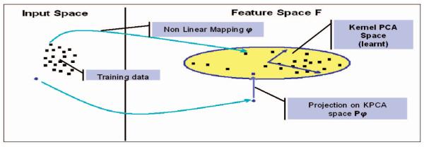
KPCA can be considered to be a generalization of linear PCA. This technique was introduced by Mika et al. [9] and has proven to be a powerful method to extract nonlinear structures from a data set. The idea behind KPCA consists of mapping a data set from an input space $\mathcal{I}$ into a feature space F via a nonlinear function φ. Then, PCA is performed in F to find the orthogonal directions (principal components) corresponding to the largest variation in the mapped data set. The first l principal components account for as much of the variance in the data as possible by using l directions. In addition, the error in representing any of the elements of the training set by its projection onto the first l principal components is minimal in the least squares sense.

The nonlinear map $\phi :\mathcal{I}\to F$ typically does not need to be known through the use of Mercer kernels. A Mercer kernel is a function k(·, ·) such that, for all data points χ_i, the kernel matrix K(i, j) = k(χ_i, χ_j) is symmetric positive definite [9]. According to Mercer’s Theorem (see [21]), computing k(·, ·) as a function of $\mathcal{I}\times \mathcal{I}$ amounts to computing the inner scalar product in F : k(χ_a, χ_b) = (φ(χ_a) · φ(χ_b)), with $({\chi }_a,{\chi }_b)\in \mathcal{I}\times \mathcal{I}$. This scalar product in F defines a distance d_F such as

$$\begin{array}{cc}\hfill d_F^2\left(\phi \right({\chi }_a),\phi ({\chi }_b\left)\right)& ={\Vert \phi \left({\chi }_a\right)-\phi \left({\chi }_b\right)\Vert }^2\hfill \\ \hfill & =k({\chi }_a,{\chi }_a)-2k({\chi }_a,{\chi }_b)+k({\chi }_b,{\chi }_b).\hfill \end{array}$$

We now briefly describe the KPCA method [9]. Let τ = {χ₁, χ₂, …, χ_N} be a set of training data. The centered kernel matrix $\tilde{\mathbf{K}}$ corresponding to τ is defined as

$$\begin{array}{cc}\hfill \tilde{\mathbf{K}}& =\left(\left(\phi \right({\chi }_i)-\stackrel{‒}{\phi })\cdot \left(\phi \right({\chi }_j)-\stackrel{‒}{\phi })\right)\hfill \\ \hfill & =\left(\tilde{\phi }\right({\chi }_i)\cdot \tilde{\phi }({\chi }_j\left)\right)=\tilde{k}({\chi }_i,{\chi }_j),\text{for}i\in [\mid 1,N\mid ],\hfill \end{array}$$ (2)

with $\stackrel{‒}{\phi }=\frac{1}{N}{\sum }_{i=1}^N\phi \left({\chi }_i\right)$, $\tilde{\phi }\left({\chi }_i\right)=\phi \left({\chi }_i\right)-\stackrel{‒}{\phi }$ being the centered map corresponding to χ_i and $\tilde{k}(.,.)$ denoting the centered kernel function. Since $\tilde{\mathbf{K}}$ is symmetric, it can be decomposed as

$$\tilde{\mathbf{K}}=\mathbf{U}\mathbf{S}{\mathbf{U}}^t,$$ (3)

where S = diag(γ₁, …, γ_N) is a diagonal matrix containing the eigenvalues of $\tilde{\mathbf{K}}$. U = [u₁, …, u_N] is an orthonormal matrix. The column vectors u_i = [u_i1, …, u_iN]^t are the eigenvectors corresponding to the eigenvalues γ_is. Besides, it can easily be shown that $\tilde{\mathbf{K}}=\mathbf{H}\mathbf{K}\mathbf{H}$, where $\mathbf{H}=\mathbf{I}-\frac{1}{N}{11}^t$. 1 = [1, …, 1]^t is an N × 1 vector.

Let C denote the covariance matrix of the elements of the training set mapped by $\tilde{\phi }$. Within the KPCA methodology, the covariance matrix C, which is possibly of very high dimension, does not need to be computed explicitly. Only $\tilde{\mathbf{K}}$ needs to be known to extract features from the training set since the eigenvectors of C are simple functions of the eigenvectors of $\tilde{\mathbf{K}}$ [18]. The subspace of the feature space F spanned by the first l eigenvectors of C will be referred to as the KPCA space in what follows: The KPCA space is the subspace of F obtained from learning the training data.

Let χ be any element of the input space $\mathcal{I}$. The projection of χ on the KPCA space will be denoted by P^lφ(χ).¹ The projection P^lφ(χ) can be obtained as described in [9]. The squared distance $d_F^2$ between a test point χ mapped by φ and its projection on the KPCA space is given by

$$\begin{array}{cc}\hfill & d_F^2\left[\phi \right(\chi ),P^l\phi (\chi \left)\right]={\Vert \phi \left(\chi \right)-P^l\left(\chi \right)\Vert }^2,\hfill \\ \hfill & =k(\chi ,\chi )-2\left(\phi \right(\chi ).P^l\phi (\chi \left)\right)+\left(P^l\phi \right(\chi )\cdot P^l\phi (\chi \left)\right).\hfill \end{array}$$

This distance measures the discrepancy between a (mapped) element of $\mathcal{I}$ and the elements of the learned space and will be minimized to introduce shape knowledge in the contour evolution process in Section 3.3. Using some matrix manipulations, this squared distance can be expressed only in terms of kernels as

$$\begin{array}{cc}\hfill & d_F^2\left[\phi \right(\chi ),P^l\phi (\chi \left)\right]=\hfill \\ \hfill & k(\chi ,\chi )+\frac{1}{N^2}{1}^t\mathbf{K}1-\frac{2}{N}{1}^t{\mathbf{k}}_{\chi }+{\tilde{\mathbf{k}}}_{\chi }^t\mathbf{M}\tilde{\mathbf{K}}\mathbf{M}{\tilde{\mathbf{k}}}_{\chi }-2{\tilde{\mathbf{k}}}_{\chi }^t\mathbf{M}{\tilde{\mathbf{k}}}_{\chi },\hfill \end{array}$$ (4)

where k_χ = [k(χ,χ₁) k(χ,χ₂), …, k(χ,χ_N)]^t, ${\tilde{\mathbf{k}}}_{\chi }=\mathbf{H}({\mathbf{k}}_{\chi }-\frac{1}{N}\mathbf{K}1)$ and $\mathbf{M}={\sum }_{i=1}^l\frac{1}{{\gamma }_i}{\mathbf{u}}_i{\mathbf{u}}_i^t$.

Fig. 1 recapitulates the KPCA methodology, as well as the projection operation on the learned space.

Fig. 1.

Kernel PCA methodology. A training set is mapped from input space $\mathcal{I}$ to feature space F via a nonlinear function φ. PCA is performed in F to determine the principal directions defining the kernel PCA space (learned space): oval area. Any element of $\mathcal{I}$ can then be mapped to F and projected on the kernel PCA space via P^lφ.

3.2 Kernels for Linear and Nonlinear PCA

3.2.1 Linear PCA

In [1], a method is presented to learn shape variations by performing PCA on a training set of shapes (closed curves) represented as the zero level sets of SDFs. Using the following kernel in the formulation of the KPCA presented above amounts to performing linear PCA on the given SDFs:

$$k_{id}({\varphi }_i,{\varphi }_j)=({\varphi }_i.{\varphi }_j)=\int \int {\varphi }_i(u,v){\varphi }_j(u,v)du.dv$$ (5)

for all SDFs ϕ_i and ϕ_j : R² → R. The subscript id stands for the identity function: When performing linear PCA, the kernel used is the inner scalar product in the input space; hence, the corresponding mapping function φ = id.

A different representation for shapes is based on the use of binary maps, that is, one sets to 1 the pixels located inside the shape and to 0 the pixels located outside (see Fig. 4).

Fig. 4.

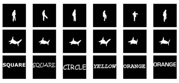
Three training sets (before alignment—binary images are presented here). First row: “Soccer Player” silhouettes (6 of the 22 used). Second row: “Shark” silhouettes (6 of the 15 used). Third row: “4 Words” (6 of the 80 learned).

One can change the shape representation from SDFs to binary maps using the Heaviside function

$$H\left(\varphi \right)=H\varphi =\{\begin{array}{cc}1\hfill & \text{if}\varphi \ge 0,\hfill \\ 0\hfill & \text{else}.\hfill \end{array}\phantom{\}}$$

Note that, in this case, the kernel allowing one to perform linear PCA is given by

$$k_{id}(H{\varphi }_i,H{\varphi }_j)=H(H{\varphi }_i.H{\varphi }_j).$$ (6)

In numerical applications, a smooth version H_∊ϕ of Hϕ can be obtained by taking $H_{∊}\varphi =\frac{1}{2}+\frac{1}{\pi }\arctan \left(\frac{\varphi }{∊}\right)$ for ∊ small. The derivative of H will be noted δ in the rest of this paper. In numerical applications, a smooth version δ_∊ϕ of δϕ can be obtained by taking ${\delta }_{∊}\varphi =\frac{1}{\pi }\frac{1}{1+{\left(\frac{\varphi }{∊}\right)}^2}$.

3.2.2 Nonlinear PCA

Choosing a nonlinear kernel function k(·, ·) is the basis of nonlinear PCA. The exponential kernel has been a popular choice in the machine learning community and has proven to nicely extract nonlinear structures from data sets; see, for example, [19]. Using SDFs for representing shapes, this kernel is given by

$$k_{{\phi }_{\sigma }}({\varphi }_i,{\varphi }_j)=e^{\frac{-{\Vert {\varphi }_i-{\varphi }_j\Vert }^2}{2{\sigma }^2}},$$ (7)

where σ² is a variance parameter estimated a priori and ∥ϕ_i − ϕ_j∥² is the squared (L₂-distance between two SDFs ϕ_i and ϕ_j. The subscript φ_σ stands for the nonlinear mapping corresponding to the exponential kernel; this mapping also depends on the choice of ϕ. If the shapes are represented by binary maps, the corresponding kernel is

$$k_{{\phi }_{\sigma }}(H{\varphi }_i,H{\varphi }_j)=e^{\frac{-{\Vert H{\varphi }_i-H{\varphi }_j\Vert }^2}{2{\sigma }^2}}.$$ (8)

This exponential kernel is one among many possible choices of Mercer kernels. Other kernels may be used to extract other specific features from the training set; see [9].

3.3 Shape Prior for GAC

In order to include prior shape knowledge in the GAC framework, we propose using the projection on the KPCA space as a model and minimizing the following energy functional:

$$E_{\text{shape}}^{\mathrm{F}}\left(\chi \right)≔d_F^2\left[\phi \right(\chi ),P^l\phi (\chi \left)\right].$$ (9)

The superscript F in $E_{\text{shape}}^{\mathrm{F}}$ denotes the fact that the shape knowledge is expressed as a distance in feature space. A similar idea was presented in [22] for the purpose of pattern recognition and denoising. In (9), χ is a test shape represented using either an SDF (χ = ϕ) or a binary map (χ = Hϕ) and φ refers to either id (linear PCA) or φ_σ (KPCA). Minimizing $E_{\text{shape}}^{\mathrm{F}}$ as in (1) amounts to driving the test shape χ toward the KPCA space computed a priori from a training set of shapes using (3). This contour evolution involving only the minimization of $E_{\text{shape}}^{\mathrm{F}}$ (no image information) will be referred to as “warping” in what follows.

A number of researchers have proposed minimizing the distance between the current shape and the mean shape obtained from a training set. The assumption is indeed often made that the underlying distribution of familiar “shapes,” in either the input or feature space is Gaussian [1], [7], [8]. Following this assumption, driving the curve toward the mean shape is a sensitive choice. Here, however, we deliberately chose to use the projection of the (mapped) current SDF to drive the evolution because we would like to deal with objects of different geometry in the training set (see, for example, Fig. 4c; a training set of four words was used for the experiments). When dealing with objects of very different shapes, the underlying distribution can be quite non-Gaussian (for example, multimodal).

Thus, the average shape would not be meaningful in this case since it would amount to mixing shapes belonging to different clusters. As a consequence, driving the (mapped) current shape toward its projection on the KPCA space appears to be a more sensible choice for our purposes. In addition, choosing the projection as a model of shape allows for comparing the given learning methods without image information, that is, by warping the same initial contour for each method and comparing the final results in terms of their resemblance to the elements of the training set. The final shape obtained can be interpreted as “the most probable shape of the initial contour given what is known from the data” (see the warping experiments in Section 6.2). If the mean shape is chosen as a shape model, warping would result in the initial contour converging to this mean shape and no comparison would be possible among learning methods. Thus, in this latest case, image information must be included and it is difficult to conclude whether differences between segmentation results are due to differences in the performances of the learning methods or simply to poor balancing between image and shape information.

The gradient of E_shape can be computed by applying the calculus of variations on (9), using the expression of $d_F^2\left(\phi \right(\xi ),P^l\phi (\xi \left)\right)$ in (4). The energy $E_{\text{shape}}^{\mathrm{F}}\left(\chi \right)$ can be minimized as follows:

$$\frac{d\varphi }{dt}=-{\nabla }_{\varphi }{E}_{\text{shape}}^{\mathrm{F}}=-{\nabla }_{\chi }{E}_{\text{shape}}^{\mathrm{F}}.\frac{d\chi }{d\varphi }.$$ (10)

The minimization of E_shape for any arbitrary contour (no image information) results in the deformation of the contour toward a familiar shape (as presented in Section 6.2).

For the exponential kernel involving SDFs and given in (7), the following result is obtained:

$${\nabla }_{\varphi }{E}_{\text{shape}}^{\mathrm{F}}=-\frac{{\Sigma }_{i=1}^N{g}_i\left(\varphi \right).k_{{\phi }_{\sigma }}(\varphi ,{\varphi }_i).[\varphi -{\varphi }_i]}{{\sigma }^2}$$ (11)

with $\left[g_1\right(\varphi ),\dots ,g_N(\varphi \left)\right]=-\frac{2}{N}{1}^t+2{\tilde{\mathbf{k}}}_{\varphi }^t\mathbf{M}\tilde{\mathbf{K}}\mathbf{M}\mathbf{H}-4{\tilde{\mathbf{k}}}_{\varphi }^t\mathbf{M}\mathbf{H}$ and ${\tilde{\mathbf{k}}}_{\varphi }$, M, and $\tilde{\mathbf{K}}$ computed for k_φσ.

For the exponential kernel involving binary maps and given in (8), one derives that

$${\nabla }_{\varphi }{E}_{\text{shape}}^{\mathrm{F}}=-\frac{{\Sigma }_{i=1}^N{g}_i\left(\varphi \right).k_{{\phi }_{\sigma }}(H\varphi ,H{\varphi }_i).\delta \varphi .[H\varphi -H{\varphi }_i]}{{\sigma }^2},$$ (12)

where ${\tilde{\mathbf{k}}}_{\varphi }$, M, and $\tilde{\mathbf{K}}$ are computed for the kernel k_φσ(H., H.).

For the kernel given in (5), corresponding to linear PCA on SDFs, the following result is obtained:

$${\nabla }_{\varphi }{E}_{\text{shape}}^{\text{linear}}=2\varphi +{\Sigma }_{i=1}^N{g}_i\left(\varphi \right).{\varphi }_i,$$ (13)

where ${\tilde{\mathbf{k}}}_{\varphi }$, M, and $\tilde{\mathbf{K}}$ are computed for the kernel k_id.

Finally, for the kernel given in (6), corresponding to linear PCA on binary maps, one finds that

$${\nabla }_{\varphi }{E}_{\text{shape}}^{\text{linear}}=2\delta \varphi +{\Sigma }_{i=1}^N{g}_i\left(H\varphi \right).H{\varphi }_i.\delta \varphi ,$$ (14)

where ${\tilde{\mathbf{k}}}_{\varphi }$, M, and $\tilde{\mathbf{K}}$ are computed for the kernel k_id(H., H.).

4 Intensity-Based Segmentation

Different models [23], [24], [25], [26], [27] which incorporate geometric and/or photometric (color, texture, intensity) information have been proposed to perform region-based segmentation using level sets. Other methods such as those in [28], [29] use local information, that is, edges. Most of the region-based models have been inspired by the region competition technique proposed in [30] and usually offer a higher level of robustness to noise than models based on local information. Morel and Solimini’s book [31] is a nice reference on the various variational segmentation methods.

We now formulate our region-based segmentation approach aimed at separating an object from the background in a given image I. As with most region-based approaches, we assume that the object and background are characterized by statistical properties which are visually consistent and distinct from each other. The main idea behind the proposed method is to build an “image-shape model” (denoted by G_[I,ϕ(t)]) by extracting a binary map from the image I, based on the estimates of the intensity statistics of the object (and background) available at each step t of the contour evolution.

Let P_in(I(x, y)) = p(I(x, y)|(x, y) ∈) Inside denote the probability of the image intensity the taking the value I(x, y), knowing that (x, y) belongs to the interior of the contour. Similarly, let P_out(I(x, y)) = p(I(x, y)|(x, y) ∈) Outside) denote the probability of the image intensity taking the value I(x, y), belongs to the exterior of the contour.² Estimates of these probabilities can be computed from the image intensities corresponding to pixels inside and outside the contour at each step t of the contour evolution. This will be detailed further in Sections 4.1 and 4.2. Given a meaningful initialization of the evolving curve, these statistics provide valuable information about the statistics of the object and the background. Intuitively, the conditional densities P_in and P_out are, respectively, the best available estimates of the unknown conditional densities P_O = p((x, y) ∈ Object|I(x, y)) (density the pixel intensities belonging to the object) and P_B = p((x, y) ∈ Background|I(x, y)) (density of the pixel intensities belonging to the background). The image-shape model G[I,ϕ(t)] is built in the following manner:

$$G_{[I,\varphi (t\left)\right]}(x,y)=\{\begin{array}{cc}1\hfill & \text{if}{P}_{\text{in}}\left(I\right(x,y\left)\right)\ge P_{\text{out}}\left(I\right(x,y\left)\right)\hfill \\ 0\hfill & \text{if}{P}_{\text{in}}\left(I\right(x,y\left)\right)<P_{\text{out}}\left(I\right(x,y\left)\right).\hfill \end{array}\phantom{\}}$$ (15)

Hence, the image-shape model G_[I,ϕ(t)] can be interpreted as the most likely shape of the object of interest based on these statistics: Pixels set to 1 in G_[I,ϕ(t)] correspond to pixels of the image that are deemed to belong to the object of interest, while pixels set to 0 are believed to not be part of the object.

To perform image segmentation, the contour at time t is deformed toward this image-shape model by minimizing the following energy:

$$\begin{array}{cc}\hfill E_{\text{image}}(\varphi ,I):& ={\Vert H\varphi -G_{[I,\varphi (t\left)\right]}\Vert }^2,\hfill \\ \hfill & ={\int }_{\Omega }{(H\varphi -G_{[I,\varphi (t\left)\right]})}^{2}dxdy.\hfill \end{array}$$ (16)

This energy amounts to measuring the distance between two binary maps, namely, Hϕ and G_[I,ϕ(t)]. This is quite valuable in the present context, where shapes can be represented using binary maps, as in earlier sections. Thus, when the shape energy described in (9) is combined with the image energy defined in (16), all of the elements can be expressed in terms of shapes and meaningful trade-offs can be realized. The gradient of E_image can be computed, assuming that the image-shape model G_[I,ϕ(t)] undergoes little variation during one step of the contour evolution:³

$${\nabla }_{\varphi }{E}_{\text{image}}=2\delta \varphi .(H\varphi -G_{[I,\varphi (t\left)\right]}).$$ (17)

Here, the gradient “points” in the direction of the image-shape model, driving the contour toward it.

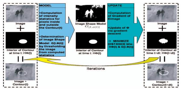
Fig. 2 offers a visualization of the proposed segmentation algorithm: First, the image-shape model is built and, then, the contour is evolved toward the shape model.

Fig. 2.

Model phase: An image-shape model is built from the statistics of the image. Update phase: The contour is evolved to reduce the distance between the shape it underlines and the image-shape model.

4.1 Object and Background with Different Mean Intensities

When the object of interest is consistently darker (or brighter) than the background, a reasonable segmentation may be obtained by considering only the mean intensities of the object and of the background; see [23] and [24]. Such images can be treated within the proposed framework by assuming that the intensities of the object and the background have a Gaussian distribution of different means and identical variances.⁴ Following this assumption, at each step t of the contour evolution, P_in(I(x, y)) and P_out(I(x, y)) can be approximated as

$$P_{\text{in}}\left(I\right(x,y\left)\right)=\beta e^{\frac{{(I-{\mu }_{\text{in}})}^2}{2{\sigma }_0^2}}\text{and}{P}_{\text{out}}\left(I\right(x,y\left)\right)=\beta e^{\frac{{(I-{\mu }_{\text{out}})}^2}{2{\sigma }_0^2}},$$ (18)

with

$${\mu }_{\text{in}}=\frac{\int I(x,y)H\varphi dxdy}{\int H\varphi dxdy},$$

respectively,

$${\mu }_{\text{out}}=\frac{\int I(x,y)(1-H\varphi )dxdy}{\int (1-H\varphi )dxdy},$$

denoting the mean intensity of the pixels located inside (respectively, outside) the contour and (σ₀, β) ∈ R × R. The optimal threshold separating the object from the background based on the knowledge of the image statistics at time t is $\frac{{\mu }_{\text{in}}+{\mu }_{\text{out}}}{2}$. Following the definition of G_[I,ϕ(t)] in (15), two cases need to be distinguished to compute the image-shape model at time t:

$$\begin{array}{cc}\hfill & \text{if}{\mu }_{\text{in}}>{\mu }_{\text{out}},G_{[I,\varphi (t\left)\right]}(x,y)=\{\begin{array}{cc}1\hfill & I(x,y)\ge \frac{{\mu }_{\text{in}}+{\mu }_{\text{out}}}{2},\hfill \\ 0\hfill & \text{else},\hfill \end{array}\phantom{\}}\hfill \\ \hfill & \text{if}{\mu }_{\text{in}}\le {\mu }_{\text{out}},G_{[I,\varphi (t\left)\right]}(x,y)=\{\begin{array}{cc}1\hfill & I(x,y)\le \frac{{\mu }_{\text{in}}+{\mu }_{\text{out}}}{2},\hfill \\ 0\hfill & \text{else}.\hfill \end{array}\phantom{\}}\hfill \end{array}$$

Notice that G_[I,ϕ(t)] is the image-shape model (binary map) obtained from thresholding the image intensities so that values closer to μ_in are classified as object (set to 1) and others are classified as background (set to 0). For numerical experiments, the function G_[I,ϕ(t)] is calculated as follows:

$$\begin{array}{cc}\hfill \text{if}\hfill & {\mu }_{\text{in}}>{\mu }_{\text{out}},\hfill \\ \hfill \hfill & G_{[I,\varphi (t),\epsilon ]}(x,y)=\frac{1}{2}+\frac{1}{\pi }\arctan \left(\frac{\frac{I(x,y)-{\mu }_{\text{in}}+{\mu }_{\text{out}}}{2}}{\epsilon }\right)\hfill \\ \hfill \text{else}\hfill & G_{[I,\varphi (t),\epsilon ]}(x,y)=\frac{1}{2}-\frac{1}{\pi }\arctan \left(\frac{\frac{I(x,y)-{\mu }_{\text{in}}+{\mu }_{\text{out}}}{2}}{\epsilon }\right),\hfill \end{array}$$

where ε is a parameter such that G_[I,ϕ(t),ε] → G_[I,ϕ(t)] as ε → 0.

4.2 Object and Background with Different Global Statistics

When the image statistics of the object of interest (or background) have more complicated distributions than the one alluded to above, a more involved scheme needs to be applied to perform segmentation. A few methods were recently presented aiming at performing segmentation using global considerations about the statistics of both the object and the background in an unsupervised fashion. For instance, in [32], contour evolution is undertaken in order to reduce the mutual information between the object and background statistics, while, in [33], the Bhattacharyya distance between the histograms of the object and background is minimized. Promising segmentation results were obtained on a wide array of objects and backgrounds having diverse intensity distributions.

The image-shape model approach presented above can be generalized to take into account the global statistics of both the image and the background. At each step t of the contour evolution, the probability density functions P_in(I(x, y)) and P_out(I(x, y)) can be estimated, using Parzen windows [34], in the following manner:

$$\begin{array}{c}\hfill P_{\text{in}}\left(I\right(x,y\left)\right)=\frac{\int K\left(I\right(x,y)-I(x^{\prime },y^{\prime }\left)\right)H\varphi (x^{\prime },y^{\prime })d{x}^{\prime }d{y}^{\prime }}{\int H\varphi (x,y)dxdy}\text{and}\hfill \\ \hfill P_{\text{out}}\left(I\right(x,y\left)\right)=\frac{\int K\left(I\right(x,y)-I(x^{\prime },y^{\prime }\left)\right)[1-H\varphi (x^{\prime },y^{\prime }\left)\right]d{x}^{\prime }d{y}^{\prime }}{\int [1-H\varphi (x,y\left)\right]dxdy},\hfill \end{array}$$

where K can be chosen to be the Gaussian kernel with zero mean and chosen variance.⁵

The image-shape model can be constructed by plugging the estimates of P_in and P_out into (15). In numerical applications, a smoothed version of G_[I,ϕ(t)] may be computed (for ε small) as

$$G_{[I,\varphi (t\left)\right]}(x,y)=\frac{1}{2}+\frac{1}{\pi }\arctan \left(\frac{P_{\text{in}}\left(I\right(x,y\left)\right)-P_{\text{out}}\left(I\right(x,y\left)\right)}{\epsilon }\right).$$

5 Combining Shape Prior and Intensity Information

5.1 Balancing Energy Functionals

In this section, we combine shape knowledge obtained by performing nonlinear PCA on binary maps with image information obtained by building an “image-shape model.” Classically, image and shape information are combined by defining a total energy E_total:

$$E_{\text{total}}(I,\varphi )=E_{\text{shape}}^{\mathrm{F}}\left(\varphi \right)+\beta .E_{\text{image}}(I,\varphi ).$$ (19)

Using Bayes’ formula, it can be shown that minimizing the above energy functional amounts to maximizing the posterior probability of the curve given current image information and shape knowledge. The coefficient β represents the level of trust given to image information (higher βs result in emphasizing image information). Considering −∇_ϕE_total in (19), two forces are obtained: One is the image force f_image = −β∇_ϕE_image, the other is the shape force $f_{\text{shape}}^{\mathrm{F}}=-{\nabla }_{\varphi }{E}_{\text{shape}}^{\mathrm{F}}$. The gradient descent process described in (1) converges to a local minimum where f_image and $f_{\text{shape}}^{\mathrm{F}}$ balance each other (same amplitude and opposite directions).

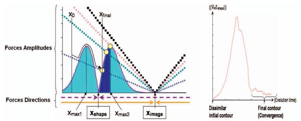
However, E_image is a squared L₂-distance in the input space, whereas $E_{\text{shape}}^{\mathrm{F}}$ is a squared distance in the feature space. As a consequence, a meaningful balance between f_image and $f_{\text{shape}}^{\mathrm{F}}$ would be hard to reach. The gradient ${\nabla }_{\varphi }{E}_{\text{shape}}^{\mathrm{F}}$ exhibits a nonlinear behavior due to the exponential terms it involves. To illustrate this point, one can consider a one-dimensional static version of E_image and $E_{\text{shape}}^{\mathrm{F}}$.⁶ Let $E_{\text{image}}^{1\mathrm{d}}={(x-x_{\text{image}})}^2$ be the one-dimensional analogous of E_image, with x_image being the one-dimensional equivalent to the image-shape model, and let $E_{\text{shape}}^{1\mathrm{d}}=2-2e^{\frac{{(x-x_{\text{shape}})}^2}{2{\sigma }^2}}$ be the one-dimensional analogous of $E_{\text{shape}}^{\mathrm{F}}$, with x_shape being the one-dimensional equivalent to the shape model obtained from learning.⁷ Although this is usually not the case during the actual evolution process, the models x_image and x_shape will be considered constant throughout this discussion for simplicity. The one-dimensional forces $f_{\text{image}}^{1\mathrm{d}}$ and $f_{\text{shape}}^{1\mathrm{d}}$ corresponding, respectively, to $E_{\text{image}}^{1\mathrm{d}}$ and $E_{\text{shape}}^{1\mathrm{d}}$ can easily be computed as

$$\begin{array}{cc}\hfill f_{\text{image}}^{1\mathrm{d}}& =-2\beta .(x-x_{\text{image}})\text{and}\hfill \\ \hfill f_{\text{shape}}^{1\mathrm{d}}& =-\frac{2}{{\sigma }^2}(x-x_{\text{shape}})e^{\frac{{(x-x_{\text{shape}})}^2}{2{\sigma }^2}}.\hfill \end{array}$$

The amplitudes and directions of $f_{\text{image}}^{1\mathrm{d}}$ and $f_{\text{shape}}^{1\mathrm{d}}$ are presented in Fig. 3 for fixed values of x_image, x_shape, and σ, as well as for different values of β. The amplitude of $f_{\text{shape}}^{1\mathrm{d}}$ presents two maxima around x_shape. The values of x, denoted x_max1 and x_max2, for which these maxima occur are x_max1 = x_shape − σ and x_max2 = x_shape + σ. During gradient descent, the variable x evolves from an initial value of x = x₀ in the direction of the force that has the highest amplitude to converge to the value of x = x_final for which $f_{\text{image}}^{1\mathrm{d}}$ and $f_{\text{shape}}^{1\mathrm{d}}$ have the same amplitudes and opposite directions. Although the results presented in Fig. 3 are dependent on the particular choice of x_image, x_shape, and β, valuable insights about the consequences of the nonlinear behavior of $E_{\text{shape}}^{\mathrm{F}}$ may be inferred:

• If β is too large, $\mid f_{\text{image}}^{1\mathrm{d}}\mid$ (■ line on the graph) is always above $\mid f_{\text{shape}}^{1\mathrm{d}}\mid$: The evolution of x is not influenced by $f_{\text{shape}}^{1\mathrm{d}}$ and x should converge to x_image. Hence, it can be expected that for too large σs, no shape knowledge will contribute at all to the contour evolution and the contour will converge to the image-shape model. This is counterintuitive since, from (19), one expects that both energies contribute to the evolution (for β ≠ 0).

• If the initial value of x is biased toward x_image, for instance, x₀ located on the right of x_image, $f_{\text{shape}}^{1\mathrm{d}}$ will not contribute to the evolution of x and convergence again occurs for x = x_image. Thus, it can be expected that the final contour will be very much dependent on initial conditions. For example, if the shape of the initial contour is biased toward the image-shape model the contour could converge toward the image-shape model and shape-knowledge information would not influence the evolution.

• The darker area under the $\mid f_{\text{shape}}^{1\mathrm{d}}\mid$ curve represents the locus of the possible final values of x realizing a trade-off between image information and the knowledge of shape. These possible final values are between x_shape and x_max2. Final results for x will thus be skewed toward the shape-knowledge model and it is not possible to reach any trade-off value located between x_max2 and x_image (for any initial value x₀). Thus, the parameter σ can be expected to have a limiting influence on the possible trade-offs realizable between image information and shape knowledge, resulting in not meaningfully balanced final contours. Ideally, only the parameter β should influence the trade-off between forces, whereas σ should be chosen based on considerations of the training data only.

Fig. 3.

(a) Theoretical forces corresponding to E_image and $E_{\text{shape}}^{\mathrm{F}}$. The double-bell-shaped curve represents $\mid f_{\text{shape}}^{1\mathrm{d}}\mid$. The two-segment curves represent $\mid f_{\text{image}}^{1\mathrm{d}}\mid$ for diverse values of β (higher absolute slopes correspond to higher βs). The respective directions of both forces are materialized by the two pairs of opposite horizontal arrows at the bottom of the figure. The darker area under the $\mid f_{\text{shape}}^{1\mathrm{d}}\mid$ curve represents the locus of possible convergence points that realize a trade-off between $\mid f_{\text{image}}^{1\mathrm{d}}\mid$ and $\mid f_{\text{shape}}^{1\mathrm{d}}\mid$: for the +, ×, and △4 lines, the corresponding possible point of convergence is indicated by a circle (no trade-off is realizable between $\mid f_{\text{image}}^{1\mathrm{d}}\mid$ and $\mid f_{\text{shape}}^{1\mathrm{d}}\mid$ for the ■ line). (b) Experimental result highlighting the nonlinear behavior of the L₂ norm of ${\nabla }_{\varphi }{E}_{\text{shape}}^{\mathrm{F}}$. An initial contour “far away” from the learned shapes was warped (note the similarity between the experimental curve and the theoretical solid-line curve in the leftmost graph).

Fig. 3b presents the typical behavior of the L₂ norm of $f_{\text{shape}}^{\mathrm{F}}$, obtained when warping an initial contour very “far from” (that is, dissimilar to) the elements of the training set, until convergence. This empirical result for the norm of $f_{\text{shape}}^{\mathrm{F}}$ exhibits very similar behavior to its one-dimensional theoretical counterpart $\mid f_{\text{shape}}^{1\mathrm{d}}\mid$, validating the remarks made above.⁸

Hence, these issues need to be addressed in order to take advantage of the KPCA technique in a robust (for example, less dependent on initial conditions), intuitive, and meaningful manner. We now proceed to explain a methodology to address the aforementioned issues for the exponential kernel (the methodology is general enough to accommodate any invertible kernel of the form k(x, y) = k(∥x − y∥)). The nonlinear behavior of $\nabla E_{\text{shape}}^{\mathrm{F}}$ stems from the fact that the energy is defined as a distance in the feature space. We would like to redefine the shape energy so that the amplitude of its gradient exhibits a linear behavior (similar to ∇E_image for which the energy is defined as a distance in the input space). We note that distances in the feature space and the input space are related as follows, for any SDFs ϕ_a and ϕ_b:

$$\begin{array}{cc}\hfill d_F^2({\varphi }_a,{\varphi }_b)& =2-2k_{{\phi }_{\sigma }}(H{\varphi }_a,H{\varphi }_a),\hfill \\ \hfill & =2-2e^{\frac{-{\Vert H{\varphi }_a-H{\varphi }_b\Vert }^2}{2{\sigma }^2}}=2-2e^{\frac{d_I^2(H{\varphi }_a,H{\varphi }_b)}{2{\sigma }^2}},\hfill \end{array}$$ (20)

where $d_I^2$ is a squared distance in the input space. Using the invertibility of the kernel in (20), one can write $d_I^2(H{\varphi }_a,H{\varphi }_b)=-2{\sigma }^2\log \left(\frac{2-d_F^2({\varphi }_a,{\varphi }_b)}{2}\right)$. Let us define a new shape energy from $E_{\text{shape}}^{\mathrm{F}}$:

$$E_{\text{shape}}=-2{\sigma }^2\log \left(\frac{2-E_{\text{shape}}^{\mathrm{F}}}{2}\right).$$ (21)

This energy can be expected to behave in a similar fashion as a squared distance in the input space. The gradient of the energy E_shape should now exhibit a more stable behavior than $\nabla E_{\text{shape}}^{\mathrm{F}}$. By applying the chain rule, one can verify that ${\nabla }_{\varphi }{E}_{\text{shape}}=\frac{2{\sigma }^2}{2-E_{\text{shape}}^{\mathrm{F}}}{\nabla }_{\varphi }{E}_{\text{shape}}^{\mathrm{F}}$. Hence, $\nabla E_{\text{shape}}^{\mathrm{F}}$ and ∇E_shape have an identical direction ($\frac{2{\sigma }^2}{2-E_{\text{shape}}^{\mathrm{F}}}\in {\mathbf{R}}^{+}$ since E_shape ∈ [0,2]) and will influence the evolution in similar ways since both gradients point in the direction of the projection in the feature space. However, the extra term in the expression of ∇_ϕE_shape, namely, $\frac{2{\sigma }^2}{2-E_{\text{shape}}^{\mathrm{F}}}$, modifies the amplitude of the gradient and was found to indeed drastically improve balancing performances between image and shape forces (for a rather large range of values of σ) during our experiments.

It is important to note that, for a certain ϕ, P^lφ(χ) does not necessarily have a preimage in the input space $\mathcal{I}$: It may not be possible to define ${\varphi }_P\in \mathcal{I}$ so that ϕ_P = φ⁻¹ (P^lφ(χ)). Thus, rigorously defining an energy functional as a distance between the contour and a model encoding shape knowledge obtained from KPCA directly in the input space is problematic. A few authors proposed methods to compute an approximate preimage of P^lφ(χ). In [19], an iterative scheme is proposed to compute ${\varphi }_P^{\mathrm{approx}}\simeq {\phi }^{-1}\left(P^l\phi \right(\varphi \left)\right)$, while, in [35], a method is proposed. These methods could have been used to define $E_{\text{shape}}^{\mathrm{approx}}={\Vert H\varphi -H{\varphi }_P^{\mathrm{approx}}\Vert }^2$ directly in $\mathcal{I}$. However, defining E_shape as the scaled log of a distance in the feature space was found to be more stable and computationally efficient while not requiring any approximation of the shape model.

Both the shape and image energies now behave as distances in the input space between shapes that are represented by binary maps. This consistent description of energies allows for meaningful trade-offs between image cues and shape knowledge through the energy functional:

$$E_{\text{total}}(\varphi ,I)=(1-\alpha )E_{\text{shape}}\left(\varphi \right)+\alpha E_{\text{image}}(\varphi ,I),$$ (22)

where α is a balancing parameter, effectively and intuitively encoding the level of trust accorded to each model (image-shape model or shape-knowledge model). For example, if the same level of trust should to be accorded to each model during segmentation, α can be chosen to be 0.5.

5.2 Pose Invariance

Prior to the construction of the space of shapes, the elements of the training set need to be aligned, e.g., in order to disregard differences due to affine transformations. As a result, the elements of the training set are registered at a certain position in the image domain (usually at the center of the domain). Typically, the object of interest in image I and the registered training shapes do not have the same pose and differ by some transformation. This transformation needs to be recovered during the segmentation process in order to constrain the shape of the contour properly (see, for example, [1], [2]). In what follows, we detail our approach to dealing with differences in pose within our segmentation framework.

Let us assume that the object of interest in I differs from the registered elements of the training set by the transformation T[p] with parameters p = [p₁, p₂, p₃, p₄] = [t_x, t_y, θ, ρ], in which t_x and t_y correspond to translation according to the x and y-axis, θ is the rotation angle, and ρ is the scale parameter. Let us denote by $\tilde{I}(\tilde{x},\tilde{y})$ the image obtained by applying the given transformation on I(x, y). We have $\tilde{I}(\tilde{x},\tilde{y})=I(x,y)$, with

$$\begin{array}{cc}\hfill (\tilde{x},\tilde{y})& =T\left[\mathbf{p}\right](x,y)\hfill \\ \hfill & =\left(\rho \right(x\cos \theta -y\sin \theta )+t_x,\rho (x\sin \theta +y\cos \theta )+t_y).\hfill \end{array}$$

The transformation T[p] may be recovered by minimizing $E_{\text{total}}(\varphi ,\tilde{I})$ with respect to the p_is via gradient descent. Since E_shape(ϕ) does not depend on p, minimizing $E_{\text{total}}(\varphi ,\tilde{I})$ is equivalent to minimizing $E_{\text{image}}(\varphi ,\tilde{I})$ only with respect to the p_is. In particular, we have ${\nabla }_{p_i}{E}_{\text{total}}(\varphi ,\tilde{I})={\nabla }_{p_i}{E}_{\text{image}}(\varphi ,\tilde{I})$ for i = 1, …, 4. Assuming that the image-shape model $G_{[\tilde{I},\varphi (t\left)\right]}$ is negligibly modified by an infinitesimal transformation of $\tilde{I}$,⁹ one can compute ${\nabla }_{p_i}{E}_{\text{image}}(\varphi ,\tilde{I})$ by considering that $E_{\text{image}}(\varphi ,\tilde{I})$ is a distance between determined binary maps, namely, Hϕ(x, y) and $G_{[\tilde{I},\varphi (t\left)\right]}(\tilde{x},\tilde{y})=G_{[\tilde{I},\varphi (t\left)\right]}\left(T\right[\mathbf{p}\left]\right(x,y\left)\right)$. One can thus write

$${\nabla }_{p_i}{E}_{\text{image}}(\varphi ,\tilde{I})=2{\int }_{\Omega }(H\varphi -G_{[\tilde{I},\varphi (t\left)\right]}){\nabla }_{p_i}{G}_{[\tilde{I},\varphi (t\left)\right]}dxdy,$$ (23)

where

$$\begin{array}{cc}\hfill {\nabla }_{p_i}G& {}_{[\tilde{I},\varphi (t\left)\right]}=\hfill \\ \hfill & \left[\frac{\partial G_{[\tilde{I},\varphi (t\left)\right]}(\tilde{x},\tilde{y})}{\partial \tilde{x}}\frac{\partial G_{[\tilde{I},\varphi (t\left)\right]}(\tilde{x},\tilde{y})}{\partial \tilde{y}}\right]{\left(\frac{\partial T\left[\mathbf{p}\right](x,y)}{\partial p_i}\right)}^t.\hfill \end{array}$$ (24)

To perform segmentation of images with shape priors, the following gradient descent scheme is undertaken in parallel to the contour evolution in (1) for i = 1, …, 4:

$$\frac{d{p}_i}{dt}=-{\nabla }_{p_i}{E}_{\text{image}}(\varphi ,\tilde{I}).$$ (25)

To initiate the segmentation process, an estimate p₀ of p needs to be computed (the initial curve is drawn around the object in $\tilde{I}$) so that the pose of the object of interest in $\tilde{I}$ roughly matches the pose of one of the registered training shapes. Recovering the transformation T[p] by working with the image I only instead of transforming each element of the training set is different with previously proposed approaches (for example, [8], [2]) and is computationally very advantageous when dealing with large training sets.

6 Experiments

In this section, we present experimental results that compare linear PCA and KPCA as means to introduce shape priors and we test our segmentation framework. In Section 6.1, we describe the training sets used in the experiments. In Section 6.2, we deform an initial shape using only shape knowledge and compare the performances obtained using KPCA and linear PCA in various settings. In Section 6.3, we test our region-based approach to intensity segmentation (as presented in Section 4) on artificial and real-world images. Finally, in Section 6.4, we test our complete segmentation framework (E_total is minimized,and the transformation T[p] is recovered) on challenging images and video sequences.

6.1 Training Sets and Learning

In the experiments presented below, three training sets of shapes were used. Shapes were represented by either signed distance functions or (smoothed) binary maps. The first training set of shapes consists of 22 shapes of a man playing soccer. The second training set is composed of 28 shapes of a shark. These shapes were aligned using an appropriate registration scheme [2] to remove differences between them due to translation, rotation, and scale. In order to test for the ability of the proposed framework to learn and deal with multimodal distributions, a third training set was built. This training set consists of four words, “orange,” “yellow,” “square,” and “circle,” each written using 20 different fonts, leading to a training set of 80 shapes in total. The size of the fonts was chosen to lead to words of roughly the same length. The obtained words were then registered according to their centroid. No further effort such as matching the letters of the different words was pursued. The binary maps corresponding to the diverse training shapes are presented in Fig. 4. The shapes depicted are from the original training sets, before alignment. The first row in Fig. 4 presents a few elements of the “Soccer Player” training set and the second row of Fig. 4 presents a few shapes from the “Shark” training set. The third row in Fig. 4 presents a few of the words used to build the “4 Words” training set. Shape learning was performed on each training set, as presented in Section 3. The familiar spaces of shapes (KPCA spaces) were built for each of the kernels presented in (5) to (8), whether linear PCA or KPCA was respectively performed, on binary maps or SDFs.

6.2 Warping Results: Linear PCA versus KPCA for Shape Priors (No Image Information)

In this section, we compare the performances of KPCA to linear PCA as methods for introducing shape priors in the GAC framework. The fact that energy functional E_shape is consistently defined for both shape learning methods in (9) ensures that the performances obtained from applying linear PCA or KPCA can be accurately compared. No image information was used in these experiments; instead, the contour evolution was carried out to minimize E_shape only (“warping”). This further guarantees a meaningful comparison among methods since performances do not stem from the balancing factor between image information and shape knowledge. In what follows, the same initial shapes were warped and the final contours obtained were compared for both methods in terms of their resemblance to the elements of the training sets utilized. Equation (1) was run until convergence, using the expression of the gradients presented in (13) and (14) for linear PCA and (11) and (12) for KPCA.

6.2.1 Warping an Arbitrary Initial Shape

Fig. 5 presents the warping results obtained starting from an arbitrary initial shape representing a “plus” sign. The first row of Fig. 5 shows the results obtained using kernel PCA (with SDFs as a representation of shape). The second row of Fig. 5 presents the results obtained using linear PCA (with shapes represented as SDFs). As can be noticed, the results obtained with linear PCA bear little resemblance to the elements of the training sets. In contrast, the final contours obtained by employing KPCA are more faithful to the learned shapes.

Fig. 5.

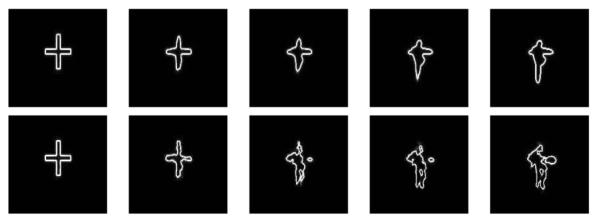
Warping results obtained for the “Soccer Player” training set, starting with an initial contour representing a “plus” sign. First row: Evolution obtained using kernel PCA. Second row: Evolution obtained using linear PCA. When kernel PCA is used, the final contour resembles the elements of the training set. In contrast, the final contour obtained using linear PCA bears little resemblance to the learned shapes.

Fig. 6b shows the warping results obtained by applying linear PCA on SDF. Fig. 6d shows the warping results obtained by applying linear PCA on binary maps. Note that the results obtained for the SDF representation bear little resemblance to the elements of the training sets. The results obtained for binary maps are more faithful to the learned shapes (see [36] for a more in-depth study of this fact). Figs. 6c and 6e presents the warping results obtained by applying kernel PCA on SDF and binary maps, respectively. In both cases, the final contour is very close to the training set and the results are better than any of the results obtained with linear PCA.

Fig. 6.

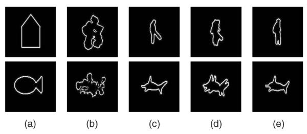
Warping results of an arbitrary shape, obtained using linear PCA and kernel PCA applied on both SDFs and binary maps. First row: Results for the “Soccer Player” training set. Second row: Results for the “Shark” training set. (a) Initial shape. (b) PCA on SDF. (c) Kernel PCA on SDF. (d) PCA on binary maps. (e) Kernel PCA on binary maps.

6.2.2 Robustness to Misalignment

In these experiments, the robustness of each method (linear and kernel PCA) to misalignments relative to the registered shapes of a training set is tested. This robustness to misalignment is an interesting property to evaluate since to perform segmentation, differences in pose (for example, translations) between the object of interest in the image and the registered training shapes need to be accounted for. Hence, whether a probabilistic method [1] or a gradient descent scheme [2] is used to compensate for these differences, more or less important misalignments between the contour and the registered training shapes may occur during the evolution process. This can impair the ability of the shape energy to properly constrain the shape of the segmenting contour.

In each of the following three experiments, an initial contour representing a chosen training shape for which pose differs from the registered training shapes is used as the initial contour for warping (SDFs were used to represent shapes). For the first initial contour, a small translation of about 5 pixels in the x and y-directions was performed. The second initial contour was a translation of about 10 pixels in the x and y-directions. Figs. 7 and 8 present the warping results obtained for the smaller and larger misaligned initial shapes, respectively. The first lines of Figs. 7 and 8 show the results obtained using KPCA; the second lines of Figs. 7 and 8 present the results using linear PCA. Once again, the results obtained with linear PCA bear little resemblance to the elements of the training sets. In contrast, the final contours obtained using kernel PCA are more faithful to the learned shapes. Besides, whether the initial contour is slightly or heavily misaligned, the contour evolution results in a translation of the contour when kernel PCA is used. Interestingly, the shape of the final contour obtained using KPCA is very much like the shape of the initial contour for both experiments. In Fig. 9, the initial contour represents one of the learned shapes scaled up by 10 percent and rotated by 10 degrees. As a result of warping using linear PCA, an unrealistic shape is obtained. In contrast, the final contour obtained when using kernel PCA is a realistic shape that is, in effect, rotated back and scaled down compared with the initial contour. Similar satisfying results were obtained with KPCA using binary maps as a representation of shapes. Hence, KPCA appears to offer a higher level of robustness than linear PCA to the misalignment of the initial contour (at least in the experiments we performed).

Fig. 7.

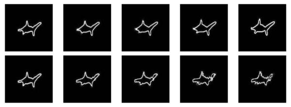
Warping results obtained for the “Shark” training set. The initial contour (leftmost image) represents one of the learned shapes slightly misaligned (5 pixels) with the corresponding element in the registered training set. First line: Evolution obtained using kernel PCA. Second line: Evolution obtained using linear PCA. The final contour obtained using kernel PCA resembles the elements of the training set and is positioned where the learned shapes were registered. The final contour obtained using linear PCA bears little resemblance to the learned shapes.

Fig. 8.

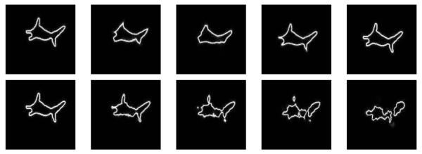
Warping results obtained for the “Shark” training set. The initial contour (leftmost image) represents one of the learned shapes misaligned by approximately 10 pixels. First line: Evolution obtained using kernel PCA. Second line: Evolution obtained using linear PCA.

Fig. 9.

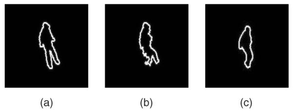
Warping results obtained for the “Soccer player” training set. (a) Initial contour representing one of the learned shapes scaled up by 10 percent and rotated by 10 degrees. (b) Final result using linear PCA (an unrealistic shape is obtained). (c) Final result using KPCA (the final contour is a realistic shape, effectively rotated and scaled down).

6.2.3 Multimodal Learning

Kernel methods have been used to learn complex multimodal distributions in an unsupervised fashion [9]. The goal of this section is to investigate the ability of kernel PCA to simultaneously learn objects of different shapes and to constrain the contour evolution in a meaningful fashion. Besides, we want to contrast the performances obtained with KPCA to the performances obtained with linear PCA. The “4 Words” training set was used for these experiments. Diverse contours, whose shapes bore some degree of resemblance to any of the four words (“orange,” “yellow,” “square,” or “circle”), were then used as initial contours for warping.

Each line in Fig. 10 presents the warping results obtained for the diverse initial contours used, for both linear and kernel PCA, using SDFs as representations of shape. The initial contour presented on the first line in Fig. 10a is the word “square” in which the letters are partially erased. The warping result using linear PCA bears little resemblance to the word “square.” In contrast, using kernel PCA, the word square is accurately reconstructed. In particular, a police close to the original one used in the initial contour is obtained. The initial contour presented on the second line in Fig. 10a is the word “circle” occluded by a line. Again, the warping result using linear PCA bears little resemblance to the word “circle” (a mixing of the different training words is obtained). Using KPCA, not only is the word “circle” accurately reconstructed, but the line is also completely removed. Besides, the original scheme used for the initial contour (which belongs to the training set) is preserved. The initial contour presented on the third line in Fig. 10a is the registered training word “yellow” slightly translated. The letter “y” is also replaced by a rectangle. Employing kernel PCA, the word “yellow” is perfectly reconstructed: The letter “y” is recovered, the contour is translated back, and the original police used for the initial contour is preserved. In comparison, the word “yellow” is barely recognizable from the final contour obtained using linear PCA.

Fig. 10.

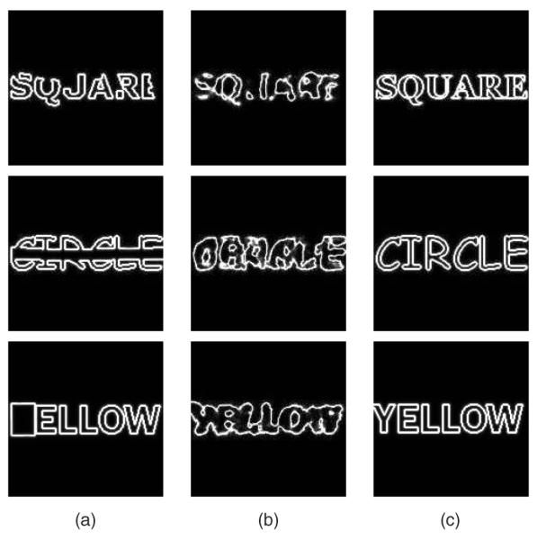
Warping results for the “4 Words” training set. (a) Initial contours. (b) Warping using linear PCA. (c) Warping using kernel PCA.

In each of the experiments above, the accurate word is detected and reconstructed using kernel PCA. Similar robust performances were obtained with kernel PCA on binary maps. The shape of the final contour obtained with linear PCA was oftentimes the result of a mixing between words of different classes. This mixing between classes can lead to unrealistic shapes. Thus, KPCA appears to be a strong method for introducing shape priors within the GAC framework when training sets involving different types of shapes are used.

6.2.4 Influence of the Parameter σ in Exponential Kernels

The goal of this section is to study the influence of the parameter σ when kernel PCA is performed using exponential kernels. Fig. 11 presents warping results of an arbitrary shape using different values of the parameter σ for the kernel defined in (8), which corresponds to performing kernel PCA on binary maps. The Shark training set was used for the shape learning.

Fig. 11.

Influence of σ for the kernel PCA method (exponential kernel) on binary maps. Warping results of an arbitrary shape are presented for the “Shark” training set. (a) Initial shape. (b) Warping result for σ = 3, (c) σ = 7, (d) σ = 9, (e) σ = 15.

As can be seen in Fig. 11, as the value of σ increases, more and more mixing among the shapes of the training set is allowed. Such shape mixing naturally occurs when linear PCA is used for learning (for example, in Fig. 6d, second row, this type of mixing can be observed). Similar results were obtained for the SDF representation and the kernel given in (7). Hence, the parameter σ allows for controlling the degree of “mixing” allowed among the learned shapes in the shape prior, which is another advantage of kernel PCA over linear PCA. The choice of σ should typically depend upon how much shape variation occurs within the data set. To emphasize this, larger σ’s allow for more mixing among the shapes, whereas smaller σs lead to more “selective” shape priors.

6.3 Segmentation Results: Image-Shape Model Only (No Shape Prior)

This section presents segmentation results of real and synthetic images obtained from using the image-shape segmentation technique presented in Section 4. No shape information was used to perform these segmentations. To ensure the smoothness of the contour, a classical curvature term which penalizes longer contours was introduced. Equation (1) was run until convergence using the expression of ∇_ϕE_image as given in (17).

Fig. 12 presents results obtained for each of the image-shape models (involving different intensity statistics) presented above. Fig. 12a represents a couple (darker intensities) on a lighter background. At each iteration of the contour evolution, an image-shape model was built, using the mean intensities inside and outside the curve. Fig. 12b is a synthetic image representing a square. The mean intensities inside and outside the square are the same; only the variances differ. Fig. 12c represents a zebra on a savannah plain. For both images, image-shape models were built from the probability distributions of the intensities inside and outside the curve at each evolution step. Satisfying segmentation results were obtained in each case, resulting in the accurate separation of the object of interest from the background.

Fig. 12.

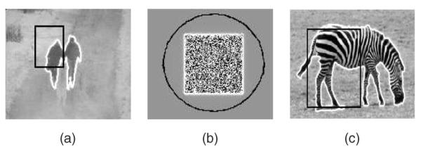
Segmentation results obtained using E_image from (16). The initial contour is in black and the final contour is in white. (a) Couple (dark) on lighter background, segmented using first moment only. (b) Two regions of same mean intensity and different variances segmented using global intensity distributions. (c) Zebra segmented using global intensity distributions.

6.4 Segmentation Results: Image-Shape Model + Shape Prior

This section presents segmentation results obtained by introducing shape prior using KPCA on binary maps and using our intensity-based segmentation methodology as presented in Section 5. For all of the following experiments, (1) was run until convergence on diverse images, using (22) as an energy functional (the parameter α was chosen to be α = 50%). In parallel, the transformation T[p] between the object of interest and the registered training set was recovered. No curvature term was used for contour regularization since smoothness information is indeed already present in the binary maps used to build shape priors.

6.4.1 Toy Example: Shape Priors Involving Objects of Different Types

The goal of this section is to investigate the ability of the algorithm described in Section 5 to accurately detect and segment objects of different shapes. For these experiments, the “4 Words” training set was used. We tested our algorithm on images where a corrupted version of the word “orange,” “yellow,” “square,” or “circle” was present (Fig. 13, first row). Word recognition is a challenging task and addressing it using GACs may not be a panacea. However, the ability of the level set representation to naturally handle topological changes was found to be useful for this purpose. During evolution, the contour split and merged a certain number of times to segment the disconnected letters of the words. In all of the following experiments, the same initial contour was used.

Fig. 13.

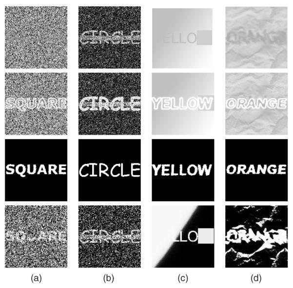
Segmentation results for the “4 Words” training set. Shape priors were built by applying the KPCA on binary maps. First row: Original images to segment. Second row: Segmentation results. Third row: Shape underlined by the final contour (Hϕ). Fourth row: Image-shape model (G_[I,ϕ(t)]) obtained when computing E_image for the final contour.

Experiment 1

In this experiment, the word “square” was corrupted: The letter “u” was almost completely erased. The shape thus obtained was filled with Gaussian noise of mean μ_o = 0.5 and variance σ_o = 0.05. The background was also filled with Gaussian noise of the same mean μ_b = 0.5 but of variance σ_b = 0.2. The result of applying our method is presented Fig. 13a. The image-shape model was built using the method involving global statistics described in Section 4.2. Despite the noise and the partial deletion, a convincing segmentation and a smooth contour are obtained. In particular, the correct font is detected and the letter “u” is accurately reconstructed.

Experiment 2

In this second experiment, one of the elements of the training set was used. A thick line (occlusion) was drawn on the word and a fair amount of Gaussian noise was added to the resulting image. The result of applying our method is presented in Fig. 13b. Despite the noise and the occlusion a very convincing segmentation is obtained. In particular, the correct font is detected and the thick line is completely removed. Once again, the final contour is smooth despite the fairly large amount of noise.

Experiment 3

In this third test, the word “yellow” was written using a different font from the ones used to build the training set. In addition, “linear shadowing” was used in the background, making the first letter “y” completely hidden. The letter “w” was also replaced by a gray square. The result of applying our framework is presented in Fig. 13c. The word “yellow” is correctly recognized and segmented. In particular, the letters “y” and “w” were completely reconstructed.

Experiment 4

In this experiment, the word “orange” was handwritten in capital letters roughly matching the size of the letters of the words in the training set. The intensity of the letters was chosen to be rather close to some parts of the background. In addition, the word was blurred and smeared in a way that made its letters barely recognizable. This type of blurring effect is often observed in medical images due to patient motion. This image is particularly difficult to segment, even when using shape prior, since the spacing between letters and the letters themselves are very irregular due to the combined effects of handwriting and blurring. Hence, mixing among classes (confusion between any of the four words) can be expected in the final result. In the final result obtained, the word “orange” is not only recognized but satisfyingly recovered; in particular, a thick font was obtained to model the thick letters of the word (Fig. 13d).

Hence, starting from the same initial contour in each experiment, our algorithm was able to accurately detect which word was present in the image. This highlights the ability of our method not only to gather image information throughout evolution but also to distinguish between objects of different classes (“orange,” “yellow,” “square,” and “circle”). Comparing the final contours obtained in each experiment to the final image-shape model G_[I,ϕ(t)] (last row in Fig. 13), one can measure the effect of our shape prior model in constraining the contour evolution. The image information alone would lead to a shape bearing very little resemblance to any of the learned words.

6.5 Real-Image Examples: Tracking Temporal Sequences

To test the robustness of the framework, tracking was performed on two sequences. A very simple tracking scheme was used with the same initial contour being used for each image in the sequence. This contour was initially positioned wherever the final contour was in the preceding image. Of course, many efficient tracking algorithms have already been proposed. However, convincing results were obtained here, without considering the system dynamics, for instance. This highlights the efficiency of including prior knowledge on shape for the robust tracking of deformable objects. The parameter α was fixed to α = 55 percent in (22) to make up for the influence of clutter in the images. The nice tracking performance observed, despite the fact that parameters are fixed throughout the sequence, further highlights the robustness of the proposed segmentation framework.

6.5.1 Soccer Player Sequence

In this sequence (composed of 130 images), a man is playing with a soccer ball. The challenge is to accurately capture the large deformations due to the movement of the person (for example, limbs undergo large changes in aspect) while sufficiently constraining the contour to discard clutter in the background. The training set of 22 silhouettes, presented in the first row of Fig. 14, was used. The version of E_image involving the intensity means only was used to capture image information. Despite the small number of shapes used for training and the initialization of the contour evolution with the same (arbitrary) contour, successful tracking was obtained, correctly capturing the very diverse postures of the player.

Fig. 14.

Tracking results with the proposed method. First row: Soccer Player sequence (the rightmost frame is the result obtained without shape prior; α = 1 in (22)). Second row: “Shark” sequence (the rightmost frame is an original image from the sequence, reproduced here to assess the poor level of contrast).

6.5.2 Shark Video

In this sequence (composed of 70 images), a shark is evolving in a highly cluttered environment. Note that the shark is at times partially occluded by other fish and has poorly contrast. To perform tracking, 15 shapes were extracted from the first half of the video (second row of Fig. 14) and used to build the shape prior. The version of E_image involving global statistics was used to make up for the poor contrast of the shark in the images. Once again, despite the small training set, successful tracking performances were observed. The shark was correctly captured, while clutter and occlusions were rejected.

7 Conclusions

In this paper, we used an unsupervised learning technique to introduce shape priors in the GAC framework. Our approach uses KPCA, a technique borrowed from the machine learning community. We employed the projections on the learned spaces of shapes (using either linear PCA or kernel PCA) as models. The projections on the learned spaces appear to be more representative than the commonly used average of the (mapped) data when dealing with multimodal distributions. Further, using such models allows for comparing learning techniques in a rigorous manner. For each learning technique, the same initial contour can be deformed (using the projection on the corresponding learned space as a model) and the final contours thus obtained can be compared in terms of their similarity with the elements of the training sets. This approach allows for investigating the performance of each learning method without using any image information. Using this technique, better performance of kernel PCA as compared to linear PCA was demonstrated for two representations of shapes (binary maps and SDFs).

In addition, we proposed a region-based approach aimed at separating an object from the background. This method consists of extracting an image-shape model from the image to direct the evolution of the contour. The technique can successfully deal with diverse image intensity statistics. In the present work, we also highlighted the importance of expressing image and shape energies in a consistent manner. This is especially important when dealing with nonlinear techniques such as KPCA. Valuable insights about the pitfalls of balancing forces extracted directly from the feature space with “linear” (image) forces were obtained from the study of one-dimensional approximations. A method for addressing some of the potential problems was also proposed which drastically improved balancing performances. In the proposed algorithm, image information and shape knowledge are combined in a consistent fashion, both energies are expressed in terms of shapes, and meaningful balances between image information and shape knowledge are realized.

Finally, very reasonable segmentation performances were obtained on complex images, highlighting the power and accuracy of the proposed framework. The method not only allowed us to simultaneously learn shapes of different objects but was also robust to noise, blurring, occlusion, and clutter.

In this paper, the image-shape model G_[I,ϕ] was considered to be constant between two evolution steps. Interesting additional segmentation properties can be observed by also considering the variation of G_[I,ϕ] in the computation of ∇_ϕE_image; these properties will be studied in detail in our future work. In addition, we plan to investigate the performance of other kernels to introduce shape priors within the GAC framework. Our goal is to apply the proposed framework on 3D medical images. The precision and robustness afforded by the proposed technique will hopefully be a valuable asset for automated medical segmentation.

Biography

Samuel Dambreville received the master of science degree in electrical engineering and the master’s degree in business administration from the Georgia Institute of Technology in 2003 and 2006, respectively, and the “Diplome d’ingenieur en Genie Electrique et Automatique” (MEng) from the ENSEEIHT, Toulouse, France, in 2003. He is currently a PhD candidate in the School of Electrical and Computer Engineering at the Georgia Institute of Technology. His research interests include the robust tracking of deformable objects and the development of statistical and shape-driven techniques for active contour segmentation. He was the recipient of the Hugo O. Schuck Best Paper Award at the 2007 American Control Conference (along with Yogesh Rathi and Allen Tannenbaum). He is a student member of the IEEE.

Yogesh Rathi received the bachelor’s degree in electrical engineering and the master’s degree in mathematics from the Birla Institute of Technology and Science, Pilani, India, in 1997 and the PhD degree in electrical engineering from the Georgia Institute of Technology, Atlanta, in 2006. His PhD thesis entitled “Filtering for Closed Curves” was on tracking highly deformable objects in the presence of noise and clutter. He is currently a postdoctoral fellow in the Psychiatry Neuroimaging Laboratory at Brigham and Women’s Hospital, Harvard Medical School, Boston. His research interests include image processing, medical imaging, diffusion tensor imaging, computer vision, control, and machine learning. He is a member of the IEEE.

Allen Tannenbaum is a faculty member in the Schools of Electrical and Computer and Biomedical Engineering at the Georgia Institute of Technology. His research interests include systems and control, computer vision, and image processing. He is a member of the IEEE.

REFERENCES

- [1].Leventon M, Grimson E, Faugeras O. Statistical Shape Influence in Geodesic Active Contours. Proc. IEEE Conf. Computer Vision and Pattern Recognition.2000. pp. 1316–1324. [Google Scholar]
- [2].Tsai A, Yezzi T, Wells W. A Shape-Based Approach to the Segmentation of Medical Imagery Using Level Sets. IEEE Trans. Medical Imaging. 2003;vol. 22(no 2):137–153. doi: 10.1109/TMI.2002.808355. [DOI] [PubMed] [Google Scholar]
- [3].Yezzi A, Kichenassamy S, Kumar A. A Geometric Snake Model for Segmentation of Medical Imagery. IEEE Trans. Medical Imaging. 1997;vol. 16:199–209. doi: 10.1109/42.563665. [DOI] [PubMed] [Google Scholar]
- [4].Yezzi A, Soatto S. Deformotion: Deforming Motion, Shape Average and the Joint Registration and Approximation of Structures in Images. Int’l J. Computer Vision. 2003;vol. 53:153–167. [Google Scholar]
- [5].Cootes T, Taylor C, Cooper D. Active Shape Models—Their Training and Application. Computer Vision and Image Understanding. 1995;vol. 61:38–59. [Google Scholar]
- [6].Wang Y, Staib L. Boundary Finding with Correspondence Using Statistical Shape Models. Proc. IEEE Conf. Computer Vision and Pattern Recognition.1998. pp. 338–345. [Google Scholar]
- [7].Cremers D, Kohlberger T, Schnoerr C. Diffusion Snakes: Introducing Statistical Shape Knowledge into the Mumford-Shah Functional. Int’l J. Computer Vision. 2002 Feb.vol. 50:295–313. [Google Scholar]
- [8].Cremers D, Kohlberger T, Schnoerr C. Shape Statistics in Kernel Space for Variational Image Segmentation. Pattern Recognition. 2003;vol. 36:1292–1943. [Google Scholar]
- [9].Mika S, Schölkopf B, Smola AJ, Müller K-R, Scholz M, Rätsch G. Advances in Neural Information Processing Systems. vol. 11. MIT Press; 1999. Kernel PCA and De-Noising in Feature Spaces. [Google Scholar]
- [10].Sapiro G, editor. Geometric Partial Differential Equations and Image Analysis. Cambridge Univ. Press; 2001. [Google Scholar]
- [11].Osher SJ, Sethian JA. Fronts Propagation with Curvature Dependent Speed: Algorithms Based on Hamilton-Jacobi Formulations. J. Computational Physics. 1988;vol. 79:12–49. [Google Scholar]
- [12].Rousson M, Paragios N. Shape Priors for Level Set Representations. Proc. Seventh European Conf. Computer Vision.2002. pp. 78–92. [Google Scholar]
- [13].Cremers D, Osher S, Soatto S. Kernel Density Estimation and Intrinsic Alignment for Knowledge-Driven Segmentation: Teaching Level Sets to Walk. Proc. 26th DAGM Pattern Recognition Symp..2004. pp. 36–44. [Google Scholar]
- [14].Dambreville S, Rathi Y, Tannenbaum A. Shape-Based Approach to Robust Image Segmentation Using Kernel PCA. Proc. IEEE Conf. Computer Vision and Pattern Recognition; 2006. pp. 977–984. [PMC free article] [PubMed] [Google Scholar]
- [15].Sethian JA. Level Set Methods and Fast Marching Methods. Cambridge Univ. Press; 1999. [Google Scholar]
- [16].Osher S, Fedkiw R. Level Set Methods and Dynamic Implicit Surfaces. Springer; 2003. [Google Scholar]
- [17].Paragios N, Chen Y, Faugeras O. Handbook of Mathematical Models in Computer Vision. Springer; 2005. [Google Scholar]
- [18].Schölkopf B, Mika S, Müller K. Nonlinear Component Analysis as a Kernel Eigenvalue Problem. Neural Computation. 1998;vol. 10:1299–1319. [Google Scholar]
- [19].Kwok J, Tsang I. The Pre-Image Problem in Kernel Methods. IEEE Trans. Neural Networks. vol. 15:1517–1525. doi: 10.1109/TNN.2004.837781. [DOI] [PubMed] [Google Scholar]
- [20].Rathi Y, Dambreville S, Tannenbaum A. Comparative Analysis of Kernel Methods for Statistical Shape Learning. Proc. Second Int’l Workshop Computer Vision Approaches to Medical Image Analysis.2006. pp. 96–107. [Google Scholar]
- [21].Mercer J. Functions of Positive and Negative Type and Their Connection with the Theory of Integral Equations. Philosophical Trans. Royal Soc. of London. 1909;vol. 209:415–446. [Google Scholar]
- [22].Schölkopf B, Mika S, Müller K. An Introduction to Kernel-Based Learning Algorithms. IEEE Trans. Neural Networks. 2001;vol. 12:181–201. doi: 10.1109/72.914517. [DOI] [PubMed] [Google Scholar]
- [23].Yezzi A, Tsai A, Willsky A. A Statistical Approach to Snakes for Bimodal and Trimodal Imagery. Proc. Int’l Conf. Computer Vision.1999. pp. 898–903. [Google Scholar]
- [24].Chan T, Vese L. Active Contours without Edges. IEEE Trans. Image Processing. 2001;vol. 10(no 2):266–277. doi: 10.1109/83.902291. [DOI] [PubMed] [Google Scholar]
- [25].Rousson M, Deriche R. A Variational Framework for Active and Adaptative Segmentation of Vector Valued Images. Proc. IEEE Workshop Motion and Video Computing.2002. p. 56. [Google Scholar]
- [26].Paragios N, Deriche R. Geodesic Active Regions for Supervised Texture Segmentation. Proc. Int’l Conf. Computer Vision.1999. pp. 926–932. [Google Scholar]
- [27].Paragios N, Deriche R. Geodesic Active Regions: A New Paradigm to Deal with Frame Partition Problems in Computer Vision. J. Visual Comm. and Image Representation. 2002;vol. 13:249–268. [Google Scholar]
- [28].Caselles V, Kimmel R, Sapiro G. Geodesic Active Contours. Int’l J. Computer Vision. 1997;vol. 22:61–79. [Google Scholar]
- [29].Kichenassamy S, Kumar S, Olver P, Tannenbaum A, Yezzi A. Conformal Curvature Flow: From Phase Transitions to Active Vision. Archives for Rational Mechanics and Analysis. 1996;vol. 134:275–301. [Google Scholar]
- [30].Zhu SC, Yuille AL. Region Competition: Unifying Snakes, Region Growing, and Bayes/MDL for Multiband Image Segmentation. IEEE Trans. Pattern Analysis and Machine Intelligence. 1996 Sept.vol. 18(no 9):884–900. [Google Scholar]
- [31].Morel J-M, Solimini S. Variational Methods for Image Segmentation. Birkhauser; 1994. [Google Scholar]
- [32].Kim J, Fisher J, Yezzi A, Cetin M, Willsky A. Nonparametric Methods for Image Segmentation Using Information Theory and Curve Evolution. Proc. Int’l Conf. Image Processing; 2002. pp. 797–800. [DOI] [PubMed] [Google Scholar]
- [33].Rathi Y, Michailovich O. Seeing the Unseen: Segmenting with Distributions. Proc. Int’l Conf. Signal and Image Processing.2006. [Google Scholar]
- [34].Duda R, Hart P, Stork D. Pattern Classification. Wiley-Interscience; 2001. [Google Scholar]
- [35].Rathi Y, Dambreville S, Tannenbaum A. Statistical Shape Analysis Using Kernel PCA. Proc. SPIE. 2006;vol. 6064:425–432. [Google Scholar]
- [36].Dambreville S, Rathi Y, Tannenbaum A. A Shape-Based Approach to Robust Image Segmentation. Proc. Int’l Conf. Image Analysis and Recognition; 2006. pp. 173–183. [PMC free article] [PubMed] [Google Scholar]