

1. Introduction
Samples studied with conventional magnetic resonance (MR) techniques are subjected to a polarizing static magnetic field . Ideally, this magnetic field is assumed to be spatially homogeneous over the sample volume. However, the presence of any object of finite magnetic susceptibility (i.e. a sample) will inevitably perturb this magnetic field and provide the Larmor frequencies of MR-sensitive spins with an unwanted spatial dependence. These susceptibility-induced B0 perturbations, which are a fundamental result of Maxwell’s electromagnetic field theory, scale roughly linearly in magnitude with applied B0 field strengths.
B0 inhomogeneity degrades the signal-to-noise ratio (SNR) of all MR measurements. While Hahn spin-echoes can be used to refocus B0 inhomogeneity at one instantaneous temporal point, the remainder of a spin-echo is tempered by B0 inhomogeneity-induced signal relaxation (commonly referred to as ). Furthermore, many techniques cannot utilize spin-echo procedures, and are thus susceptible to the full evolution of relaxation.
The spatial variation of Larmor frequencies within a spectro-scopic voxel will broaden and distort spectral lineshapes. Standard spectroscopic techniques such as frequency-selective resonance suppression and spectral editing are easily degraded by these effects.
MR images are susceptible to the same B0-induced SNR deterioration as spectroscopic acquisitions. Additionally, they can further suffer from spatial distortion in regions of high B0 inhomogeneity. In particular, commonly utilized rapid imaging strategies such as steady-state free precession (SSFP), spiral, and echo-planar imaging (EPI) are often compromised by B0 inhomogeneity.
Broadly speaking, B0 shimming refers to the optimized application of external magnetic fields to compensate unwanted inhomogeneity of the B0 magnetic field. For applications that require high-degrees of B0 homogeneity, fine-tuned shimming has historically been accomplished using sets of dedicated electromagnets. These electromagnet coils, or ‘active shims’, can be adjusted on a subject-specific basis.
This review is focused on high-field B0 shimming of the brain, specifically within small rodents and humans. B0 field perturbations within the brain are particularly prominent near the air-tissue interfaces at the sinus and auditory cavities. The recent increases of B0 field strengths used in both clinical and research MR systems necessitates maximal utility of conventional shim technology. For some applications, this conventional technology cannot adequately homogenize designated shim volumes (particularly larger volumes). Therefore, along with the development of automated optimization protocols for conventional active shim systems, recent investigations have explored alternative approaches to shim hardware design.
A theoretical treatment of B0 inhomogeneity and its effects on magnetic resonance acquisitions are presented in the next section. Section 3 then presents the techniques utilized in MR-based mapping of static magnetic fields, which is now a standard tool in automated shimming methods. The hardware and methods utilized in room-temperature shimming (also commonly referred to as ‘active’ shimming) are developed in Section 4. The challenges of optimizing B0 homogeneity over extended volumes are introduced in Section 5, followed by a discussion of the methods and capabilities of Dynamic Shim Updating (DSU) of room-temperature shims. Finally, recent novel approaches to shimming that deviate from any previous technological methodologies, such as local active shimming and subject-specific passive shimming, are presented.
2. Theory
An in vivo MR system will typically have RMS B0 homogeneity of up to only about 50 parts-per-million (ppm) of the static magnetic field strength (≈6 kHz at 3T) over manufacturer-defined diameter spherical volumes (DSVs). Typical DSV diameters are roughly 45 cm for human systems and 5–6 cm for small animal systems. This inherent magnetic field inhomogeneity arises from a number of factors. First, it is extremely difficult to generate homogeneous current density distributions in superconducting magnet systems. The resulting winding errors distort the idealized homogeneous magnetic field produced by an infinite solenoid. Intense electromagnetic and gravitational forces can also alter the magnet geometry as the system settles over time. Such settling is not predictable and tends to thwart even the most ingenious magnet designs.
When a magnet is commissioned, it undergoes a shimming procedure to minimize the subject-independent background B0 inhomogeneity. This is accomplished primarily by two methods. In a passive-shimming technique known as ferroshimming, iron or steel pieces can be strategically placed around the bore of the magnet [1]. A number of optimization schemes have been developed to accomplish this task [2]. Most magnets are also equipped with sets of superconducting electromagnetic shims that can be optimized upon magnet commissioning to compensate background inhomogeneity. Using these approaches, subject-independent background B0 inhomogeneity is typically reduced to less than 1.5 ppm (≈240 Hz at 3T) over prescribed DSVs.
Of far greater concern to in vivo magnetic resonance experiments is the B0 inhomogeneity induced by the placement of samples in an MR apparatus. The magnitude and distribution of subject-specific B0 inhomogeneity depends heavily upon the applied B0 magnetic field and the magnetic susceptibility distributions of specific samples. Such perturbations to the static magnetic field are particularly troublesome in vivo, where magnetic susceptibility boundaries between anatomic air cavities (χ ≈ 0.3 ppm) and biological tissue (χ≈−9.2 ppm) generate significant field gradients. Furthermore, macroscopic susceptibility distributions can vary widely across species (e.g. from rat to mouse), within species (e.g. the brains of different human subjects), and dynamically in time (e.g. due to respiration). Means to actively reduce B0 inhomogeneity are therefore of crucial concern for many high-field in vivo MR applications.
2.1. Magnetostatics of sample-induced B0 inhomogeneity
Given a distribution of magnetizable material M(r), the magnetic induction B(r) is related to the auxiliary field H(r) according to
| (1) |
where μ0 is the permeability of free space.
Diamagnetic and paramagnetic substances have a linear relation between B and H,
| (2) |
where μ is the magnetic permeability. This relation is nonlinear for ferromagnetic materials.
For materials of small magnetic susceptibility, it is convenient to express the magnetic permeability in terms of μ0,
| (3) |
where χ is the magnetic susceptibility. Using Eqs. (1)-(3), the magnetization can be expressed as
| (4) |
In the absence of free-currents, the magnetic scalar potential can be utilized,
| (5) |
The scalar potential abides by the Poisson relation
| (6) |
In reality, magnetization distributions have spatial discontinuities. Given a boundary between two regions of magnetizations M1 and M2 spanning a surface 𝒮, a discontinuity condition
| (7) |
is established. Along the boundary surface 𝒮, an effective magnetic ‘surface charge’ of density σM = n · ≈ Δ M is induced, where n is a unit vector normal to 𝒮.
With these definitions, the general solution to Eq. (6) is then given by
| (8) |
For samples typically encountered in magnetic resonance experiments, homogeneous magnetization compartments can usually be assumed. This then nulls the volume integration and leaves
| (9) |
To demonstrate how this equation can be used to predict B0 inhomogeneity, consider the perturbation induced by a sphere of radius a and constant susceptibility χ surrounded by free space in a uniform magnetic field, . Using the assumption that |χ| < < 1 (which is valid for materials considered in this review) with Eqs. (2) and (4), the approximation
| (10) |
can be applied. On the surface of the sphere, this magnetization induces a magnetic surface charge given by
| (11) |
The Greens function in Eq. (9) can be expanded in spherical harmonics, Ylm(θ, ϕ) [3], as
| (12) |
where (r, θ, ϕ) are spherical polar coordinates and r< = min(r’, r) and r> = max(r’, r).
For problems of azimuthal symmetry, we can set m = 0:
| (13) |
where Pl are the Legendre polynomials. Given these considerations, Eq. (9) yields
| (14) |
Using the orthogonality relation
| (15) |
we then have
| (16) |
Simplification of the radial coordinate condition and Cartesian substitution then gives
| (17) |
where . Again applying the small-susceptibility-approximation to Eqs. (2) and (5), the component of the magnetic induction is then given by
| (18) |
and the magnetic field induced by the sphere is
| (19) |
Note that the induced field external to the sphere is equivalent to that of a dipole with magnitude
| (20) |
The first-order approximation utilized in this analytic derivation also enables rapid numerical estimation of Eq. (8) for arbitrary magnetic susceptibility distributions placed in an MR apparatus [4-6]. Section 3.3 will discuss these methods and applications in more detail.
2.1.1. Categories of B0 field perturbations
We have now established that placement of a magnetically susceptible material in a B0 field can spatially distort a perfectly homogeneous B0 source field. In vivo B0 distortions can be divided into microscopic, mesoscopic, and macroscopic contributions. Microscopic B0 effects have spatial variations on the order of molecular and atomic sizes. Mesoscopic contributions have variations that are much smaller than a typical imaging voxel, yet far greater than molecular and atomic sizes. Macroscopic contributions vary over dimensions greater than an imaging voxel [7]. Field variations on a microscopic level contribute to spin relaxation processes, while those on a mesoscopic level contribute to phenomena such as those monitored with the BOLD effect [8-10]. Macroscopic susceptibility inductions result from large-scale susceptibility variations within a sample and it is those which are targeted for compensation with shim hardware.
2.2. The impact of B0 inhomogeneity
B0 inhomogeneity can have a variety of effects on MR images. Its impact on image-quality depends heavily on the variety and timing of a given MRI acquisition.
Cartesian k-space sampling shows the most readily visible effects of B0 inhomogeneity. In a Cartesian acquisition, the primary effects of B0 inhomogeneity are signal loss and image distortion. Receiver bandwidths (and correlated gradient strengths) significantly impact the degree of image distortion caused by spatial variation of B0 field offsets. In the face of only anatomically driven inhomogeneity (i.e. not caused by the presence of implants or external devices), typical imaging bandwidths for standard spin-echo and gradient-echo imaging sequences result in limited image distortion.
Banding artifacts can be found in regions of high inhomogeneity when imaging with steady-state free precession (SSFP) techniques (FIESTA, TrueFISP) [11]. In the presence of unwanted field gradients, the steady-state condition in an SSFP sequence will periodically degrade across the image volume. This degradation of the steady state results in phase cancellation across the image and manifests itself as bands of signal dropout emanating from regions of high inhomogeneity.
It is possible to greatly reduce banding artifacts in SSFP imaging by making additional image acquisitions with differing steady state phases (for example, with RF phase-cycling) and combining the final images through either a maximum intensity projection (MIP), a sum of squares (SOS), a complex sum, or a magnitude sum. It has been reported that the SOS combination has optimal performance [12].
For non-Cartesian k-space trajectories (spiral, projection reconstruction), B0 inhomogeneity distorts and/or provides unwanted weighting to intended k-space trajectories [13]. This results in blurred and distorted reconstructed images and can have a significant impact on image quality.
2.2.1. Echo-planar image distortion
The quality and reliability of single-shot echo-planar-imaging (EPI) sequences are highly dependent on anatomically driven B0 inhomogeneity. This is largely due to the significantly reduced spatial encoding bandwidth used in the phase-encoded dimension of echo-planar images.
The generalized on-resonance imaging signal including B0 inhomogeneity for an infinitely thin two-dimensional slice is given by
| (21) |
where ρ is the spin density, Λ is a global detection constant (assuming spatial B1 homogeneity), x is the readout direction, and y is the phase-encoded direction. For an EPI experiment, the time (t) can be divided into increments
| (22) |
where n is the kx encoding step (sampling position), m is the ky phase encoding step (readout line), N is the total number of sampled points (in the readout), M is the total number of phase-encoded readouts per shot in the EPI experiment, and BW is the receiver bandwidth [14]. This definition modifies the signal according to
| (23) |
It is then convenient to define read and phase k-space encoding variables for an EPI experiment,
| (24a) |
| (24b) |
where Gx is the readout gradient strength, Gy is the strength of the blipped phase encode gradient, and TP is the blip duration. Using these definitions, n and m can be removed from Eq. (23),
| (25) |
The echo time (TE) results in a time delay from excitation to the middle of the echo readout train and will impact ΔB0-induced signal loss. Spin echo EPI experiments can be executed which rephase the signal at t = 0 (the echo-time), thus eliminating this term. However, any EPI strategy will have positional shifts given by
| (26a) |
| (26b) |
which are clear when applying the Fourier transform shift theorem to Eq. (25). These expressions can be expressed in a gradient-independent form using
| (27a) |
| (27b) |
Removing Gx, Gy, TP, and expressing the positional shifts in pixels gives,
| (28a) |
| (28b) |
This is a slightly simplified analysis whereby infinitesimal gradient rise times have been assumed. However, it is easily seen in this analysis that the shifts in the read and phase-encode directions are related by
| (29) |
The phase-encode direction will therefore have distortion exacerbated by a factor of M (number of phase-encode steps per shot) compared to that of the readout direction. For example, with a single-shot EPI acquisition grid of 64 × 64 pixels and a bandwidth of 200 kHz, a position with a B0 offset of 200 Hz will have an encoded readout shift of 0.06 pixels and a phase-encoded shift of 4 pixels. Therefore, it is clear that the phase-encode direction is the most significant consideration in EPI geometric distortion. Within both the human and rodent brains at B0 field strengths ≥3T it is not uncommon to encounter B0 offsets over 200 Hz. The resulting phase-encode pixel shifts are a significant problem in EPI-based applications. Notice that the phase-encoded distortion decreases when the number of phase-encoded steps per shot is decreased. At the expense of acquisition time (a strong constraint for many EPI applications), multiple-shot EPI can therefore be used to reduce the effects of EPI image distortion.
Diffusion tensor imaging (DTI) relies on contrast developed by the dephasing of diffusing spins moving through applied gradients. This contrast can be impacted by the presence of B0 field perturbations, therefore compromising quantitative DTI measurements [15]. However, even more problematic is the reliance of DTI methods on single-shot EPI techniques. DTI protocols often use rapid single-shot EPI to minimize patient motion during the collection of various independent images used to construct diffusion-tensor components. The B0 inhomogeneity-induced distortion in these images greatly displaces the white-matter fibers measured with DTI from their true location as depicted in the anatomic MRI.
2.2.2. Signal reduction
In seeming contradiction to the relaxation theory of Bloembergen, Purcell, and Pound (BPP) [16], empirically measured T2 values decrease significantly with increasing B0 field strengths [17]. This effect is sufficiently explained by Michaeli et al. [18] as the result of increased dynamic dephasing due to stronger microscopic magnetic susceptibility gradients at high magnetic field strengths. Spins diffusing through these mesoscopic field gradients lose phase coherence, which results in a shorter T2 measurement. Since diffusion is a random process, this effect cannot be refocused using Hahn spin-echoes, but can only be reduced by decreasing the time spins are allowed to diffuse. The effect can be partially removed using CPMG spin-echoes. Comparison of Hahn and CPMG spin-echo measurements can be used to quantify diffusion processes. Erwin Hahn’s seminal paper on spin-echo generation [19] predicted this effect, where the contribution of diffusion through field gradients resulted in what was then introduced as the modified transverse decay effect. Over time, the non-random dispersion of static spins in the presence of field gradients has also become known as decay. Therefore, decay must now classified as accruing in either the static (coherent) or dynamic (i.e. random diffusion-influenced) dephasing regimes [20].
For a gradient echo acquisition, signal loss in the static dephasing regime is a significant consideration. Consider a Cartesian-sampled gradient-echo sequence. Using the conventions defined above, spins at readout position i =1 ߪ N will undergo B0 inhomogeneity dephasing for a time , where TS = N/BW is the total sampling time. For an imaging sequence where TE is much greater than sampling time (TE ⪢ TS), it can be assumed that all signal samples are experiencing the same attenuation from B0-induced phase dispersion. However, when the above inequality is not satisfied, signal-loss induced k-space weighting must be considered.
Neglecting RF limitations (homogeneity and/or excitation/refocusing bands), signal loss is not dependent upon the absolute frequency offset, but rather upon the spatial field variation within voxels. Typical imaging voxels are small enough that a first-order Taylor expansion can be used to approximate the generalized spatial B0 variation about the center of the voxel. Using the aforementioned assumption that TE ⪢ N/BW, all pixels in the image will have B0-induced signal loss determined primarily by the local gradients across each pixel. Under this approximation, consider the free-induction signal (neglecting T2 effects) in a single cubic pixel of length L with homogeneous spin density ρ0 located at r =(x0, y0, z0). It can be shown that the magnitude [21] of this measured signal can be approximated as
| (30) |
The signal magnitude for pixels in the absence of B0 inhomogeneity would be given by
| (31) |
Therefore, the ratio of remaining signal in the presence of B0 inhomogeneity is given by
| (32) |
Because it is unrecoverable, signal loss in EPI is typically a far greater problem than image distortion. This is particularly the case in -weighted acquisitions. Within the brain, EPI is heavily utilized in measurement of the BOLD effect in fMRI and diffusion properties in diffusion tensor imaging (DTI). Since BOLD observation requires weighting, TE is typically extended to 35–50 ms in order to develop acceptable contrast. At such echo-times, signal loss from macroscopic B0 inhomogeneity (i.e. not the mesoscopic effects measured by the BOLD signal) can become particularly problematic.
Fig. 1 shows (A) a fast-spin-echo (FSE) anatomic image of an axial slice (6 mm thick) through the frontal cortex of the human brain at B0 = 3T, (B) a ΔB0 field map over the same slice, (C) signal loss in weighted (TE = 35 ms) gradient-echo images (most prominent loss indicated with orange arrow), and (D) distortion in EPI images (indicated with green arrows), collected with TE = 25 ms, 64 × 64 in plane pixels over a 20 cm × 20 cm FOV, a readout bandwidth of 250 kHz. Arrows indicate directions of distortion in the phase-encoded dimension. The effects of B0 inhomogeneity on signal loss and EPI geometric distortion are clear.
Fig. 1.
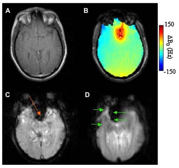
(A) Fast-spin-echo (FSE) anatomic image of an axial slice (6 mm thick) through the frontal cortex of the human brain at B0 = 3T. (B) ΔB0 field map over the same slice, (C) signal loss in weighted (TE = 35 ms) gradient-echo images (most prominent loss indicated with orange arrow), and (D) distortion in EPI images (indicated with green arrows), collected with TE = 25 ms, 64 × 64 in plane pixels over a 20 cm ×20 cm FOV, a readout bandwidth of 250 kHz. Arrows indicate directions of distortion in the phase-encoded dimension.
2.2.3. Spectroscopy
Magnetic resonance spectroscopy (MRS) has evolved into a widely utilized tool in both the research and clinical MR communities. Within the brain, MRS can enable non-invasive assessment of neurochemical concentrations on both a spatial and temporal basis. Due to the complexity of spectroscopic analysis and quantification, most MRS applications require careful consideration of B0 homogeneity over acquired spectroscopic volumes [22].
The linewidths and signal-to-noise ratio (SNR) of magnetic resonance spectra are ultimately determined by . Furthermore, while is often expressed as a monoexponential decay, the effects of B0 inhomogeneity on effective transverse relaxation are more complicated (as briefly discussed in Section 2.2.2). Across a spectroscopic voxel, will commonly have a polyexponential character, which then not only broadens spectra and decreases SNR, but also can cause lineshapes to deviate from a Lorentzian distribution. This in turn can lead to spectral quantification errors when the spectral shapes differ from utilized models.
Many spectroscopic techniques also require selective RF perturbation of specific resonances. Standard practices such as frequency-selective water suppression [23] and spectral editing rely on such capabilities. B0 inhomogeneity compromises these methods by both broadening the spectral widths needed for selective operations and displacing resonance frequencies on a spatial basis. Fig. 2 shows sample water-suppressed metabolite spectra acquired in two regions of the brain possessing different levels of local field homogeneity.
Fig. 2.

Water-suppressed proton spectra of two voxels, indicated in an axial MRI (B), where local field inhomogeneity (B0 =4T) is dramatically greater in one (anterior) of the voxels. Compared to the spectrum in the posterior voxel (C), spectral linewidths and water suppression are clearly degraded in the anterior voxel (D) due to the degraded field homogeneity in its locality. The presented field map (A) displays the field inhomogeneity causing increased linewidths and reduced water suppression in the anterior voxel.
MRS benefits from increased B0 field strengths due to increased SNR [24] and improved spectral dispersion. However, both of these gains are tempered by increases in B0 inhomogeneity, which also increases with B0 field strength. B0 shimming is therefore of crucial importance in utilizing higher B0 field strengths to improve spectroscopic capabilities.
In the previous sections, the origins of B0 inhomogeneity and its impact on MR capabilities have been highlighted and discussed. The next section will discuss means by which B0 inhomogeneity can be measured and assessed.
3. Magnetic field mapping
3.1. Principles
The basic principle of MRI-based B0 field mapping relies upon quadrature (complex) detection of the MR signal. Quadrature detection provides information on the angular phase (ϕ) of measured transverse magnetization. The phase of the measured magnetization advances with echo-time TE, according to
| (33) |
where ϕ0 is the initial phase of the magnetization imparted by RF excitation and ω is related to the local magnetic field offset by,
| (34) |
Here, B0 is the applied static magnetic field, ωCS is the chemical shift, and ΔB0 is a local magnetic field offset. If chemical shifts are neglected (i.e. assuming no lipid contamination in the mapped spin ensemble) and detection is made on-resonance in a rotating reference frame, Eq. (34) reduces to ω = γΔB0 and Eq. (33) becomes
| (35) |
where the magnetic field offset Δν0 = γΔB0 is now expressed in Hertz.
B0 field-mapping then requires the collection of multiple complex images with incremented echo-times (TE = TE0 + τj). Consider two such images (R1 + iI1, R2 + iI2) acquired with different echo-times TE2 – TE1 = τ.
The phase difference between the two images
| (36) |
can be uncovered through the relation
| (37) |
The phase evolution between the two images is then given by
| (38) |
and the spatial magnetic field variation Δν0(r) is given by
| (39) |
More images with increasing τj can also be acquired and utilized to establish the slope of the linear relationship
| (40) |
where δϕ1→j represents the phase difference between the first and j-th image.
Due to the periodicity of the tangent function, phase differences which fall outside of the range [−π:π] must be unwrapped. There have been a number of methods proposed to accomplish this task [25-29]. Existing phase unwrapping routines can be categorized into either spatial or temporal techniques.
A routinely utilized approach to spatial phase unwrapping has been presented by Jenkinson [28]. This approach, known as the Phase Region Expanding Labeler for Unwrapping Discrete Estimates (PRELUDE) algorithm utilizes a cost-function
| (41) |
where the indices j and k label pixels in regions A and B, respectively, that define an interface between the two regions and are thus contained in a local neighborhood N(i) such that j ∈ N(i). The PRELUDE algorithm merges identified regions of unwrapped phase through iterative optimization of the unwrapping indices MAB in Eq. (41) for all interface regions until only a single fully unwrapped region remains.
Phases can also be unwrapped temporally. This approach utilizes the linear relationship between ϕ1→j(r) and τj given by Eq. (40). If it can be assumed that |ϕ1→2(r)| < π (accomplished by keeping τ2 sufficiently short), then a linear relationship can be established and ϕ1→j(r) for j > 2 can have values of 2π added or subtracted until it falls with a given tolerance of this trend. A new trend can be determined for each successive τj point added, thereby gaining a more accurate estimate of the slope, and hence ΔB0(r) with each successive point.
3.2. Field-map pulse sequencing
Magnetic field maps can be constructed using any standard gradient-echo pulse sequence whereby multiple complex images with different echo times are collected. Spin-echo sequences can also be used for field-map acquisitions. However, rather than collecting images with different echo-times, phase-evolution between separate images must be enabled by changing the time between refocusing pulses and signal acquisition. Spin-echo B0 maps have the added benefit of reducing the signal-loss found in regions of high inhomogeneity.
B0 maps can be acquired rapidly using echo-planar [30] or spiral [31] imaging strategies. Such techniques can be useful for gaining estimations of in vivo inhomogeneity. However, one must be cognizant of the artifacts in such rapid maps that are induced by the B0 inhomogeneity they are intended to measure.
Another rapid B0 mapping approach was presented by Klassen et al. [32]. This approach, known as RASTAMAP (Robust Automated Shimming Technique using Arbitrary Mapping Acquisition Parameters), uses multiple gradient echoes to reduce the time required to collect multiple images with incremented echo-times. With such an approach, the signal-loss and distortions inherent to a multiple gradient-echo mapping approach (such as EPI) can be avoided, while at the same time drastically reducing the field map acquisition time. Slice-selection-induced eddy currents, gradient waveform distortions, gradient asymmetries, and residual system overhead can slightly alter echo locations relative to the acquisition window. When using a single-echo measurement technique, all of these effects (with the exception of the slice-selection-induced eddy currents) are eliminated due their identical influence on each image (a field map is looking at phase differences between the images). To account for these effects in a multi-echo approach, Klassen et al. combined reversed encoding gradient acquisitions with a field-map processing calculation employing least-squares techniques in separating consistent B0-induced phase evolution from system-overhead-induced evolution.
It will always be beneficial to acquire more images and therefore more accurately establish the linear relationship in Eq. (40). However, acquisition times of a single-echo mapping sequence will scale linearly with the number of acquired images. For use in automated shimming protocols, field map acquisition times must remain on the order of a few minutes or less. Therefore, the total number of images must be minimized in the field mapping sequence. Acquisition times will also depend on gradient slew rates, the desired number of slices, the required in-plane resolution, and whether gradient or spin-echo images are necessary.
The improved precision of a standard gradient-echo field-map using two and four images is demonstrated in Fig. 3. The improvement in precision with the increased number of images is clear. A typical mapping protocol will allow time for between 3 and 6 images. These results show that significant improvements in precision can be made with each additional image in the acquisition. Therefore, care should be taken to collect as many images as possible while staying within acceptable acquisition times.
Fig. 3.

Axial field maps using (A) 1 delay whereby two images of τj = 0 and 0.33 ms are collected, and (B) using temporal unwrapping of 3 delays (4 images) with τi = 0, 0.33, 1.0 and 3.0 ms, and field traces as indicated by white arrows.
The choice of τj values is largely dictated by the scale of inhomogeneity to be measured by the map. For a temporal unwrapping algorithm, the first measured phase must be in the range [−π, π]. Therefore, the value τ1 must be short enough such that spins with maximum absolute Larmor frequency offsets |ωmax| = |γ ΔB0,max| satisfy the criterion
| (42) |
For example, consider a field map collected over a volume where one expects a maximum frequency offset of 2 kHz, then τ1 could be set to a maximum of 0.25 ms before the phase image ϕ1→i(r) would have spatial discontinuities. Of course, a spatial unwrapping algorithm would not be held to such a constraint. For a temporal unwrapping algorithm, typical and safe τ1 values will range between 0.25 and 0.75 ms. From here, an acceptable increment of τj values could follow τj =2τj–1 for j =2:N, where N is limited by the temporal requirements of the acquisition.
The value of the longest τj point will also effect the accuracy of the linear phase vs. delay trend. However, gradient-echo techniques will suffer signal loss in images with too long of a τj value. Application-specific demands should ultimately dictate the required accuracy (longest τj value) and precision (number of τj values) of a given field-map. For whole-brain shimming purposes, maps using 2–4 τj values with a τmax of roughly 4–6 ms will often suffice.
3.3. Computed magnetic field estimations
Measured B0 maps are susceptible to artifacts, noise, and/or long acquisition times. Therefore, here we also discuss means to rapidly compute (rather than measure) estimations of spatial B0 variation.
For MR compatible materials [33] (χ⪡1) substitution of Eq. (10) into Eq. (6) yields
| (43) |
Under the approximation that χ⪡1 and ΔB0(r)⪡B0, Eq. (43) reduces to the integral equation [4,5]
| (44) |
where the tilde indicates a three-dimensional Fourier transform, and k is the Fourier space coordinate. The position-space representation of the magnetic induction, ΔB0(r), is then given by inverse Fourier transformation of the righthand side in Eq. (44). Such computed ΔB0(r) distributions are dipole-approximations to the generalized magnetostatic solution. This approximation acknowledges the dominance of B0 in solutions of the generalized boundary-value problem.
Utilizing fast Fourier transform (FFT) computational algorithms, Eq. (44) allows for rapidly computable dipole approximations of ΔB0(r) over arbitrary sample volumes. This rapid inhomogeneity estimation calculation has impressive accuracy over the majority of a sample volume, but falls apart directly at susceptibility interfaces and their immediate proximity. This computational breakdown is one of two artifacts resulting from the use of FFT algorithms in the field solution (the other artifact is a low amplitude uniform oscillation over the computational volume). In reference [6] these artifacts are clearly identified, explained, and shown to have little impact on the utility of this computational framework in conventional B0 inhomogeneity compensation.
Fig. 4 presents the results of computational estimation and field mapping diagnostics on an air–water phantom. Overall visual agreement is clearly apparent in the maps presented (C/D), and minimal relative disagreement is seen in regions not directly at the air–water boundaries in the difference map (E). Field traces further confirm the general agreement between the two maps (F/G).
Fig. 4.

(A) Spin echo MRI at B0 = 4T used for susceptibility model construction, (B) susceptibility model showing air (white) and water (black) used for computational estimation of inhomogeneity, (C) experimental spin-echo field map of phantom, (D) computed field map, (E) difference map between measured and computed fields, (F) horizontal (x) traces as indicated through the phantom, and (G) vertical (z) traces as indicated through the phantom. Reproduced with permission from [6].
Computing sample-specific in vivo inhomogeneity requires accurate construction of susceptibility models. Within a biological sample, the most significant susceptibility classifications are (a) soft tissue and fluids (χ≈−9.2 ppm) [34], (b) bone (χ≈−11.3 ppm) [35], and air (χ ≈ 0.3 ppm). The minuscule magnetic susceptibility differences between brain tissue and fluid compartments contribute only to mesoscopic magnetic field variations, and therefore do not impact on any existing or foreseeable shimming approaches. Since conventional MRI acquisitions cannot be used to distinguish between air and bone, external information is required to build subject-specific in vivo susceptibility models. Localization of bone is possible within X-ray computed-tomography (CT) images. Given an arbitrary human reference data-set consisting of high resolution CT and MRI images on a single subject, image registration tools [36] have been demonstrated capable of registering arbitrary CT data to acquired MR images. The resulting registered CT images can be used to build subject-specific magnetic susceptibility maps [6].
Fig. 5 presents direct comparison between a computation using an affine registered (scaled, rotated, and translated) susceptibility model (C) and measured (B) magnetic field maps. General agreement between the maps is evident.
Fig. 5.

Two axial slices (1–2) and a central sagittal (3) slice showing (A) MRI, (B) experimental field maps, (C) computed field maps. Adapted with permission from [6].
Computational ability in predicting B0 inhomogeneity distributions is beneficial for a number of inhomogeneity compensation applications. Particularly for applications where field-map acquisitions are either inconvenient or not realizable, such a computational mechanism could prove useful in either shim optimization or field-map based distortion correction. The computation is also highly beneficial in the design and optimization of diamagnetic and/or paramagnetic passive shim systems. The ability to predict field distributions induced by passive shim elements is a powerful tool for such considerations and will be discussed in Section 5.2.5.
4. Room temperature (RT) shimming
The -component of the static magnetic field in an MR experiment, , is given by
| (45) |
where the superimposed contributions represent the ideal homogeneous superconducting-electromagnet field (B0), imperfections in this field (δB0), the room-temperature (RT) shim field (BRTS), the passive shim field (BPS), and the sample-induced field (BS). The object of shimming is to generate a pure B0 field, and therefore satisfy the condition
| (46) |
In general, the contributions to Eq. (46) are not independent. Exact solutions for both BS and BPS, which are solutions of a general boundary-valued problem, require consideration of all other components on the right-hand-side of Eq. (45). In an exact solution, the field from the shims will alter the boundary conditions within the sample and therefore alter the field induced by the material magnetism of the sample (i.e. thus altering the magnetic field it is trying to compensate). However, the dominance of the B0 magnetic field on establishing both the structure of BPS and BS allows for the sample-induced and shim fields to be considered independent (which is the same physical approximation utilized in Sections 2.1 and 3.3).
Conventionally, the general expression for BRTS is developed through spherical harmonic expansion. In a spherical coordinate system over a finite volume encompassing the origin, the total room-temperature shim field can be expressed as
| (47) |
where the are the associated Legendre polynomials.
Following established convention, a transformation to Cartesian coordinates is then applied. Use of
| (48) |
| (49) |
and
| (50) |
results in the Cartesian expansion,
| (51) |
The approach first proposed by Golay [37] constructs coils which generate -component magnetic field geometries expressed by the . The functional expressions of for all first through third-order (l = 1 – 3) shims are presented in Table 1.
Table 1.
Spherical harmonic shim functions
| l | m | Shim name | ||
|---|---|---|---|---|
| 1 | 0 | Z | z | rcosθ |
| 1 | 1 | X | x | rsinθcosϕ |
| 1 | −1 | Y | y | rsinθsinϕ |
| 2 | 0 | Z 2 | z2 – (x2 + y2)/2 | |
| 2 | 1 | ZX | zx | r2sinθcosθcosϕ |
| 2 | −1 | ZY | zy | r2sinθcosθsinϕ |
| 2 | 2 | X2 – Y2 | x2 – y2 | r2sin2θcos2ϕ |
| 2 | −2 | XY | 2xy | r2sin2θsin2ϕ |
| 3 | 0 | Z 3 | z3 – 3z(x2 + y2)/2 | |
| 3 | 1 | Z2X | z2x – x(x2 + y2)/4 | |
| 3 | −1 | Z 2 Y | z2y – y(x2 + y2)/4 | |
| 3 | 2 | Z(X2 – Y2) | z(x2 – y2) | r3sin2θcosθcos2ϕ |
| 3 | −2 | ZXY | zxy | r3sin2θcosθsin2ϕ |
| 3 | 3 | X 3 | x3 – 3xy2 | r3sin3θcos3ϕ |
| 3 | −3 | Y 3 | 3x2y – y3 | r3sin3θsin3ϕ |
Shim currents (proportional to ηlm) must then be optimized such that
| (52) |
Given an infinite set of coils constructed with ideal field geometries, exact compensation of any inhomogeneity distribution could theoretically be accomplished through proper determination of ηlm.
4.1. RT shim coils
In practice, the utility of a RT shim system is ultimately determined by the number of terms physically realizable in a spherical harmonic expansion of BS. This number of terms, or available shim coils, is severely truncated for in vivo systems. Even state of the art in vivo shim systems typically have difficulty producing third or higher-order coils with strengths required for rudimentary optimization. The basic considerations in shim coil hardware design are now introduced and used to clarify the limitations of higher-order coil design for in vivo systems.
Golay was the first to address B0 inhomogeneity concerns by introducing shim coils to magnetic resonance apparatus [37]. The spherical harmonic expansion approach Golay proposed required the construction of electromagnets generating magnetic field gradients such that the component of the magnetic field produced by each coil, , had a functional form dictated by
| (53) |
This is easiest to accomplish by winding current paths on a spherical surface, which was the first approach implemented by Golay. Of course, a spherical coil geometry does not provide adequate access to NMR samples. Therefore, beginning with Golay’s second prototype, shim coil windings have been constrained to non-spherical (or infinite-cylindrical), and therefore non-optimal geometries.
For in vivo application, shims coils are typically constructed on cylindrical formers concentrically located between the imaging gradient former and magnet heat-shields. Simple coil geometries, such as the Helmholtz and Golay saddle configurations can produce first and second-order terms over extended regions in the center of the coil.
Fig. 6 shows typical coil constructions of all first and second-order shim coils. Zonal shims (m = 0) can be generated using combinations of anti-Helmholtz configurations, while tesseral shims are grouped into pairs whereby the positive and negative m terms are represented by coil geometries rotated by 90° in the axial plane.
Fig. 6.

Shim coil designs for all first and second order shim coils. Notice that the tesseral shim terms are grouped in pairs rotated by 90° in the xy plane (i.e. ZY is a rotated ZX configuration). Illustrations courtesy of Dr. Dan Green, Magnex Scientific.
Romeo and Hoult [38] further demonstrated that superpositions of such lower-order shim configurations can be used to generate higher-order terms. Wong et al. [39] and Konzubal et al. [40] began to explore more complicated shim coil winding patterns by using an approximated discrete current-element Biot-Savart calculation in conjunction with iterative optimization schemes. Shim coil design has been further advanced using the target-field theoretical mechanism introduced by Turner [41] for optimization of current densities on cylindrical surfaces. The basic premise of the target-field approach utilizes Bessel-function expansion of current-densities constrained to a cylindrical surface. Although the target-field formalism operates under an infinite cylinder approximation, it is possible to include optimization constraints which take into account the finite length of physical shim gradient inserts. The method can also combined with a fluid mechanical stream-function analogue to design physically realizable target-field optimized coils [42,43].
The target-field method is also advantageous for the design of actively shielded shim coils [44], which is a crucial consideration for real-time adjustment of shim settings. A coil optimization routine based on a power matrix minimization scheme has also been introduced by Hoult [45], whereby coil efficiency and impedance are also included in optimal shim design. Coil impedance is a particularly important consideration for real-time shim updating.
The relatively large sample volumes of in vivo systems complicates the construction of adequate higher-order coils. With significantly reduced sample-volumes, high-resolution systems typically have far more (up to 8th order) available coils. The Biot-Savart law and available bore space are ultimately the limiting factors in shim coil design. According to the Biot-Savart law, the amplitude of the magnetic field generated by a current element rises linearly in the current amplitude and falls off quadratically with distance.
Romeo and Hoult [38] demonstrated that each term in a spherical harmonic expanded component of the field induced by a loop of radius R0 with current I0 is scaled by . This relationship holds for loops oriented in the design of both zonal and tesseral spherical harmonic shim coils. Since all shim coils are superpositions of coils with this field dependence, we thus see the large dependence of former radius (R0) on the strength of a shim generating a given order (l) of compensating field. Consider then a high-resolution NMR system equipped with an adequate sixth order shim set. To generate an equivalent sixth-order zonal shim in an in vivo human shim system, where the radius of the shim former will be roughly 100 times as large, would require on the order of 1014 times the current provided to the shim in the high-resolution system. Of course, the requirements for shimming on a human system would not be as stringent as the high-resolution system. However, this crude comparison conveys the dramatically increased currents needed for higher order shim terms as a function of coil radius. Thus, the increased sample volumes of in vivo systems therefore require significantly more current, or alternatively, turns in the coils. This then requires more bore space in the form of coil turns and/or coolant plumbing. Hence, the strength and number of shim coils of an in vivo system straddles the delicate line between shim strength, number of desired coils, and resulting free-bore space needed after physical insertion of the shim and gradient systems.
Another factor complicating shim coil design is the dependence of resistance and inductance on the shim former diameter and number of coil turns. The inductance of a current loop rises linearly with R0 and quadratically with the number of turns. Most shim power supplies will have an upper limit of the inductive load they can drive. Large shim inductances can also exacerbate inductive coupling between shim and gradient coils. The resistance, and therefore power of a shim-coil will also scale linearly with R0.
Reduced-radius shim sets have recently been designed and constructed to address these concerns. Poole et al. [46] have utilized a target-field boundary element gradient-design method [47] to develop human-head targeted shim coils with R0 = 19.5–21.8 cm.
Use of the boundary element method allows for simultaneous optimization of target field errors, inductance and resistance. In conjunction with the reduced former radius, such shim coils can therefore offer significantly more efficiency with reduced inductances and resistances. These guiding design principles of higher efficiency, lower inductances and lower resistances will necessarily dominate future considerations in RT shim coil construction.
4.2. Automated shimming
4.2.1. FASTMAP
Unique determination of ηlm for all first and second-order shims is possible using information from a few carefully chosen linear field map projections. Such projections can be acquired using oblique slice selection to define rectangular columns and field-map readouts along these columnar directions. Fig. 7 outlines a pulse sequence for collection of such field-map projections [48].
Fig. 7.
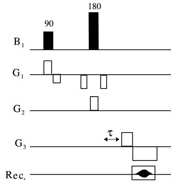
Pulse sequence for acquisition of FASTMAP linear projection field map. G1, G2 and G3 represent orthogonal oblique gradient vectors defining a given projection. As was described in Section 3.1, acquisitions must be made with two different timing parameters τ (typically τ = 0 and τ > 0). A slice selective 90° pulse brings magnetization in a given oblique slice down to the transverse plane and a 180° pulse then operates on a second slice intersecting the first slice. Readout occurs then in a direction perpendicular to both slice selection gradients.
Since there is no phase-encoding required in such columnar field-map acquisitions, each projection can be rapidly acquired. The method therefore offers an extremely fast approach to automatic shim optimization. This automated shimming approach, termed FASTMAP for Fast Automated Shimming Technique by Mapping Along Projections, was first demonstrated by Gruetter and Boesch [48], extended to include all first and second-order shims by Gruetter in 1993 [49], and optimized through various fashions in FASTERMAP [50], FLATNESS [51], and FASTESTMAP [52].
The FASTMAP method uses the spherical form of the functions (fifth column in Table 1), which transforms Eq. 51 to
| (54) |
Linear projections through the isocenter are then defined and labeled with the index j. For each linear projection, the are constant and are now denoted by . Typical definitions of for commonly utilized projections are included in Table 2. Using these definitions, a general coefficient for each order of each projection can be constructed,
| (55) |
leaving
| (56) |
Table 2.
coefficients used in FASTMAP optimization
| j | 1 | 2 | 3 | 4 | 5 | 6 | |
|---|---|---|---|---|---|---|---|
| (θ, ϕ) |
xy |
yx |
xz |
zx |
yz |
zy |
|
| Shim name | (l, m) | ||||||
| Z | (1,0) | 0 | 0 | ||||
| X | (1,1) | 0 | 0 | ||||
| Y | (1,−1) | 0 | 0 | ||||
| Z 2 | (2,0) | ||||||
| ZX | (2,1) | 0 | 0 | 0 | 0 | ||
| ZY | (2, −1) | 0 | 0 | 0 | 0 | ||
| X2 – Y2 | (2,2) | 0 | 0 | ||||
| XY | (2,−2) | 1 | −1 | 0 | 0 | 0 | 0 |
| Z 3 | (3,0) | 0 | 0 | ||||
| XZ 2 | (3,1) | 0 | 0 | ||||
| YZ 2 | (3,−1) | 0 | 0 | ||||
| Z(X2 – Y2) | (3,2) | 0 | 0 | ||||
| XYZ | (3,−2) | 0 | 0 | 0 | 0 | 0 | 0 |
| X 3 | (3,3) | 0 | 0 | ||||
| Y 3 | (3,−3) | 0 | 0 |
Magnetic field maps along each projection j can then be measured and fitted with polynomials of order l. Defining the coefficients of these polynomial regressions as yields residuals
| (57) |
A least squares formalism is then used to determine the ηlm, which can be shown [49] to produce solutions for ηlm given by
| (58) |
The projections defined in Table 2 are typically utilized. Using these projections, optimal shim settings given by evaluation of Eq. 58 are given in Table 3. If the intersection of the six utilized projections is not at the isocenter (i.e. if the volume of interest is not centered on the isocenter), the coefficients in Table 2 must be transformed according to (x,y,z) → (x + x0,y + y0,z + z0) where (x0, y0, z0) is the location of the optimization isocenter. Table 4 provides the alterations required for such considerations, where the are now labeled according to their corresponding shim labels for convenience.
Table 3.
ηlm solutions as a function of projection polynomial coefficients () for FASTMAP optimization (using the six projections specified in Table 2)
| l | 1 | 2 | 3 |
|---|---|---|---|
| m | |||
| 0 | |||
| 1 | |||
| −l | |||
| 2 | NA | ||
| −2 | NA | Undetermined | |
| 3 | NA | NA | |
| −3 | NA | NA |
Table 4.
Alterations of the in Table 2 required for projection isocenters translated off the shim set isocenter by distance (x0, y0, z0)
| l | m | W | Woff center |
|---|---|---|---|
| 1 | 0 | ||
| 1 | 1 | ||
| 1 | −1 | ||
| 2 | 0 | ||
| 2 | 1 | ||
| 2 | −1 | ||
| 2 | 2 | ||
| 2 | −2 | ||
| 3 | 0 | ||
| 3 | 1 | ||
| 3 | −1 | ||
| 3 | 2 | ||
| 3 | 3 | ||
| 3 | −3 |
In practice, it is very difficult to generate pure flm terms over extended in vivo volumes (such as the human brain). Therefore, accounting for the inevitable impurities of the shim system is critical for rapid convergence of an automated shim protocol. Particularly in human MR systems, even the most advanced coil designs possess imperfections in the individual shim field geometries. Though these imperfections can largely be decomposed into additional spherical harmonic terms, optimum coefficients calculated using the orthogonal function expansion must accordingly be modified. FASTMAP optimization can take into account downward-order impurities (e.g. first-order imperfections of a third-order shim) by calibrating the imperfections as a superposition of the other available shim terms. However the FASTMAP algorithm cannot easily account for higher order impurities (e.g. a fourth-order impurity of a second-order shim).
A means of dealing with higher-order shim imperfections in small-voxel FASTMAP applications is to locally approximate shim imperfections as lower-order terms and correspondingly alter expansion coefficients [53]. In such an approach, the shim imperfections are calibrated through field mapping measurements and fitted with higher-order spherical harmonic terms. For each implementation of FASTMAP over a reduced-volume off-center voxel, a Taylor-expansion of the interpolated imperfection around the voxel center is computed. Using these expansion coefficients, the zeroth through second-order expansion terms can be added to the pure shim calibrations to compensate for the higher-order impurities.
4.2.2. Image-based field map and least-squares optimization
FASTMAP and its derivatives ( FASTERMAP [50], FLATNESS [51], and FASTESTMAP [52]) are quick and efficient ways to homogenize ROIs defined by simple geometries using first and second-order RT shims. The utility of FASTMAP over more complicated geometries requires approaches more sophisticated than the general approach outlined here.
The improved speed of both standard workstation computers and MR imaging hardware now enable routine acquisition of three-dimensional magnetic field maps. Within the brain (where chemical shift artifacts are readily managed) field maps can easily be utilized in generalized volume shimming. Outside of the brain, chemical shift artifacts can significantly degrade the quality of field maps. The use of field maps for generalized shimming outside of the brain remains an active frontier of investigation [54,55].
Given three-dimensional field map information, a least squares shim optimization seeks to minimize the sum of squares problem,
| (59) |
where M is the number of pixels in the optimization ROI, rj is the position of the jth pixel relative to the shim set’s isocenter, N is the order of spherical harmonics used, and the flm are given in Table 1. Kim et al. [31] have presented a unique approach to solving this optimization problem. In their approach, the linear system in Eq. (59) is inverted using singular-value decomposition (SVD), which allows for regularized shim current optimization. Such a strategy can be useful to deal with shim degeneracies (an issue that will be discussed further in the explanation of dynamic shim updating methods). As reported by Wen and Jaffer [56], shim strength limitations can also be taken into account in the optimization problem framed by Eq. (59).
5. Shimming over extended volumes
The methods presented in the previous section can sufficiently homogenize the B0 distribution over small volumes and are often adequate for single-voxel spectroscopy applications. However, for many applications the aforementioned methods and hardware cannot adequately homogenize extended volumes across the whole brain.
Fig. 8 shows the effects of increasing orders of shim inclusion in the whole-brain least-squares optimization of B0 field homogeneity in the human brain at 3T. It is clear from the field-maps that low-order RT shimming leaves significant residual inhomogeneity. While there is a clear advantage of going from first (B) to second (C) order shimming, with the use of third-order shimming (D), there is significantly less improvement in homogeneity compared to second-order shimming (C).
Fig. 8.

(A) Axial MRI at B0 = 3T of two axial slices encompassing the sinus cavity region, residual inhomogeneity after (B) first order shimming, (C) with the inclusion of second-order shims, (D) with the inclusion of third-order shims.
Fig. 9 similarly shows residual field maps after global shimming of the mouse brain at 9.4T. The residual inhomogeneity here is even more severe than in the human case due to (a) the higher magnetic field strengths of small-animal MR systems and (b) the more complicated air-cavity distributions in the mouse head. Viable high-field, whole-brain, single-shot EPI images of the mouse brain have yet to be demonstrated because of this residual inhomogeneity. This severely limits the quality and temporal resolution of BOLD and DTI studies on the mouse brain.
Fig. 9.

Coronal field inhomogeneity maps of the mouse brain at 9.4T with (A) no shimming, (B) first-order shimming, (C) first and second-order shimming, and (D) first through third-order shimming.
Neuroimaging applications typically utilize whole-brain imaging strategies. In particular, DTI and fMRI seek diffusion pathways and activation patterns that characterize connectivity of neurological processes. This requires the collection of MR-based information from maximal volumetric brain data. Furthermore, both techniques require whole-brain acquisitions to be collected rapidly, thereby providing a temporal axis to measurement metrics. To address resolution requirements of this temporal axis, singleshot EPI of the whole-brain is an extremely common and useful MR protocol.
The adverse effects of B0 inhomogeneity on EPI have already been discussed in Section 2.2.1. When collecting data from across the entire brain, conventional shim technology allows for a single optimum setting of zeroth through second-order RT shims (third-order shims, when available, can sometimes provide some slight additional corrective measures). This limited shim capability has significant consequence on the quality of whole-brain, high-field EPI.
For neurological spectroscopic acquisitions, second-order FASTMAP optimization is often satisfactory for individual localized voxels. However, many applications now seek spectroscopic information from multiple regions of the brain. This also requires homogeneity optimization over much larger regions of the brain.
As previously discussed, standard RT shim construction has seen limited higher-order coil development due to constraints imposed by available bore space and the Biot-Savart law. One manner of gaining improved local homogeneity over extended volumes using existing shim coil designs is through the principle of dynamic shim updating.
5.1. Dynamic shim updating
In multi-volume acquisition protocols (such as multi-slice imaging and multi-voxel spectroscopy), the extended volume homogenizing capability of available RT shims can be improved by updating shim settings throughout the acquisitions. Such a Dynamic Shim Updating (DSU) strategy provides an optimal shim setting for each volume or slice. Here, the hardware, methods, and results of DSU as applied to whole-brain studies of the human brain are presented.
Dynamic updating of linear shim terms was first presented in the multi-voxel spectroscopy work of Ernst and Hennig in 1991 [57]. Demonstration of linear DSU capability used in multi-slice imaging was then demonstrated in 1996 by Blamire et al. [58], shortly followed by Morrell and Spielman [59]. Higher-order DSU applications to multi-slice imaging were first demonstrated by de Graaf et al. [60] on the rat brain, and then by Koch et al. [61] on the human brain. The utility of higher-order DSU in human brain imaging was also established by Zhao et al. [21] through computer simulations. Higher-order DSU application to spectroscopy on the human brain has also been presented by Koch et al. [62].
Fig. 10 illustrates the basic principle of DSU for multi-slice gradient-echo MRI. As signal is acquired from each of the slices, the settings in shim amplifiers update accordingly (where the optimum settings for each shim over each slice are determined prior to the scan). Without dedicated hardware and/or software, the shim settings would normally remain constant throughout the entire acquisition.
Fig. 10.

The principle of DSU in multi-volume acquisitions. As spins within individual slices are excited and sampled (top row), a static shim setting (middle row) would remain constant, while a dynamic shim setting (lower row) updates the currents in the shim amplifiers during each slice excitation and sampling.
DSU relies upon the ability to rapidly change settings in the shim amplifiers. Currently, many shim systems upload settings to the shim control hardware ahead of run-time via serial communication. For DSU applications, these conventional controllers have two problems associated with the serial link. First, serial communication is by design a slow protocol. Second, host computers cannot typically be relied upon to send data at a specified time. Modifying shim control hardware to locally store all slice data ahead of time can eliminate this communication bottleneck. With locally stored shim settings, it is possible for the controller to quickly retrieve shim data from memory. For example, these retrieval operations could be initiated by a real-time pulse issued by the system pulse-programmer.
Like the pulsing of imaging gradients, dynamic pulsing of shim gradients can induce significant eddy-currents in the cooled conducting structures of a MR system. It is well understood that eddy currents can be mitigated through use of actively shielded coils or standard gradient pulse pre-emphasis [63]. Full sets of actively shielded shims are not commonly available at present. Therefore, the rapid shim updating work presented here utilizes shim-pulse pre-emphasis [60,61]. The pre-emphasized spectral acquisition on the right-hand side of Fig. 11 shows the significant improvements that can be made by properly pre-emphasizing shim-change pulses. Without pre-emphasis, a water spectrum collected immediately after a significant change of the Z2 shim (A) shows multiple time-dependent frequency components that grossly distort and broaden the acquired spectrum. By applying pre-emphasis to the shim change (B) these effects are largely removed.
Fig. 11.

Water spectra collected after 25% Z2 shim changes (A) without and (B) with shim-change pre-emphasis. Reproduced from [60] with permission of Wiley-Liss, Inc., a subsidiary of John Wiley and Sons, Inc.
5.1.1. Multi-voxel MRS
Multi-voxel MRS is the principle of sampling from more than one voxel in a single TR period. It is primarily from a scan-time perspective than such an approach is more advantageous than a multiple single-voxel acquisition approach. The long TR periods and multiple averaging schemes utilized in spectroscopy often result in extended scan times. Collecting spectra from multiple voxels in the same time it takes to collect spectra from a single voxel is therefore an optimal mode of collecting spectra from multiple voxels.
Multi-voxel MRS is also more advantageous than low resolution MR spectroscopic imaging (MRSI) from a spectral quality standpoint. The localization of a multi-voxel MRS approach is far superior to a low resolution MRSI procedure, thereby resulting in reduced resonance contamination and greater SNR.
As previously mentioned, DSU’s first application was in multi-voxel spectroscopy [57]. In this pioneering work, first-order shims were set for each voxel using a potentiometer box, which is similar to the procedure used in the first multi-slice DSU approach implemented by Blamire et al. [58]. To eliminate voxel cross-excitation, collection of spectra from multiple voxels within a single TR requires oblique-localization gradients.
In demonstrating the utility of updating higher order shims in more generalized multi-voxel spectroscopy, the results of in vivo 1H MRS from four equally spaced cubic voxels of side-length 2 cm spanning the anterior to posterior midline of the human brain (see Fig. 12) are presented [62]. Voxels were constrained to a single Cartesian line (x = 0, z = 0) and localized such that the axis ran through the diagonal of each cube.
Fig. 12.

Sagittal anatomic MRI provides voxel positioning in the interleaved multi-voxel MRS acquisition. (A) Water spectra (B0 = 4T, TE = 80 ms, TR = 2.5 s, 256 averages), acquired from the four voxels using a static global shim. (B) Water spectra acquired using DSU. Linewidths of the water spectra are as indicated. (C) 1H metabolite spectra collected using DSU. Reproduced from [62] with permission of Wiley-Liss, Inc., a subsidiary of John Wiley and Sons, Inc.
Though multi-voxel spectra could be localized using either PRESS [57] or STEAM [64] localization, the results presented here utilize a modification of LASER localization [65]. Here, a slice selective SLR-90 excitation pulse [66] is followed by two pairs of spatially selective hyperbolic-secant adiabatic full-passage refocusing pulses. Unwanted coherences are removed by placing crusher gradients before and after the refocusing pulses, as well as between voxel acquisitions (in order to remove intervoxel coherences). Metabolite spectra were acquired using 6 module Gaussian-pulsed CHESS [23] water suppression preceding excitation of each voxel, TE = 80 ms, and TR = 3 s [62].
Fig. 12 demonstrates the utility of second-order DSU in multi-voxel MRS. As indicated by the linewidths of the water spectra, a static global shim setting (A) is able to adequately homogenize voxels near the global shim optimization volume (i.e. central voxels). However, for the voxel at the far anterior side of the brain, the homogeneity under the static setting is inadequate, resulting in a water linewidth of 43.2 Hz. A viable metabolite spectrum is clearly unattainable in this voxel using this shim setting. With DSU (B), its linewidth is reduced to 8.8 Hz, while the linewidths of the other three voxels also see measurable improvement. DSU-enabled metabolite spectra from all four voxels are presented in (C), where major 1H observable metabolites are clearly discernible in all voxels. This is typical of the improvements found when using dynamic versus static shim settings. Voxels in the center of the brain will likely have sufficient homogeneity under a static shim setting. However, voxels in the vicinity of either the sinus or auditory cavities will require a locally optimized shim setting.
Significant gains can be made by updating first and second-order shims on a voxel-specific basis, even when compared to updating of only first-order shims [57,64]. For example, across the four voxels presented here, the X2 – Y2 shim had optimum settings which changed by as much as 3.6 Hz/cm2 ( 25% of its available strength). Other second-order shims had similar ranges of optimum voxel-specific settings. The significant magnitude of these changes demonstrates a clear need for updating of second-order shims.
5.1.2. Multi-slice DSU
When optimizing the homogeneity of thin slices, different three-dimensional spherical harmonic shims can have the same functional form when constrained to a two-dimensional plane (i.e. the shims are degenerate). Any standard form of shim optimization will fail in the presence of significant functional shim degeneracy.
A 3D slab-based slice optimization [67] could in principle be applied by including slices on either side of the target optimization slice. However, in such a strategy (1) the shim is then optimized over the slab and not the targeted slice, and (2) the through-plane field map resolution is very low and could compromise the identification of some shim terms. The previously discussed shim-optimization approach of Kim et al. [31], also addressed the shim degeneracy problem through the use of a regularized SVD shim calculation.
The results presented here utilize an alternative to both methods, whereby two-dimensional degeneracy analysis is used to determine non-degenerate shim sets for specified imaging planes (under a thin slice approximation) [61]. The neglected shims in such an analysis are the generators of ill-conditioned matrices in the aforementioned regularized linear optimization method [31]. In combination with through-slice field map projections, such a procedure also allows for independent and robust optimization of in-plane and through-slice shim settings.
In-plane shim degeneracies for infinitesimally thin, non-oblique slices are readily determined by visual inspection. For example, when slicing in the Z direction, the only non-degenerate in-plane shims are X, Y, Z2, XY, X2 – Y2, X3, and Y3 (see Table 1 for Cartesian shim functions). The remaining shims degenerate to lower-order shims (e.g. XZ becomes a X shim).
Any arbitrary oblique slicing strategy can be represented mathematically by rotations through two Euler angles. To maintain generality we start with a reference frame (r, s, p), where r, s, and p signify the read, slice, and phase image-space coordinates. Here, (r, s, p) can be any of the six (x, y, z) gradient orientation combinations. Using the convention of Goldstein [68], rotating (r, s, p) by Euler angles θ and χ provides the rotated coordinate frame (r’, s’, p’),
| (60) |
| (61) |
| (62) |
where θ is define as the angle between r and s, and χ is uniquely determined by the chosen convention of Euler rotation.
To determine the shim selections for the entire range of θ, this analysis can be followed for a set of base angles {0, 45, 90, 135}°. Shim settings can then be used for 45° windows centered on each base angle. Though the same analysis will hold, double-oblique settings will require an extended matrix providing settings for 45° windows on each angle. Table 5 provides sets of non-degenerate shims for a number of single-oblique base angle settings.
Table 5.
Example non-degenerate shim sets based on a single oblique angle for (r, s, p) = (z, y, x) gradient orientation
| Base angle (degrees) | Shim set |
|---|---|
| 0 | X, Z, Z2, ZX, X2 – Y2, Z3, Z2X, Z(X2 – Y2), X3 |
| 45 | X, Z, Z2, ZX, ZY, Z3, Z2X, Z2Y, ZXY |
| 90 | X, Y, Z2, XY, X2 – Y2, Z2X, Z2Y, X3, Y3 |
| 135 | X, Z, Z2, ZX, ZY, Z3, Z2X, Z2Y, ZXY |
Angular ranges are 45° centered on given base angles.
The through-slice shim in a non-oblique slicing protocol is just the linear shim in the slice direction (under a thin slice assumption). However, linear through-slice shims for an oblique slicing strategy must be updated in a superposition which leaves the inplane shim field intact. We therefore must acquire a through-slice projection in the oblique-sliced direction and determine a linear trend for each slice i,
| (63) |
where rs is the through-slice coordinate. Given a normal vector to the imaging plane
| (64) |
we can then add through-slice compensation for each linear shim xj within slice i according to
| (65) |
without altering the in-plane shim. For example, a slice obliqued by 45° in the sagittal plane would have . Given a determination of η for this slice, we would then have a Y shim adjustment of and a Z shim adjustment of .
Fig. 13 illustrates significant DSU-utilized homogeneity improvement in axial slices local to the frontal sinuses and auditory cavities at B0 = 4T. Following static global shimming with up to second order shims, the global maps illustrates the severe residual inhomogeneity encountered in the frontal cortex of the brain. Field inhomogeneity of up to 150 Hz can readily be encountered a few centimeters into the brain. The field map acquired using DSU demonstrates significantly reduced frontal lobe inhomogeneity along with slight improvements near the auditory cavities. Improvements are highlighted with white arrows. These results also demonstrate that slice-specific DSU with zeroth through second-order shims cannot perfectly compensate all inhomogeneity in the human brain. The degree of improvement with DSU can also be altered with alterations in ROI definition. For instance, regions of very high inhomogeneity (such as those directly near the sinus and auditory cavities) could be omitted from slice-specific ROIs to allow the available shims to operate more selectively on lower-order inhomogeneity.
Fig. 13.

Homogeneity improvement with whole-slice optimized DSU. Field maps with (DSU) and without (global) dynamic shim changes along with slice-specific histograms for both shim settings. B0 = 4T.
5.1.2.1. MRSI
Magnetic resonance spectroscopic imaging (MRSI) is particularly vulnerable to the limitations of static whole-brain shimming [69] and is therefore an excellent platform for demonstration of DSU utility.
In conjunction with the measured B0 maps, DSU improvement is here quantified using the linewidth of N-acetyl aspartate (NAA), which was measured for all viable spectra in the presented data series.
Fig. 14 shows MRSI spectral improvements enabled through DSU. MRSI were acquired from 1-cm-thick axial slices ranging from the hippocampus to the top of the brain. A data matrix of 24 × 24 voxels over 24 × 24 cm was collected from each slice. The imaging sequence consisted of a slice-selective adiabatic inversion pulse followed by a 240-ms delay allowing for T1-nulled lipid suppression [70]. During this delay, water was suppressed by Gaussian-pulsed CHESS. Localization was accomplished with a slice-selective SLR-90 pulse and a pair of hyperbolic secant slice-selective adiabatic refocusing pulses followed by two-dimensional phase encoding gradients. Spectra were acquired with TE = 80 ms and TR = 3 s [62]. No additional outer volume suppression was used. Crushing gradients were applied before and after the refocusing pulses as well as between slices to suppress unwanted coherences.
Fig. 14.

(A) Anatomic images of MRSI slices, (B) B0 maps without DSU, (C) with DSU, (D) NAA linewidths across viable MRSI voxels with DSU, (F) without DSU, (E) spectra from indicated voxels without DSU, and (G) with DSU. (H) Provides a histogram of viable NAA linewidths across all slices with and without DSU. Images obtained at B0 = 4T. Reproduced from [62] with permission of Wiley-Liss, Inc., a subsidiary of John Wiley and Sons, Inc.
Field maps without (B) and with (C) DSU over the slice-specific ROIs utilized in shim optimization demonstrate the homogeneity improvements gained with slice-specific shim settings. [62] The impact of this homogenization on spectral quality is twofold. First, MRSI voxels distributed across slices will have reduced frequency variation, which improves water suppression. Second, narrowing of spectral linewidths will further improve water suppression and dramatically improve spectral quantification. The field maps (B–C) illuminate the former consideration, while N-acetyl-acetate linewidths without (D) and with (F) DSU quantify the latter. Selected spectra from the indicated voxels without (E) and with (G) DSU qualitatively show the overall improvement in spectral quality. Spectra are presented to demonstrate a wide range of improvements. The selected spectrum from slice 1 (in the periphery of the brain) shows tremendous improvement using DSU. Spectra from slice 4 (again near the periphery of the brain) demonstrate the improvements typical of DSU implementation. Finally, the spectra from slice 5 (in the middle of the brain, near the static-shim optimization volume) show negligible improvements using DSU. The advantages of DSU are plainly obvious. Qualitative improvements in the outer regions of the brain are presented in the selected spectra from slices 1 and 4. As seen in the B0 and NAA maps, DSU is able to dramatically reduce frequency variation and linewidths across most slices. The exception is slice 3, which is in the direct vicinity of both the auditory and sinus cavities. Due to the high-order of spatial inhomogeneity in this slice, a second-order slice specific shim setting is unable to improve significantly on the global static shim. However, this slice is an extreme case and significant improvements are made in all other slices.
5.1.2.2. EPI
As derived in Section 2.2.1, compared with conventional single-echo Cartesian imaging strategies, the phase-encoded dimension of single-shot EPI have distortion that is multiplicably exacerbated by the number of phase-encoded steps.
B0-induced distortion is often underestimated in EPI images. Distortion whereby pixels inside the brain effectively move to overlapping positions cause an intensity buildup effect that is not always easily distinguished from the underlying pixel shifts. However, this is the most common effect of image distortion. Only when pixels on the boundaries move in such a way so as to distort the outer shape of the brain is distortion obvious to the naked eye.
Such distortion is significant in high-field EPI images at typical imaging bandwidths (100–250 kHz). Using Eq. (28a), the displacement in the phase-encode direction of a given pixel can be related to the measured B0 offset at that pixel. For a 64 × 64 in-plane acquisition with a readout bandwidth of 100 kHz, an image shift of one pixel occurs in the phase-encoding direction for 24.5 Hz of B0 offset. Thus, one could effectively replace the color contrast limits in Fig. 13 with ±6 pixels to uncover how far each pixel will move in the phase-encode direction of an EPI acquisition.
Fig. 15 demonstrates improvement in geometric distortion comparing EPI images with a static global shim and second-order DSU. Improvement in the EPI images depends on slice position. The middle slices show limited improvement due to their initial (global second-order RT shim) lack of significant inhomogeneity. A number of slices show signal recovery and reduced image distortion (as indicated with yellow arrows). However, while DSU does make significant improvements, it is clear that the resulting EPI images still contain residual artifacts.
Fig. 15.

EPI images (64 × 64 in-plane pixels over 25.6 cm × 25.6 cm, 4 mm slices, B0 = 4T, TR = 2500 ms, TE = 25 ms, and readout bandwidth of 100 kHz) under static and dynamic second-order shim settings for axial slices (from left to right). Dotted lines indicate the brain contours as extracted from an undistorted FLASH acquisition (top row). Arrows designate areas of significant image quality improvement.
5.1.3. Temporal DSU
5.1.3.1. Compensation of respiration-induced B0 fluctuations
The literature has documented homogeneous and spatially varying B0 fluctuations resulting from patient respiration [71,72]. While these effects are typically low in amplitude, at B0 field strengths over 3T such physiologically induced macroscopic B0 perturbations can become problematic in highly phase-sensitive experiments.
Van Gelderen et al. [73] have developed a dynamic shimming system capable of compensating such effects in real-time. This compensation mechanism requires the introduction of two unique components to dynamic shim updating. First, the effects of respiration on the B0 (or phase-accumulation) field distribution must be measured. Second, the shim amplifiers must be triggered to update shims during scans using active measurements of the patient’s respiratory cycles. Using typical hardware available for cardiacgated acquisitions, Van Gelderen et al. calibrated and implemented such a system capable of actively compensating all zeroth through second-order respiration-induced field changes.
Fig. 16 presents the improvements in ghost reduction by compensating respiration-induced phase changes. (A) Shows images acquired without compensation. (B) Shows the images collected with temporal DSU compensation. The ghosting improvements are best visualized outside the brain region. However, ghosting does significantly impact signal intensities inside the brain as well. (C) Displays the effects of respiration on measured phase within a single imaging voxel. Both the measured phase and respiration are temporally tracked. Without temporal DSU compensation, there is a clear tracking of phase with the respiratory cycle. When temporal DSU is applied, the compensated phase has a much smaller dependence on the respiratory cycle. Though the phase modulation induced by respiration is low in amplitude, these changes can effect image ghosting. A conventional phase-correction strategy implemented in EPI uses an acquired reference scan without phase-encoding blips to measure and remove unwanted phase variations in a post-processing step. Such a correction mechanism requires extremely precise assessment of phase accumulation resulting from gradient asymmetries and induced eddy-currents. The extraneous phase modulations induced by respiration (and not accounted for in a reference-scan based correction) are easily large enough to degrade the success of such correction mechanisms.
Fig. 16.

Axial sliced gradient echo images (B0 = 7T, TE 40 ms, TR = 500 ms) without (A) and with (B) respiration-compensated dynamic shimming. (C) Temporal plots of phase measured in a single imaging voxel and respiration. Without temporal DSU, there is a clear tracking of phase with the respiratory cycle. When temporal DSU is applied, the compensated phase has a much smaller dependence on the respiratory cycle. Results courtesy of Dr. Peter van Gelderen.
Given that the incremental changes in second-order shims are very low in amplitude, this application of dynamic shim updating does not necessitate the use of higher-order shim pre-emphasis.
5.1.4. Real-time compensation of motion-induced B0 fluctuations
When a patient moves within the B0 field, the sample-induced B0 distribution will not move in a one-to-one fashion with the patient motion. Therefore, another application of DSU in the temporal regime is the compensation of shim changes induced by patient motion.
Ward et al. [74] have demonstrated that use of navigator projection field-map measurements can be applied to update linear shim terms in real-time during an EPI timeseries experiment. Patient motion can cause particularly significant temporal B0 perturbations when motion occurs in the coronal or sagittal planes. Using the field-map navigators, Ward et al. were able to insert compensating blips in the linear field gradients to compensate accumulated phase in EPI experiments. These blips could be updated on a per-image basis during timeseries acquisitions without significantly impacting on temporal resolution.
In conclusion, for multi-volume MR acquisitions DSU can enable significantly improved utility of available RT shims. Tremendous improvements in multi-voxel spectroscopy have been demonstrated with DSU, particularly when compared to static RT shimming. Temporal DSU has also been demonstrated to be extremely useful for compensation of low-order field-changes induced by patient respiration and patient motion.
Improvements in multi-slice imaging (both spectroscopic and echo-planar) are significant when DSU is utilized. However, in these investigations it is clear that even when optimized over whole individual slices, available room temperature shims remain unable to completely compensate unwanted inhomogeneity.
5.2. Alternative shimming approaches
Since there are significant physical limitations in extending RT shim technology to higher-orders, further improvements in whole-brain shimming at high static magnetic field strengths will necessarily move away from conventional mechanisms. In recent years, a number of alternative shimming measures have been proposed and demonstrated.
5.2.1. Local active shimming
Hsu et al. [75] have shown that the human oral cavity can be useful for the placement of local electromagnetic shim coils. In this approach, three independently adjustable current loops were combined to form an array of loops making different angles with respect to the axis. The shim fields produced by localized current loops are roughly dipolar in nature. However, when optimized independently, they can be combined to shape a net local-shim field on a subject-specific basis. In reference [75], a subject specific optimization procedure for use with the local shim system is also described and demonstrated.
Fig. 17 displays improvements in gained with the local shim system at 1.5T. (A) Provides a photograph of the shim assembly and its placement in the mouth relative to the brain. (B) Presents optimally shimmed field maps without (top) and with (bottom) use of the intra-oral shim assembly. (C) Demonstrates improvements in signal recovery near the sinus cavities when the local shim is utilized. Significant overall homogeneity improvements with use of the local shim coils are clear in all displayed slices.
Fig. 17.

(A) Image and anatomic location of intra-oral local active shims. (B) Field-map results of optimized local active shim use. (C) Signal-recovery in gradient-echo imaging (TE = 40 ms, 5 mm slices) with the local shim assembly. B0 = 1.5T Reproduced from [75] with permission of Wiley-Liss, Inc., a subsidiary of John Wiley and Sons, Inc.
Ohmic heating is a potential concern of this approach. While the experiments conducted at 1.5T required shim currents that did not produce appreciable temperature changes, the increased currents needed to accurately shim at 3 or 7T may need to be carefully considered. Patient comfort is also a crucial factor in the use of any oral shimming device. Wong et al. [76] have also shown initial results on an external local electromagnetic shimming approach, although such an approach has yet to be published in detailed fashion.
5.2.2. Subject-specific passive shimming
Passive shimming is an approach whereby magnetic materials are strategically placed around a sample to cancel unwanted inhomogeneity. This shimming methodology uses the induced magnetic field of the shimming material to compensate unwanted B0 heterogeneity.
Mathematically, this type of shimming is accomplished by developing the passive shim field (BPS) introduced in Eq. (45). BPS is then used in combination with the RT shim field to satisfy the shimming condition given by Eq. (46). Paramagnetic, diamagnetic, and ferromagnetic materials can all be utilized for passive shimming.
5.2.3. Intra-oral diamagnetic passive shimming
The inhomogeneity distribution generated by the sinus cavities in the human brain is roughly dipolar in shape. This general distribution geometry is created by the difference in magnetic susceptibility of air in the sinus cavities and the surrounding biological tissue. The result is a net paramagnetic dipolar effect (i.e. the field that would be generated by placement of a localized paramagnetic material in the B0 field), where the pure dipolar result is given by Eq. (19) for the field-induced external to a sphere of magnetic material. Of course, this is a very crude analysis of the problem. The local variation of sinus cavity geometries distorts this actual field geometry from that of an analytic finite dipole. However, the general lobe structure of a paramagnetic dipole can be observed near the sinus cavities of most human subjects.
Wilson et al. [77] sought to reduce the effects of this roughly dipolar field distribution by placing a highly diamagnetic material in the mouth of patients. The oral cavity is located directly underneath the sinus cavity in the direction. Therefore, the lobe of a dipole generated by placement of highly diamagnetic material in the mouth can be useful in reducing the effects of the paramagnetic dipole induced by the sinus cavities. As a diamagnetic material, Wilson et al. utilized pyrolytic-graphite (PG), which has a highly anisotropic magnetic susceptibility tensor with components χPG,⊥≈−450 ppm perpendicular to the basal plane and χPG,∥≈−85 ppm [78] parallel to the basal pane.
The construction of the diamagnetic mouth shims required fabrication of a dental mold for each patient. Such dental molds are needed to hold the graphite in place because utilization of PG’s strong susceptibility component requires positioning of the graphite in an energetically maximal configuration with respect to the B0 field. A block of pyrolytic graphite prefers to be oriented with its weak magnetic susceptibility dimension parallel to B0 and will always try to move to this preferred orientation. The forces from this anisotropic susceptibility effect are significant (though not dangerous) at 3T. It is also important to ensure that PG shim components do not move during an imaging session, as such movement could significantly compromise image quality.
An optimization procedure was developed to determine a patient-specific pyrolytic graphite oral insert from a pre-established basis set of shims [79]. This is an important consideration for human passive shimming applications, where variation across subjects is certain and significant.
Fig. 18 presents field-mapping results of intra-oral diamagnetic shimming at 3T. (A) A photograph of the graphite shim assembly. The carefully stacked construction is an important consideration due to the anisotropic magnetic susceptibility of pyrolytic graphite. Axial field maps in the top row of (B) show homogeneity attainable with available RT shim technology. The now familiar region of B0 inhomogeneity near the sinus cavity is clearly visible. Maps in the bottom row of (B) demonstrate significant improvements in homogeneity near the sinus cavity with use of the diamagnetic intra-oral shim.
Fig. 18.

(A) Photograph of the highly-ordered pyrolytic graphite shim assembly. (B) Axial magnetic field maps without and with use of an intra-oral diamagnetic passive shim. Reproduced from [77] with permission of Wiley-Liss, Inc., a subsidiary of John Wiley and Sons, Inc.
While this approach does make improvements in a number of slices, it is clear that significant inhomogeneity remains after passive shimming. Primarily in the lower slices, prominent inhomogeneity remains near the auditory and sinus cavities. Though Wilson et al. also attempted using diamagnetic ear shim-plugs, no significant homogeneity improvements were observed with their use.
5.2.4. Subject-specific ferroshimming
As previously discussed, ferroshimming is a conventional approach to shimming of the subject-independent B0 distribution within a magnet. However, there have also been approaches to ferroshimming subject-specific field distributions.
Standard copy-toner has a magnetic susceptibility close to nickel, which is ferromagnetic. Jesmanowicz et al. [80] sought to optimize printed distributions of copy toner on sheets of paper which were subsequently rolled to form ferroshim inserts. With the idea that the shims could be printed on a subject-specific basis, such a ferroshimming approach was intended to allow for robust higher-order global shimming on the human brain. This approach required the decomposition of dipolar shaped induction fields from a basis set of shim elements into spherical harmonics. Furthermore, it was assumed that the dipole moment for each induction field scales linearly with the element thickness. A least-squares linear programming solution then utilized these analytic relations of dipolar ferroshims to determine the optimum printout shim designs on a subject-specific basis. While preliminary work on this approach has been published [80], there have been no follow-up studies or rigorous assessments of the technique’s utility.
Juchem et al. [81] also developed a method of generating second-order spherical harmonic terms on a subject-specific basis using ferroshim materials. In this work, it was shown that high-amplitude second-order shim terms could be optimally produced from only a few carefully placed ferroshim (Ni–Fe permalloy) segments. Using a calibrated scaling process and optimization over targeted spherical harmonic coefficients calculated using the FASTMAP algorithm, it was demonstrated that high-amplitude second-order terms could be optimized to robustly shim the visual cortex of macaque monkeys on a subject specific basis. The primary motivation of these developments were to allow high-amplitude subject-specific second-order shimming in a high-field system (7T) equipped with relatively weak RT active shims (designed for 3T). However, the work does demonstrate that robust subject-specific passive shimming is feasible and can enhance the capabilities of available RT shims.
While all of the subject-specific passive shimming approaches discussed thus far utilize only one material for passive shimming, it has also been demonstrated that passive shimming can be accomplished using combinations of diamagnetic and paramagnetic shim elements.
5.2.5. Subject-specific diamagnetic and paramagnetic passive shimming
Given a user-defined grid for placement of shim materials, a calculation procedure to determine optimal stacks of both diamagnetic and paramagnetic shim elements at each position in the grid has been developed [82]. The accuracy of this method hinges on three approximations in the nature of the magnetic fields induced by the shim materials.
The induction fields from shim elements (or stacks of elements) at separate shim grid positions add in linear superposition.
The amplitude and shape of an induction field from a shim element is dominated by its own susceptibility and is trivially perturbed by other nearby materials with much smaller magnetic susceptibilities.
The geometric distribution of an element’s induction field does not change when elements are stacked together in a limited fashion.
The physical basis of approximations 1 and 2 is essentially the same first-order approximation to the general magnetostatic solution that has been utilized repeatedly throughout this review. Empirical measurements verifying approximations 1–3, along with the details of the following methods and results are presented in detail within reference [82].
Utilizing these approximations and given a targeted inhomogeneity distribution, the shim composition calculation can be reduced to a linear problem rapidly soluble with readily available optimization algorithms. This allows for real-time and active-adjustment of the passive shim assembly.
Due to its high surface to volume ratio, the mouse brain possesses some of the most severe magnetic field inhomogeneity found in vivo. Despite this limitation, the demand for mouse investigations in NMR has been rapidly increasing-particularly in the phenotyping of transgenic mice. Therefore, the first demonstrations of combined diamagnetic and paramagnetic passive shimming were performed on the mouse brain at 9.4T [82,83]. These shim systems used diamagnetic bismuth (Bi), paramagnetic zirconium (Zr), and paramagnetic niobium (Nb) metals as shim materials. Schenck [33] reports absolute susceptibility values for the three metals as −164, +92, and +237 ppm, respectively. Computed shim material distributions were realized on acrylic cone-shaped shim formers surrounding the mouse brains.
Fig. 19 provides field mapping diagnostics of the prototyped passive shim system in three coronal slices positioned throughout the mouse brain at 9.4T. Inhomogeneity is significantly reduced in moving from the unshimmed to the passively shimmed maps for all slices. The second-order actively shimmed map represents the best shimming alternative using previously existing technology on the utilized imaging system. Noticeable improvement is visually recognizable when comparing the passively shimmed field map to the room-temperature shimmed (RTS) field map. The required coefficients for the added inclusion of third order shims were roughly 10 times the available shim strengths, which is a common problem for RT shimming beyond second-order terms in the mouse brain at 9.4T [84].
Fig. 19.

(A) Photograph of a combined diamagnetic and paramagnetic shim assembly on the mouse brain. (B) Shim former radii and shim element positioning for two prototyped constructions. (C) Field map (B0 = 9.4T) images demonstrating the utility of the passive shim system over three coronal slices in the mouse brain, spanning a range of 3 mm. Residual field maps are shown for no shimming, active RT shimming, passive shimming with prototypes of R0 = 3.0 cm and R0 = 2.5 cm. Reproduced from [82] with permission of Elsevier.
The dramatic performance improvements of the reduced-radius shim assembly demonstrate a crucial consideration in this passive shimming approach. Compensation of higher-orders inhomogeneity with the presented shimming system benefits from the availability of steep field gradients at each grid position. Therefore, the higher-order compensating capability of the system is highly-dependent on the proximity of the shim grid to the shim volume.
The advantages of the two material passive shimming over both one metal passive shimming and low-order spherical harmonic optimization are presented in Fig. 20. Computational residual field maps from a slice near the auditory cavities are shown for both one and two metal implementations of the shim system. A field map from a computational third order room temperature shim optimized over the entire brain is also presented. The improved higher order shimming capacity of the two metal optimization over both the one-metal (Zr) and ideal third-order RT shim (using shim strengths well outside the specifications of state-of-the-art shim systems) is visually recognizable, particularly near the sinus and auditory cavities. The one-metal computation was also carried out with bismuth, which gave even poorer results.
Fig. 20.

Reduction of higher-order inhomogeneity by active and passive shimming. Residual magnetic field maps (B0 = 9.4T) near auditory air cavities are presented using (A) no shim, (B) a computational third-order RTS, (C) computational one-material (zirconium) passive shim, and (D) computational two-material passive shim. Reproduced from [82] with permission of Elsevier.
The inability of the presented passive shim system to effectively shim with one material is due to two considerations. First, the shim former geometry necessarily deviates significantly from an infinite cylindrical shape (in order to maximize proximity of the shim elements to the shim ROI). Infinite cylindrical former geometries are an assumption relied upon in other ferroshim approaches [80] to effectively generate positive and negative magnetic dipole moments with a single magnetic material. Second, the limited stack heights required to stay within the linear optimization regime restrict the efficacy of a single shim material to compensate the specified magnetic field geometries.
A significant consideration in the use of metallic passive shims is that of RF penetration and heating. Using discrete arrays of shim elements instead of continuous sheets of metal can help in alleviating this concern. Furthermore, the metals utilized in the diamagnetic/paramagnetic mouse shim system have relatively low conductivities at room temperature. B1 mapping experiments on the mouse passive shim system showed no significant RF variation with and without the use of the shim assembly. Temperature measurements were also taken directly from the shim elements to address RF heating concerns. No measurable temperature change was recorded after running a standard gradient-echo imaging sequence for 45 min with the shim system.
5.3. Future directions
5.3.1. Volume-parcellated DSU
The DSU applications demonstrated in Section 5.1 updated RT shim settings on an individual voxel (spectroscopy) or whole-slice (imaging) basis. For application to whole-brain imaging, optimization of shim settings on a whole-slice basis is the simplest and most obvious dynamic shimming pathway. However, it has been shown by Poole et al. [85] that far greater improvements can be gained with more freedom in the geometry of shim-optimized sub-volumes.
For an initial 3D field-map grid of 96 × 96 × 96 pixels, Poole et al. computationally examined whole-brain homogeneity after zeroth through second-order dynamic shimming of various volume parcellation schemes. Such parcellation schemes ranged from a single optimization volume of 96 × 96 × 96 pixels (global static shimming) to dynamic optimizations of 96 × 96 × 1 (whole-slice shimming), 96 × 12 × 8 (columnar parcellation), and 24 × 24 × 16 pixel volumes. While typical zeroth through second-order shim strengths are adequate for whole-brain or whole-slice shimming, optimization over reduced volumes can require shim currents outside of available constructions. Therefore, Poole et al. constrained their computational DSU optimization based on the efficiencies of a previously designed insertable head shim set [46].
Fig. 21 presents sample results of this investigation. Anatomic images (A) and magnetic field maps for B0 = 3T are shown for three orthogonal imaging planes using (B) static global shimming (96 × 96 × 96), whole-slice shimming (C) (96 × 96 × 1), and volume-parcellated shimming (D) (48 × 24 × 8). Residual field maps were calculated using the methods described in [85].
Fig. 21.

Computed effects of volume parcellation on the global-homogenization capabilities of DSU. Anatomic images (A) and magnetic field maps at B0 = 3T are shown for three imaging planes using (B) static global shimming (96 × 96 × 96), whole-slice shimming (C) (96 × 96 × 1), and volume-parcellated shimming (D) (48 × 24 × 8). Results courtesy of Dr. Michael Poole.
The results of this computational investigation clearly demonstrate the potential benefits of using volume parcellation in lieu of whole-slice shim optimization. The gains in global homogeneity through volume parcellation over whole-slice optimization are most noticeable in the near vicinity of the auditory and sinus cavities.
Any volume-parcellated DSU application will require an imaging sequence which is compatible with the dynamic shimming principle and possesses excitation and acquisition strategies that do not introduce extensive time penalties or reductions of SNR [85]. No currently existing imaging sequences satisfy such requirements. However, the investigations by Poole et al. show that if such a sequence could be developed, when combined with DSU, the improvements in whole-brain B0 homogeneity could be significant. Future work in this line of investigation will be focused on developing such unconventional imaging strategies.
5.3.2. Advanced passive shimming of the human brain
The human brain poses a significantly more challenging passive-shimming problem than the mouse brain for two primary reasons. First, unlike the mouse brain, most of the residual inhomogeneity in the human brain is significantly distanced from possible external shim elements. The significantly improved results of the mouse shim with only a slightly reduced shim-former diameter highlights this consideration. Second, residual targeted inhomogeneity in the human brain is highly localized. The aforementioned intra-oral diamagnetic passive shimming approach addressed this concern by placing shim elements in patients mouths. Despite the improvements gained through this approach, a more patient-friendly and freely-optimizable passive-shimming system comprised of externally located shim elements would be highly desirable. Preliminary results of combined diamagnetic and paramagnetic passive shimming on the human brain are presented here [86]. In this approach, localized diamagnetic and paramagnetic material distributions are used to effectively ‘shape’ local compensating fields and acutely target residual inhomogeneity. When such local passive shims are optimally positioned and used in combination with low-order RT shims, it is shown that residual inhomogeneity is significantly reduced compared to that after stand-alone RT shimming.
Shims were constructed of diamagnetic bismuth and paramagnetic niobium metals. Pyrolytic graphite is the only material known to be more diamagnetic than bismuth and could be used to replace bismuth in any future implementations (though the modest forces from its susceptibility anisotropy would need to be considered).
Since residual inhomogeneity in the human brain is highly localized to the sinus and auditory cavities, shim fields shaped to selectively target these regions while minimizing any adverse effects on other areas of the brain. Fig. 22 presents illustrations of auditory (A) and sinus (B) shims empirically constructed using the described shaping principles. (C) Displays and illustration of their construction relative to a human head and (D) presents a photograph of the final shim elements and their RF-coil fixation apparatus. Note that none of the shim elements are required to touch patients.
Fig. 22.

(A) Individual elements in sinus shim construction, (B) auditory shim construction (C) illustration showing full shim system, and (D) photographs of the shim construction.
Fig. 23 presents a demonstration of the principles utilized in the shaping procedure. (A) A sagittal anatomic gradient-echo MRI of the human brain. (B) Displays the residual B0 field in the human brain after second-order RT shim optimization, while (C) provides the B0 distribution after external passive shimming using only the bismuth component of the local sinus shim. Finally, (D) displays the residual B0 field after external passive shimming using the combined bismuth and niobium passive shim. Passive shim induction fields were computed using Eq. (44) while the in vivo inhomogeneity was measured using magnetic field maps.
Fig. 23.

(A) sagittal anatomic gradient-echo MRI acquisition, (B) residual B0 inhomogeneity in the brain after whole-brain optimized first and second order RT shimming at B0 = 4T, (C) computed induction field and residual inhomogeneity using a local sinus passive shim as described in Fig. 22 without use of niobium, and (D) with use of niobium. Arrows indicate regions where unwanted effects are introduced by the non-shaped shim.
When compared to the residual inhomogeneity map of the human brain after first and second order RT shims (B), it is clear that the lobe induced by either shim (C or D) would be useful in reducing residual inhomogeneity in the inferior frontal cortex of the brain. However, the bismuth-only shim (C) clearly introduces significant unwanted inhomogeneity to other regions in the frontal lobe of the brain (indicated with arrows). With the addition of niobium shaping elements, the lobe of this added dipole (inverted in sign relative to the lobe of the bismuth block) exacerbates and effectively pushes the lobe of the field induced by the bismuth block towards the positive direction. Furthermore, the lobe of the added niobium cancels the portion of the bismuth’s lobe which previously (C) had introduced unwanted effects in the superior frontal lobe of the brain. As depicted in (D), the resulting shim field selectively targets the inferior frontal cortex of the brain.
Fig. 24 presents residual inhomogeneity field-maps under second-order RT shim settings (B) and combined RT-passive shim settings (C) at 4T. Maps from three slices near the sinus and auditory cavities are presented. Improvements in residual homogeneity near the sinus and auditory cavities are clear in these maps. The field maps qualitatively demonstrate that while the constructed shim system cannot perfectly compensate unwanted inhomogeneity, it does make obvious improvements without significantly introducing additional inhomogeneity.
Fig. 24.

Field map assessment of passive-shim improvement over three axial slices (1–3) at B0 = 4T. (A) Gradient echo MRI, (B) residual inhomogeneity after zeroth through second order RT shimming, and (C) residual inhomogeneity after local passive shimming and zeroth through second-order RT shimming.
Gradient-echo images were also collected with TE = 35 ms. This is representative of TE values utilized in developing contrast in BOLD imaging at 4T. Signal recovery in these long echo-time gradient-echo images is presented Fig. 25. Signal recovery in this slice is most noticeable near both the auditory and sinus cavities.
Fig. 25.

Gradient-echo images (B0 = 4T, TE = 35 ms, slice-thickness = 5 mm, oblique angle = 20°, 128 × 128 pixels over 24 cm × 19 cm) collected without (A) and with (B) local passive shims.
Though these results demonstrate the possibility and utility of using external localized diamagnetic and paramagnetic passive shims for global shimming of the human brain, significant further investigation is required. To reach higher levels of inhomogeneity compensation, the external passive shim system could be combined with other advanced shimming approaches. For instance, Fig. 26 shows field-mapping results of combined zeroth-through second-order whole-slice optimized DSU and diamagnetic/paramagnetic passive shimming of the human brain at 4T.
Fig. 26.

Field-mapping results with utility of combined DSU and passive shimming. Axial MRI images of three slices near the auditory and sinus cavities show the position of field map traces. Residual inhomogeneity after (A) zeroth through second-order RT shimming, (B) RT and DSU shimming, (C) RT and passive shimming, and (D) RT, DSU, and passive shimming. (D) Field-map traces as indicated in MRI (A). B0 = 4T. (For interpretation of color mentioned in this figure the reader is referred to the web version of the article.)
Compared to DSU optimized over whole slices (C), it is clear that passive-shimming (D) can offer significantly more global homogenizing capability. However, when used in combination, (E) shows that DSU can be used to effectively ‘clean up’ after passive shimming to further improve inhomogeneity. More robust passive shimming will likely benefit significantly from DSU assistance. Even greater improvements and robustness to subject variations could potentially be made with the introduction of local shim coils to effectively ‘tune’ the passive shim field on a subject-specific basis.
6. Conclusion
B0 shimming remains an active field of technological development. Sections 2–4 have highlighted some of the primary considerations involved in such development. Utilizing the founding principles of magnetostatic physics, shim coil design, magnetic field mapping, and automated shim optimization, Section 5 presented the remaining challenges posed by B0 shimming of the brain. Advanced shim optimization methods addressing these challenges were further presented in Sections 5.2 and 5.3. Technological developments such as dynamic shim updating, local shim coil application, and subject-specific passive shimming were shown to hold potential for improved B0 homogeneity throughout the brain. These advancements have shown significant progress in reducing the negative consequences of B0 heterogeneity. Investigations will inevitably continue into furthering these advanced shimming capabilities and rendering them viable for general application.
Acknowledgments
The authors would like to thank Dr. Jason Hsu, Dr. Gary Glover, Dr. Peter Jezzard, Dr. Peter van Gelderen, Dr. Michael Poole, and Dr. Richard Bowtell for contributing their results to this review. Further gratitude goes to Terence Nixon, Scott McIntyre, Peter Brown and Dr. Laura Sacolick for their assistance in developing and implementing aspects of the technology presented in this review. Previously unpublished results contained in this review were funded by NIH Grants R21-CA118503 and R01-EB000473.
Glossary
- Active shimming
B0 shimming whereby sets of electromagnetic coils are used to shim in a subject-specific fashion
- Diamagnetic materials
Materials that induce magnetic fields which oppose applied fields (negative magnetic susceptibility)
- DSU: dynamic shim updating
Technique whereby RT shims are updated during an MR acquisition. Shims can be dynamically updated for specific spatial regions (slices or voxels) or in time (respiration, movement)
- EPI: echo-planar imaging
Magnetic resonance imaging technique that relies on gradient-echo refocusing to perform multiple phase-encodes on a single state (RF excitation) of transverse magnetization
- FASTMAP
Automatic RT shim optimization whereby a number of columnar field-map projections are rapidly acquired and used to calculate an optimal superposition of second-order shim coefficients
- Field map
A map of the B0 resonance frequency offsets over a specific volume. Field maps are most often measured using phase-sensitive MRI methods
- Local Active Shimming
The use of dedicated electromagnetic shim coils placed close to the patient or volume of interest to locally compensate B0 inhomogeneity on a subject-specific basis
- Magnetic induction B
The total magnetic field including inductions by free currents and material magnetism
- Magnetic susceptibility, χ
Proportionality constant relating material magnetism to the applied auxiliary field
- MRSI: MR spectroscopic imaging
MR spectroscopy technique where phase-encoding is used to spatially localize spectra
- Multi-voxel MRS
MR spectroscopy technique whereby signal is sampled from more than one voxel in a single TR period
- Paramagnetic materials
Materials that induce magnetic fields which exacerbate applied fields (positive magnetic susceptibility)
- Passive shimming
A B0 shimming approach whereby magnetic materials are strategically placed around a sample to cancel unwanted inhomogeneity
- Phase unwrapping
Technique whereby integer multiples of 2π radians are added or subtracted from phase measurements to properly determine total angular phase accumulation
- Quadrature detection
Measurement of the magnetic resonance signal whereby information on the transverse phase of precessing magnetization is recorded. Also known as I–Q or complex signal detection
- Room temperature (RT) Shimming
A form of active shimming whereby sets of electromagnetic coils representing spherical harmonic magnetic field distributions are optimized on a per-subject basis
Relaxation of transverse magnetization states caused by both conventional dipolar T2 decay and spin dephasing in macroscopic B0 field inhomogeneity
- Volume-parcellated DSU
Dynamic shimming for imaging applications where shims are not updated on a whole-slice basis, but are optimized over three-dimensional sub-volumes
References
- [1].Chen CN, Hoult DI. Biomedical Magnetic Resonance Technology. Adam Hilger; New York: 2005. [Google Scholar]
- [2].Neuberth G. 6,897,750 US Patent. 2005
- [3].Jackson JD. Classical Electrodynamics. John Wiley and Sons; New York: 1999. [Google Scholar]
- [4].Salomir R, de Senneville BD, Moonen CTW. Concepts Magn. Reson. B. 2003;19:26–34. [Google Scholar]
- [5].Marques JP, Bowtell R. Concepts Magn. Reson. B. 2005;25:65–78. [Google Scholar]
- [6].Koch KM, Papademetris X, Rothman DL, de Graaf RA. Phys. Med. Biol. 2006;51:6381–6402. doi: 10.1088/0031-9155/51/24/007. [DOI] [PubMed] [Google Scholar]
- [7].Yablonskiy DA. Magn. Reson. Med. 1998;39:417–428. doi: 10.1002/mrm.1910390312. [DOI] [PubMed] [Google Scholar]
- [8].Ogawa S, Lee TM, Nayak A, Glynn P. Magn. Reson. Med. 1990;14:68–78. doi: 10.1002/mrm.1910140108. [DOI] [PubMed] [Google Scholar]
- [9].Kwong KK, Belliveau JW, Chesler DA, Goldberg IE, Weisskoff RM, Poncelet BP, Kennedy DN, Hoppel BE, Cohen MS, Turner R, Cheng HM, Brady TJ, Rosen BR. Proc. Natl. Acad. Sci. USA. 1992;89:5675–5679. doi: 10.1073/pnas.89.12.5675. [DOI] [PMC free article] [PubMed] [Google Scholar]
- [10].Bandettini PA, Wong EC, Hinks RS, Tikofsky RS, Hyde JS. Magn. Reson. Med. 1992;25:390–397. doi: 10.1002/mrm.1910250220. [DOI] [PubMed] [Google Scholar]
- [11].Zur Y, Stokar S, Bendel P. Magn. Reson. Med. 1988:175–193. doi: 10.1002/mrm.1910060206. [DOI] [PubMed] [Google Scholar]
- [12].Bangerter NK, Hargreaves BA, Vasanawala SS, Pauly JP, Gold GE, Nishimura DG. Magn. Reson. Med. 2004:1038–1047. doi: 10.1002/mrm.20052. [DOI] [PubMed] [Google Scholar]
- [13].Yudilevich E, Stark H. IEEE Trans. Med. Imaging. 1987;6:337–345. doi: 10.1109/TMI.1987.4307852. [DOI] [PubMed] [Google Scholar]
- [14].Jezzard P, Balaban RS. Magn. Reson. Med. 1995;34:65–73. doi: 10.1002/mrm.1910340111. [DOI] [PubMed] [Google Scholar]
- [15].Andersson JL, Richter M, Richter W, Skare S, Nunes RG, Robson M, Behrens T. Proceedings of the 15th International Society on Magnetic Resonance Medicine; Kyoto, Japan. 2004.p. 87. [Google Scholar]
- [16].Bloembergen N, Purcell E, Pound R. Phys. Rev. 1948;73:679–712. [Google Scholar]
- [17].de Graaf RA, Brown PB, McIntyre S, Nixon TW, Behar KL, Rothman DL. Magn. Reson. Med. 2006;56:386–394. doi: 10.1002/mrm.20946. [DOI] [PubMed] [Google Scholar]
- [18].Michaeli S, Garwood M, Zhu X, DelaBarre L, Andersen P, Adriany G, Merkle H, Ugurbil K, Chen W. Magn. Reson. Med. 2002;47:629–633. doi: 10.1002/mrm.10135. [DOI] [PubMed] [Google Scholar]
- [19].Hahn EL. Phys. Rev. 1950;80:580–594. [Google Scholar]
- [20].Yablonskiy DA, Haacke EM. Magn. Reson. Med. 1994;32:749–763. doi: 10.1002/mrm.1910320610. [DOI] [PubMed] [Google Scholar]
- [21].Zhao Y, Anderson AW, Gore JC. J. Magn. Reson. 2005;173:10–22. doi: 10.1016/j.jmr.2004.11.009. [DOI] [PubMed] [Google Scholar]
- [22].de Graaf RA. In Vivo NMR Spectroscopy: Principles and Techniques. Wiley; New York: 1998. [Google Scholar]
- [23].Haase A, Frahm J, Hanicke W, Matthei D. Phys. Med. Biol. 1985;30:341–344. doi: 10.1088/0031-9155/30/4/008. [DOI] [PubMed] [Google Scholar]
- [24].Ugurbil K, Adriany G, Andersen P, Chen W, Garwood M, Gruetter R, Henry PG, Kim SG, Lieu H, Tkac I, Vaughan T, Moortele PFVD, Yacoub E, Zhu XH. Magn. Reson. Imaging. 2003;21:1263–1281. doi: 10.1016/j.mri.2003.08.027. [DOI] [PubMed] [Google Scholar]
- [25].Hedley M, Rosenfeld D. Magn. Reson. Med. 1992;24:171–181. doi: 10.1002/mrm.1910240120. [DOI] [PubMed] [Google Scholar]
- [26].Song SM, Napel S, Pelc NJ, Glover GH. IEEE Trans. Image Process. 1995;4:667–675. doi: 10.1109/83.382500. [DOI] [PubMed] [Google Scholar]
- [27].Chavez S, Xiang Q-S, An L. IEEE Trans. Med. Imaging. 2002;21:966–977. doi: 10.1109/TMI.2002.803106. [DOI] [PubMed] [Google Scholar]
- [28].Jenkinson M. Magn. Reson. Med. 2003;49:193–197. doi: 10.1002/mrm.10354. [DOI] [PubMed] [Google Scholar]
- [29].Cusack R, Papadakis N. Neuroimage. 2002;16:754–764. doi: 10.1006/nimg.2002.1092. [DOI] [PubMed] [Google Scholar]
- [30].Reber RJ, Wong EC, Buxton RB, Frank LR. Magn. Reson. Med. 1998;39:328–330. doi: 10.1002/mrm.1910390223. [DOI] [PubMed] [Google Scholar]
- [31].Kim D, Adalsteinsson E, Glover G, Spielman D. Magn. Reson. Med. 2002;48:715–722. doi: 10.1002/mrm.10267. [DOI] [PubMed] [Google Scholar]
- [32].Klassen LM, Menon RS. Magn. Reson. Med. 2004;51:881–887. doi: 10.1002/mrm.20094. [DOI] [PubMed] [Google Scholar]
- [33].Schenck JF. Med. Phys. 1996;23:815–850. doi: 10.1118/1.597854. [DOI] [PubMed] [Google Scholar]
- [34].Collins CM, Yang B, Yang Q, Smith M. Magn. Reson. Imaging. 2002;20:413–424. doi: 10.1016/s0730-725x(02)00507-6. [DOI] [PubMed] [Google Scholar]
- [35].Hopkins JA, Wehrli FW. Magn. Reson. Med. 1997;37:494–500. doi: 10.1002/mrm.1910370404. [DOI] [PubMed] [Google Scholar]
- [36].BioImage . Bioimaging Sciences. Yale University; New Haven, CT: 2006. [Google Scholar]
- [37].Golay MJ. Rev. Sci. Inst. 1958;29:313–315. [Google Scholar]
- [38].Romeo F, Hoult D. Magn. Reson. Med. 1982;1:44–65. doi: 10.1002/mrm.1910010107. [DOI] [PubMed] [Google Scholar]
- [39].Wong EC, Jesmanowicz A, Hyde JS. Magn. Reson. Med. 1992;21:39–48. doi: 10.1002/mrm.1910210107. [DOI] [PubMed] [Google Scholar]
- [40].Konzbul P, Svoda K. Meas. Sci. Technol. 1995;6:1116–1123. [Google Scholar]
- [41].Turner R. J. Phys. D. 1986;19:1116–1123. [Google Scholar]
- [42].Forbes LK, Crozier S. J. Phys. D. 2001;34:3447–3456. [Google Scholar]
- [43].Forbes LK, Crozier S. J. Phys. D. 2002;35:839–849. [Google Scholar]
- [44].Forbes LK, Crozier S. J. Phys. D. 2003;36:68–80. [Google Scholar]
- [45].Hoult D, Deslauriers R. J. Magn. Reson. A. 1994;108:9–20. [Google Scholar]
- [46].Poole M, Bowtell R. Proc. ESMRMB. 2006:739. [Google Scholar]
- [47].Poole M, Bowtell R. Concepts Magn. Reson. B: Magn. Reson. Eng. 2007;31B:162–175. [Google Scholar]
- [48].Gruetter R, Boesch C. J. Magn. Reson. 1992;96:323–334. [Google Scholar]
- [49].Gruetter R. Magn. Reson. Med. 1993;29:804–811. doi: 10.1002/mrm.1910290613. [DOI] [PubMed] [Google Scholar]
- [50].Shen J, Rycyna RE, Rothman DL. Magn. Reson. Med. 1997;38:834–839. doi: 10.1002/mrm.1910380521. [DOI] [PubMed] [Google Scholar]
- [51].Shen J, Rothman DL, Hetherington HP, Pan JW. Magn. Reson. Med. 1999;42:1082–1088. doi: 10.1002/(sici)1522-2594(199912)42:6<1082::aid-mrm12>3.0.co;2-g. [DOI] [PubMed] [Google Scholar]
- [52].Gruetter R, Tkac I. Magn. Reson. Med. 2000;43:319–323. doi: 10.1002/(sici)1522-2594(200002)43:2<319::aid-mrm22>3.0.co;2-1. [DOI] [PubMed] [Google Scholar]
- [53].Sacolick LI, Koch KM, Rothman DL, de Graaf RA. Proceedings of the 15th International Society on Magnetic Resonance Medicine; Berlin, Germany. 2007.p. 3433. [Google Scholar]
- [54].Maril N, Collins CM, Greenman RL, Lenkinski RE. Magn. Reson. Med. 2005;54:1139–1145. doi: 10.1002/mrm.20679. [DOI] [PubMed] [Google Scholar]
- [55].Hetherington HP, Avdievich NI, Pan JW. Proceedings of the 14th International Society on Magnetic Resonance Medicine; Seattle, WA. 2006.p. 63. [Google Scholar]
- [56].Wen H, Jaffer FA. Magn. Reson. Med. 1995;34:898–904. doi: 10.1002/mrm.1910340616. [DOI] [PMC free article] [PubMed] [Google Scholar]
- [57].Ernst T, Hennig J. Magn. Reson. Med. 1991;20:27–35. doi: 10.1002/mrm.1910200104. [DOI] [PubMed] [Google Scholar]
- [58].Blamire A, Rothman D, Nixon T. Magn. Reson. Med. 1996;36:159–165. doi: 10.1002/mrm.1910360125. [DOI] [PubMed] [Google Scholar]
- [59].Morrell G, Spielman D. Magn. Reson. Med. 1997;38:477–483. doi: 10.1002/mrm.1910380316. [DOI] [PubMed] [Google Scholar]
- [60].de Graaf RA, Brown PB, McIntyre S, Rothman DL, Nixon T. Magn. Reson. Med. 2003;49:409–416. doi: 10.1002/mrm.10404. [DOI] [PubMed] [Google Scholar]
- [61].Koch KM, McIntyre S, Nixon TM, Rothman DL, de Graaf RA. J. Magn. Reson. 2006;180:182–192. doi: 10.1016/j.jmr.2006.03.007. [DOI] [PubMed] [Google Scholar]
- [62].Koch KM, Sacolick LI, McIntyre S, Nixon TM, Rothman DL, de Graaf RA. Magn. Reson. Med. 2007;57(3):587–591. doi: 10.1002/mrm.21141. [DOI] [PubMed] [Google Scholar]
- [63].van Vaals J, Bergman A. J. Magn. Reson. 1990;90:52–70. [Google Scholar]
- [64].Theberge J, Menon RS, Williamson PC, Drost DJ. Magn. Reson. Med. 2005;53:713–718. doi: 10.1002/mrm.20350. [DOI] [PubMed] [Google Scholar]
- [65].Garwood M, DelaBarre L. J. Magn. Reson. 2001;153:155–177. doi: 10.1006/jmre.2001.2340. [DOI] [PubMed] [Google Scholar]
- [66].Pauly J, Le-Roux P, Nishimura D, Macovski A. IEEE Trans. Med. Imaging. 1991;10:53–65. doi: 10.1109/42.75611. [DOI] [PubMed] [Google Scholar]
- [67].Shen J. NMR Biomed. 2001;14:177–183. doi: 10.1002/nbm.691. [DOI] [PubMed] [Google Scholar]
- [68].Goldstein H. Classical Mechanics. Addison-Wesley; 1980. [Google Scholar]
- [69].Spielman DM, Adalsteinsson E, Lim KO. Magn. Reson. Med. 1998;40:376–382. doi: 10.1002/mrm.1910400307. [DOI] [PubMed] [Google Scholar]
- [70].Ebel A, Govindaraju V, Maudsley AA. Magn. Reson. Med. 2003;49:902–908. doi: 10.1002/mrm.10444. [DOI] [PubMed] [Google Scholar]
- [71].de Moortele PV, Pfeuffer J, Glover GH, Ugurbil KH, Hu X. Magn. Reson. Med. 2002;47:888–895. doi: 10.1002/mrm.10145. [DOI] [PubMed] [Google Scholar]
- [72].Raj D, Paley DP, Anderson AW, Kennan RP, Gore JC. Phys. Med. Biol. 2000;45:3809–3820. doi: 10.1088/0031-9155/45/12/321. [DOI] [PubMed] [Google Scholar]
- [73].van Gelderen P, de Zwart JA, Starewicz P, Hinks RS, Duyn JH. Magn. Reson. Med. 2007;57:362–368. doi: 10.1002/mrm.21136. [DOI] [PubMed] [Google Scholar]
- [74].Ward HA, Riederer SJ, Jack CF., Jr. Magn. Reson. Med. 2002;48:771–780. doi: 10.1002/mrm.10259. [DOI] [PubMed] [Google Scholar]
- [75].Hsu J, Glover G. Magn. Reson. Med. 2005;53:243–248. doi: 10.1002/mrm.20365. [DOI] [PubMed] [Google Scholar]
- [76].Wong EC, Mazaheri Y. Proceedings of the 12th Interantional Society on Magnetic Resonance Medicine; Kyoto, Japan. 2004.p. 520. [Google Scholar]
- [77].Wilson JL, Jenkinson M, Jezzard P. Magn. Reson. Med. 2002;48:906–914. doi: 10.1002/mrm.10298. [DOI] [PubMed] [Google Scholar]
- [78].Simon MD, Heflinger LO, Geim AK. Am. J. Phys. 2001;69:702. [Google Scholar]
- [79].Wilson JL, Jenkinson M, Jezzard P. Neuroimage. 2003;19:1802–1811. doi: 10.1016/s1053-8119(03)00225-8. [DOI] [PubMed] [Google Scholar]
- [80].Jesmanowicz A, Roopchansingh V, Cox RW, Starewicz P, Punchard WFB, Hyde JS. Proceedings of the 9th Interantional Society on Magnetic Resonance Medicine; Glasgow, Scotland, UK. 2001.p. 617. [Google Scholar]
- [81].Juchem C, Muller-Bierl B, Schick F, Logothetis NK, Pfueffer J. J. Magn. Reson. 2006;183:278–289. doi: 10.1016/j.jmr.2006.09.002. [DOI] [PubMed] [Google Scholar]
- [82].Koch KM, Brown PB, Rothman DL, de Graaf RA. J. Magn. Reson. 2006;182:66–74. doi: 10.1016/j.jmr.2006.06.013. [DOI] [PubMed] [Google Scholar]
- [83].Koch KM, Brown PB, Rothman DL, de Graaf RA. Proceedings of the 15th Interantional Society on Magnetic Resonance Medicine; Berlin, Germany. 2007.p. 990. [Google Scholar]
- [84].Miyasaka N, Takahashi K, Hetherington H. Magn. Reson. Med. 2006;55:198–202. doi: 10.1002/mrm.20731. [DOI] [PubMed] [Google Scholar]
- [85].Poole M, Bowtell R. MAGMA. 2008;21:31–40. doi: 10.1007/s10334-007-0102-2. [DOI] [PubMed] [Google Scholar]
- [86].Koch KM, Brown PB, Rothman DL, de Graaf RA. Proceedings of the 15th International Society on Magnetic Resonance Medicine; Berlin Germany. 2007.p. 982. [Google Scholar]