Improved free energy parameters for RNA pseudoknotted secondary structure prediction

Abstract

Accurate prediction of RNA pseudoknotted secondary structures from the base sequence is a challenging computational problem. Since prediction algorithms rely on thermodynamic energy models to identify low-energy structures, prediction accuracy relies in large part on the quality of free energy change parameters. In this work, we use our earlier constraint generation and Boltzmann likelihood parameter estimation methods to obtain new energy parameters for two energy models for secondary structures with pseudoknots, namely, the Dirks–Pierce (DP) and the Cao–Chen (CC) models. To train our parameters, and also to test their accuracy, we create a large data set of both pseudoknotted and pseudoknot-free secondary structures. In addition to structural data our training data set also includes thermodynamic data, for which experimentally determined free energy changes are available for sequences and their reference structures. When incorporated into the HotKnots prediction algorithm, our new parameters result in significantly improved secondary structure prediction on our test data set. Specifically, the prediction accuracy when using our new parameters improves from 68% to 79% for the DP model, and from 70% to 77% for the CC model.

INTRODUCTION

Many RNA structures with important functions have pseudoknots. Examples include most of the large ribosomal RNA molecules (Cannone et al. 2002) and transfer messenger RNA molecules (Andersen et al. 2006) with roles in translation, Ribonuclease P RNAs (Brown 1999) with roles in the cleavage of an extra RNA sequence on transfer RNA molecules, viral pseudoknots that induce ribosome frameshifting (Staple and Butcher 2005), and the self-cleaving Hepatitis delta virus ribozyme (Staple and Butcher 2005). Figure 1 illustrates pseudoknotted secondary structures.

FIGURE 1.

Examples of simple pseudoknots. The structures have been drawn with the visualization web service Pseudoviewer (Byun and Han 2006). (A) An H-type pseudoknot with two bands (pseudoknotted stems). The unpaired bases form a pseudoloop. (B) A non-H-type pseudoknot with a nested closed region (the leftmost stem and the attached hairpin loop).

Thermodynamics-based prediction of RNA secondary structures from the base sequence are widely used, to infer both structure and function of biological sequences, and to design sequences with novel structures. Some methods aim to find the secondary structure with minimum free energy (MFE) for the sequence, from a limited range of pseudoknotted structure types (Rivas and Eddy 1999; Dirks and Pierce 2003; Reeder and Giegerich 2004). Other algorithms use heuristic approaches (Gultyaev 1991; Ruan et al. 2004; Ren et al. 2005), which can predict a wider variety of pseudoknots, often more efficiently than dynamic programming algorithms, but are not guaranteed to find the MFE structure.

Both dynamic programming and heuristic methods use an energy model to calculate the free energy change of structures. An energy model is described by a list of structural features (such as a stacked pair); parameters, which are free energy change values, one per feature; and a function (ΔG^o) which assigns an overall free energy change to a given structure for a given sequence. The Mathews–Turner (MT) features (Mathews et al. 1999, 2004) are widely used for pseudoknot-free secondary structure prediction. The Dirks–Pierce (DP) model added pseudoknot-specific features to the MT features; their model is implemented in the NUPACK software (Dirks and Pierce 2003, 2004), and is a variant of earlier models (Gultyaev 1991; Rivas and Eddy 1999). The Cao–Chen (CC) (Cao and Chen 2006) features account in more detail for loop entropies within H-type pseudoknots (see Fig. 1). We note that an earlier model of Aalberts and Hodas (2005) also accounts for asymmetries in loop entropies that arise from differences in the major and minor grooves, using fewer features.

The accuracy of predictions depends in part on the quality of the free energy parameters. The primary goal of this paper is to provide new parameters for pseudoknotted structure prediction that can improve prediction accuracy. For pseudoknot-free parameters, there has been significant progress over three decades in optimizing parameters starting with the early work of Tinoco and others (Tinoco et al. 1973). Recently, Do et al. (2006) and Andronescu et al. (2007) introduced new methods for parameter estimation, using Boltzmann likelihood and constraint generation methods, obtaining parameters with significantly improved accuracy, compared with the parameters of Mathews et al. (1999).

In this work, we apply our constraint generation and Boltzmann likelihood (BL) methods to obtain new sets of parameters for the DP and CC energy models for pseudoknots. Toward this end, we created training data sets of reference structures, both with and without pseudoknots. Our structural data set contains over 2200 sequence–structure pairs from available databases. Our thermodynamic data set contains over 1300 sequence–structure–energy triples from the literature, where the energy is an experimentally determined free energy change of the reference structure for the given sequence. Roughly 20% of the structures in each data set are pseudoknotted.

We chose the HotKnots algorithm for pseudoknotted secondary structure prediction (Ren et al. 2005) because it was relatively simple to experiment with different energy models. This is because the HotKnots algorithm uses a modular function that returns the free energy change of a structure for a sequence. One energy function, e.g., for the DP model, can easily be replaced by a function for the CC model without changing the rest of the software. In contrast, energy parameters tend to be embedded throughout recurrences of dynamic programming algorithms, making the code difficult to change when the energy model is changed. The prediction accuracy of HotKnots compares favorably with that of other algorithms for pseudoknotted secondary structure prediction (Ren et al. 2005). Another advantage of HotKnots is that it outputs not one structure, but a small set of putative structures. Moreover, HotKnots is more efficient in both time and space requirements than the Pknots (Rivas and Eddy 1999) and NUPACK (Dirks and Pierce 2003) dynamic programming algorithms. However, a disadvantage of HotKnots is that it is not guaranteed to return the minimum free energy secondary structure. As a result, parameters that are optimized for HotKnots may not be optimized for free energy minimization algorithms.

To obtain improved parameters for pseudoknot features, we use our constraint generation method (Andronescu et al. 2007; Andronescu 2008), because it can easily be adapted for use with pseudoknots. We also use the BL parameter estimation method (Do et al. 2006; Andronescu 2008) to obtain improved parameters for the MT features without pseudoknots.

We performed several parameter training experiments to obtain new parameter sets. Training experiments varied according to whether parameters were trained in stages (with parameters for pseudoknot-free features trained first and parameters for pseudoknot features trained later) or all at the same time. Our best parameters were obtained for both the DP and CC models when the parameters for pseudoknot-free features were trained first, followed by training of the parameters for pseudoknot features. For the DP model, prediction accuracy improved from 68% to 79% compared with the initial DP parameters, and our best parameters for the CC model improved prediction from 70% to 77%.

To better understand the interplay between parameter values and prediction accuracy we analyzed the predicted structures both pre- and post-training. We show that overall, the accuracy not only of the lowest-energy (“optimal”) structure predicted by HotKnots improves, but also the accuracy of suboptimal structures reported by HotKnots. For the DP model, our analysis illustrates why simultaneously decreasing the penalty for pseudoknot initiation and increasing the penalty for pseudoknotted stems can significantly improve the accuracy of pseudoknotted structure prediction. On average, free energy changes of trained pseudoknot-free (MT) parameters are higher than free energy changes of the initial parameters, and we discuss the implications of this.

Another purpose of our analysis was to understand the degree to which the heuristic nature of HotKnots may contribute to the misprediction of structures. Using our trained parameters on short pseudoknotted structures, we found that the miss rate of HotKnots—that is, the percentage of such sequences for which the structure output by HotKnots has a higher free energy change than the reference (“true”) structure—is over 20%. As a result, the trained parameters provided in this paper may not optimize predictions of rigorous free energy minimization algorithms (which are guaranteed to have a miss rate of zero). It is likely that improvements to the HotKnots heuristic could lower the miss rate and thereby be useful in obtaining further improvements in the parameters.

HotKnots, with the old and new parameters, can be run online at http://www.rnasoft.ca. Our parameter estimation software, prediction algorithm software, data sets, and parameters are available to download from the same URL. Our software can be easily used for parameter estimation for other models or on other training sets.

RESULTS

We present results on the accuracy of HotKnots predictions with our trained parameters, and compare these results with earlier parameter sets. We also describe other properties of the parameters, such as fidelity to experimental free energy change measurements. To set the context for our results, we first briefly describe the DP and CC energy models, and then summarize our training and test datasets, our accuracy measures, and our training and prediction algorithms.

Energy models

An energy model is specified by a list of features, or structural fragments (such as a stacked pair); a vector of free energy change parameters, one per structural feature; and a free energy change function, ΔG^o. ΔG^o(x, y) is the free energy change of structure y for sequence x, with respect to the features and parameters of the model, at standard conditions (temperature 37°C and 1 M salt concentration). Typically, we have

where p is the number of features in the model, c_i is the number of times the ith feature appears in structure y, and θ_i is the parameter for feature i.

In this paper, we train (estimate) free energy change parameters for features of three models. Table 1 summarizes the type and number of features of these models; further details are provided in Materials and Methods. The MT feature set for pseudoknot-free structures was developed by Mathews et al. (1999). Our version of the DP feature set (Dirks and Pierce 2003) provides 11 additional features, such as an additive penalty for pseudoknot initiation and multiplicative penalties for base pairs and internal loops within a pseudoknotted stem. The CC model provides many additional features for H-type pseudoknots (see Fig. 1 for an example of an H-type pseudoknot). These features account for differences in entropies of loops that span the shallow groove of a helix, compared with entropies of loops that span the deep groove.5 Our version of the CC model includes coaxial stacking features within H-type pseudoknots, and uses the DP model for pseudoknots that are not H-type. Our DP energy model can be applied to arbitrarily complex structures.

TABLE 1.

The Mathews–Turner (MT), Dirks–Pierce (DP), and Cao–Chen (CC) feature sets

In Table 1, we use MT, DP, or CC to refer to the Mathews–Turner, Dirks–Pierce, and Cao–Chen feature sets, respectively. We refer to the initial settings of all DP and CC parameters (including the pseudoknot-free parameters) using DP03 and CC06, respectively. We use dp03 and cc06 when we refer to the parameters for the additional features of the corresponding model. Further parameter sets are introduced later in this section.

Data

We collected several large data sets in order to train energy parameters and to assess their accuracy. Table 2 summarizes properties of these data sets; preprocessing and other details are provided in Materials and Methods.

TABLE 2.

Statistics of the structural and thermodynamic data sets used for parameter training and testing

We collected structural data, consisting of both pseudoknotted and pseudoknot-free sequence–structure pairs from the RNA STRAND v2.0 database (Andronescu et al. 2008) and Pseudobase (van Batenburg et al. 2001). We preprocessed these data to control for length (for efficiency reasons) and quality. We then split the resulting strands into a training set, S-Train (∼80% of the total), used for parameter training on pseudoknotted energy models, and a test set, S-Test (∼20% of the total). We use S-Test to assess the accuracy of both pseudoknotted and pseudoknot-free energy models. In order to assess prediction accuracy on different types of structures, we further split S-Test into four subsets: ShPK contains short (<100 nucleotides [nt]) structures with pseudoknots; ShPKfree contains short, pseudoknot-free structures; LoPK contains long structures with pseudoknots, and LoPKfree contains long pseudoknot-free structures. In addition, in order to train parameters for pseudoknot-free features alone—i.e., parameters for the MT features—we created an additional training set, S-Train MT, which contains only pseudoknot-free structures. Since parameter estimation on pseudoknot-free structures is more efficient computationally (in large part because the SimFold pseudoknot-free secondary structure prediction software is more efficient than HotKnots, and both are used for parameter training), the average length of structures in S-Train MT is significantly larger (246 nt) than those found even in the long subset of S-Train (126 nt).

We collected a reference set of thermodynamic data, T-Train, consisting of triples with sequence, structure, and free energy changes, obtained experimentally by optical melting (Xia et al. 1998). When training parameters for the MT features, we use a subset of T-Train that has only pseudoknot-free structures, and we call this T-Train MT.

Accuracy measures

We measure the accuracy of a predicted RNA secondary structure relative to a reference secondary structure, by using the statistical measures of sensitivity and positive predictive value (PPV), and their harmonic mean, defined as follows:

When the denominators of these quantities are 0, the measure is also 0. A perfect prediction corresponds to a sensitivity and PPV of 1, and when these measures are 0, there are no base pairs in common between the predicted and reference structures. The F-measure is close to the arithmetic mean of sensitivity and PPV when the two numbers are close to each other, but is smaller when one of the numbers is close to 0, thus penalizing predictions for which the sensitivity or PPV are poor.

In addition, we measure the accuracy of the estimated free energies versus reference free energies e_i for each of the t sequence–structure–energy triples in our thermodynamic data sets. We use a root mean squared error (RMSE) as a measure of average error, for a thermodynamic data set with t triples. The closer to 0 the RMSE, the better the fit to the thermodynamic data set:

Training and prediction algorithms

We use two algorithms for parameter estimation. Our BL algorithm (Andronescu 2008) uses a maximum a posteriori approach; roughly, the goal is to find parameters that maximize the probabilities of both the structural and thermodynamic training data sets, given a prior distribution of the parameters. Our constraint generation (CG) algorithm uses constraints that guide the training of parameters, where constraints ensure that free energies of reference structures are low, relative to alternative structures for the same sequence. In our earlier work (Andronescu et al. 2007; Andronescu 2008) on parameter estimation for pseudoknot-free structures, we found that both algorithms perform comparably, in terms of the accuracy of the resulting parameters, with the BL method performing slightly better. Therefore, in this work, we use BL when training pseudoknot-free parameters. A significant advantage of the CG method, however, is that it is much easier to adapt for training of parameters for pseudoknotted features. For this reason, we chose to use CG for training of parameters for pseudoknot features in this work.

For secondary structure prediction, we use two algorithms. When the underlying model is MT for pseudoknot-free structures, we use the minimum free energy (MFE) dynamic programming method of Zuker and Stiegler (1981), as implemented in the SimFold software package (Andronescu 2003). We use the HotKnots algorithm of Ren et al. (2005) when the model is for prediction of pseudoknotted secondary structures (DP and CC).

Some details of these algorithms are given in Materials and Methods and the supplemental material, including settings of training algorithm hyperparameters and the HotKnots heuristic.

Accuracy of the initial parameters

Table 3 gives a summary of the secondary structure prediction accuracy and free energy estimation of Simfold and HotKnots on our training and testing data sets. To provide a baseline for comparison with our trained parameters in the following sections, Table 3, rows 1–3, pertains to the initial parameter sets: the MT99 parameters of Mathews et al. (1999), the DP03 parameters of Dirks and Pierce (2003), and CC06 parameters of Cao and Chen (2006). Briefly, the F-measure data on our test set S-Test shows that CC06 is best overall. CC06 does particularly well on short pseudoknotted structures, with an F-measure of 0.773 on ShPK, compared with F-measures of 0.616 for DP03 and 0.504 for MT99 on ShPK. However, the MT99 parameters provide slightly better accuracy than CC06 and DP03 on long structures and on short pseudoknot-free structures. Further details on measures of quality of the initial DP03 and CC06 parameters, including free energy values, sensitivity, and positive predictive values, are included in Supplemental Tables 1 and 2.

TABLE 3.

Summary of prediction accuracy for three models with and without pseudoknots, when using various model parameters

Training all parameters together

Next, we use our CG parameter estimation algorithm to train all of the parameters for the DP and CC features, respectively. Table 3, rows 4 and 5, shows the results. When comparing the trained DP09 parameters (Table 3, row 4) with the initial DP03 parameters (Table 3, row 2), the F-measure of the S-Test set increases by a significant 0.086. For the ShPK set with short pseudoknotted structures, the trained DP09 parameters facilitate predictions with an F-measure of 0.824, the largest F-measure for the ShPK column in Table 3. The trained CC09 parameters (Table 3, row 5) facilitate predictions that are better by 0.053 than the initial CC06 parameters on S-Test. In addition, the RMSE values are significantly lower than those obtained with the initial parameters, and the RMSE values for the newly trained CC09 parameters (Table 3, row 5) are the best for the column.

These results demonstrate that by using well-designed parameter estimation algorithms and large and diverse training sets, we obtain significantly better accuracy (for example, the F-measure increases by 0.086 and 0.053 for the DP and CC models, respectively), when averaged on S-Test.

Training the pseudoknot-free parameters

Next, using the BL algorithm, we trained the parameters of the MT model on the training sets S-Train MT and T-Train MT that do not include pseudoknots (Andronescu 2008). We denote the parameters obtained as MT09, see Table 3, row 6. The predictions of the pseudoknot-free sets are significantly more accurate than in previous rows of Table 3. Therefore, since BL was previously shown to perform slightly better than CG, and since the structures of the training set S-Train are longer than those of the training set S-Train PK, in the following experiments we fix the pseudoknot-free parameters to the MT09 parameter set (Table 3, row 6).

Table 3, rows 7 and 8, shows the performances of the DP and CC models, respectively, with the newly trained MT09 parameters and the initial dp03 and cc06 parameters. The F-measure of the longer structures with pseudoknots is the same as for the MT09 parameters, and the F-measure is also the same on both short and long pseudoknot-free structures. However, for the short structures with pseudoknots, the F-measures for the DP parameters in Table 3, row 7, are significantly lower than the corresponding DP parameters in Table 3, rows 2 and 4; and, similarly, the F-measures for the CC parameters in Table 3, row 8, are significantly lower than the corresponding CC parameters in Table 3, rows 3 and 5. We discuss some reasons for this in the Discussion section.

Training the pseudoknot-free and the pseudoknot parameters separately

We trained the DP and CC parameters while keeping the pseudoknot-free parameters fixed to the MT09 parameters obtained in the previous section.

Table 3, row 9, shows the results for the DP model. We obtain an improvement of 0.109 from the initial DP03 parameters (Table 3, row 2), when averaged on the entire S-Test. The average F-measures for S-Train and S-Test are the highest for the corresponding columns in Table 3. Compared with the initial DP03 parameters (Table 3, row 2), every set is predicted significantly more accurately. When compared with the parameters trained altogether (Table 3, row 4), all of the sets are predicted more accurately (particularly the long pseudoknot-free structures), except for the ShPK set, which has an F-measure lower by only 0.007. We denote this parameter set as DP09; this is the most accurate parameter set we obtained for the DP model, and the most accurate overall, when averaged on S-Test.

Table 3, row 10, shows the results for the CC model, when the pseudoknot-free parameters are fixed to the MT09 parameters and the DP additional parameters are fixed to the dp09 parameters just obtained. When measured on the entire test set S-Test, these parameters, which we denote as CC09, are the best overall for the CC model. The average F-measure for each individual test set is comparable with the F-measure obtained with the DP09 parameters (Table 3, row 9), except for the ShPK set, in which the F-measure is poorer by 0.075.

Therefore, although the initial CC06 parameters give better F-measures than the initial DP parameters (particularly for the ShPK test set), we have obtained slightly more accurate predictions for the newly trained DP09 parameters than for the CC09 parameters. This does not necessarily mean the features of the DP model are better. It is possible that the large number of additional CC features, together with coaxial stacking features, make it infeasible to train them accurately, given the limited available structural and thermodynamic data. Feature relationships could be used, as proposed by Andronescu (2008). In addition, the CC model of Cao and Chen (2006) does not cover all possible H-type pseudoknots. The more recent CC model (Cao and Chen 2009) could be used in the future. Supplemental Tables 1 and 2 provide further details on the accuracy of the DP09 and CC09 parameters.

Correlation of initial versus trained parameter values

We examined the correlations between the values, i.e., free energy changes, of the trained parameters versus the initial parameters for each of the MT, CC, and DP feature sets. Figure 2A shows the MT09 parameters versus the initial MT99 parameters, with a correlation coefficient of 0.79.

FIGURE 2.

Trained parameters versus initial parameters for the MT and CC models. (A) MT model, correlation coefficient 0.786. All parameters appear in the training data. (B) CC entropy parameters, correlation coefficient 0.983. Only 188 out of 258 parameters appear in the training data. (C) Coaxial stacking free energy change parameters, correlation coefficient 0.718. Only 166 out of 288 parameters appear in the training data.

The trained loop entropy parameters of the CC model (which comprise 258 of the full set of 920 CC09 parameters—see Table 1) versus the initial loop entropy parameters are shown in Figure 2B. These parameters are very well correlated (correlation coefficient 0.98). Thus, our parameter training methods selected parameters very close to CC initial estimates (which were obtained using statistical mechanics simulations). Figure 2C shows the trained coaxial stacking parameters (which comprise 288 of the full set of 920 CC09 parameters) versus the initial coaxial parameters. The correlation coefficient of 0.72 is slightly lower than that (0.79) for the MT parameters, most likely because the number of coaxial stacking parameters is large and we have limited training data.

For the 11 DP features for pseudoknots, Table 6 (see below) provides the initial and trained values. Parameters for two of the features that penalize initiation of pseudoknots are significantly lower for the trained parameters, compared with the initial parameters, and the penalty for adding bands (pseudoknotted stems) is higher. The remaining eight parameter values are very similar for trained and untrained data. In the next section, we show how these changes improve the prediction quality of the DP model.

TABLE 6.

DP pseudoknot features and the dp03 and dp09 parameters

DISCUSSION

From the Results section, it is apparent that the trained CC09 and DP09 parameters show large improvements over the initial versions. In the following sections, we will discuss some of the reasons for these improvements and the trends that we have observed in structure predictions. In discussing these trends, we note that HotKnots outputs several possible structures for a given input, ranked by their free energy change. We refer to the output structure with the lowest free energy as the optimal structure and the remaining structures as suboptimal structures. Note that since HotKnots is a heuristic algorithm, the optimal predicted structure may not be the MFE structure. Of all structures (both optimal and suboptimal) predicted by HotKnots for a given input, we call that structure with the best F-measure the best suboptimal structure. Table 4 provides a useful summary of our discussion, and is referred to throughout this section.

TABLE 4.

Statistics of initial and trained DP and CC parameter sets on our test sets

The CC09 and DP09 parameters improve on CC06 and DP03, with respect to both optimal and suboptimal structure predictions

Before parameter estimation, the CC model (CC06) produces better predictions than the DP model (DP03), on average, and especially for short pseudoknotted structures. First, the average F-measure of optimal and suboptimal predictions is slightly higher on S-Test for CC06 than for DP03 (see Fig. 3). The most striking difference between CC06 and DP03 is on the ShPK structures in S-Test, for which the structures predicted by CC06 have a much higher average F-measure than those predicted by DP03 (0.77 versus 0.62), and for which the best suboptimal predicted by CC06 has a somewhat higher F-measure than that predicted by DP03 (0.91 versus 0.88). This is not surprising, as CC06 handles H-type pseudoknots more rigorously than DP03. Second, on reference pseudoknotted structures, DP03 predictions are mainly pseudoknot-free (67.9% of predictions on ShPK structures and 80.0% of predictions on LoPK structures are pseudoknot free) with only one stem being reproduced correctly or almost correctly, and an adjacent pseudoknot-free structure sometimes added. CC predictions, on the other hand, are more dominated by pseudoknots (only 30.8% of predictions on ShPK structures and 70.0% of predictions on LoPK structures are pseudoknot-free). Finally, on the ShPK data set, if the optimal CC06 prediction is not the reference structure, but the reference structure is found among its suboptimals, then it is ranked higher among its suboptimals than in DP03. On average, the best CC06 suboptimal ranks at 1.54, while the best DP03 suboptimal ranks at 2.10 (Table 4).

FIGURE 3.

F-measures for every sequence in S-Test, as predicted by the initial DP parameters (DP03), the newly trained DP parameters (DP09), the initial CC parameters (CC06), and the newly trained CC parameters (CC09). (A) DP03 versus DP09. Correlation coefficient 0.542. DP09 is better than DP03 in 49% of the cases, equal in 34% of the cases, and worse in 17% of the cases. (B) CC06 versus CC09. Correlation coefficient 0.552. CC09 is better than CC06 in 46% of the cases, equal in 35% of the cases, and worse in 20% of the cases. (C) CC09 versus DP09. Correlation coefficient 0.921. DP09 is better than CC09 in 5% of the cases, equal in 93% of the cases, and worse in 2% of the cases.

After parameter estimation, DP09 is, on average, slightly better than CC09 on S-Test, in terms of the optimal structure F-measure, and is comparable in terms of the best suboptimal F-measure. On the ShPK structures, DP09 does better than CC09 on both of these measures. Despite often finding all of the DP09 structures among its own suboptimals, the CC09 model reverses the rank of better predictions with poorer predictions among its suboptimals compared with DP.

Higher sensitivity for pseudoknots comes at a cost of slight increase of prediction of spurious pseudoknots

Before parameter estimation, especially for reference structures that are short H-type pseudoknots, the DP model often predicts a pseudoknot-free structure containing one stem of the reference pseudoknot, whereas the CC model is able to identify the whole pseudoknot. In the ShPK structures of S-Test, 37.2% of the optimal structures are those where DP03 predictions are pseudoknot-free, but CC06 predictions are pseudoknotted. Parameter estimation improves the DP model in allowing it to predict more pseudoknots where appropriate (higher sensitivity), with only a slight increase in the number of spurious pseudoknots.

To illustrate the higher sensitivity, we note that on the ShPK test set (reference pseudoknots), 32.1% of optimal DP03 predictions are pseudoknotted, whereas 79.5% of optimal DP09 predictions are pseudoknotted (Table 4). Additionally, there are no test cases in which DP03 predicts a pseudoknot, but DP09 does not. This improvement is likely due to the fact that starting pseudoknots becomes favorable with the new parameters (−1.38 kcal/mol versus 9.6 kcal/mol for the pseudoknot initiation penalty) (see Table 6 below).

Table 4 shows that the percentage of spurious pseudoknots in ShPKfree increases from 2.3% for DP03 to 6.5% for DP09, but decreases from 12.3% for CC06 to 8% for CC09 (a similar trend, but to a lesser extent, is seen for the LoPKfree data set). Although the increase in sensitivity of DP09 comes at a slight cost of the increase in the predicted spurious pseudoknots, the percentage is lower than the percentage for CC09.

DP09 and CC09 predict fewer false positives and false negatives for complex pseudoknots than DP03 and CC06, respectively

Compared with the DP09 parameters, predictions with the DP03 parameters include more unnecessarily complex pseudoknotted structures. To quantify this, we partition the pseudoknotted structures into two types. We use the notion of structure density (see Jabbari et al. 2008) for this purpose. Roughly, the density of a structure is the maximum number of mutually overlapping bands (i.e., pseudoknotted stems) in the structure. For example, the structure shown in Figure 4A has density 2, while the structure shown in Figure 4B has density 3. Structures that have a density of, at most, 2 include H-type pseudoknots, kissing hairpins, and pseudoknot-free structures. We consider structures that have density 3 or greater to be “complex.”

FIGURE 4.

Comparison of DP03 and DP09 predictions on the GaLV pseudoknot. (A) Reference structure, which is also the structure predicted using the DP09 parameters. (B) Structure predicted using the DP03 parameters. This structure is unnecessarily complex, and has an F-measure of 0.471.

First, consider sequences in S-Test where the reference structure has density 2 or less, but DP03 and DP09 optimal predictions have density 3 or density 4 (density-4 structures are the highest density structures in S-Test). As shown in Table 4, all of the sequences with a density >2 in the optimally predicted structures using DP03 and DP09 had a density ≤2 in the reference structure. The number of predicted structures with a density >2 decreases from 18 in DP03 to 9 in DP09, indicating that the initial DP03 parameters are much more likely than the DP09 parameters to falsely predict unnecessarily complex pseudoknotted structures. The DP03 structures suffer because of a high pseudoknot initiation penalty: when a pseudoknot is introduced, DP03 is more likely to add more bands (as band penalty is low and the reward of the added stem can be high), and thus more complexity, to compensate for the high positive free energy change of pseudoknot initiation.

A simple example of this phenomenon is the GaLV sequence (van Batenburg et al. 2001), for which the optimal model predictions are shown in Figure 4. The DP09 prediction is 100% accurate, whereas the DP03 prediction is a poorly predicted pseudoknot with density 3.

To check that the DP09 model does not falsely predict simpler pseudoknots even in cases where the reference structure is complex, we consider the two cases in S-Test that have complex reference structures: Ec_alpha (density 3) and PDB_00716 (density 4). For Ec_alpha, the DP03 optimal prediction (F-measure 0.361) is a pseudoknot-free structure matching just part of one stem to the reference structure, while the DP09 optimal prediction (F-measure 0.633) is a kissing hairpin matching parts of two stems to the reference structure, with more base pairs added than necessary. In addition, the four DP03 suboptimal predictions are all pseudoknot-free, whereas for DP09, the 15 suboptimals have better F-measures on average (0.514 versus 0.302), with the best suboptimal (F-measure 0.776), predicted as a similar density-3 structure with one stem matching the reference structure exactly, and having either too many or too few base pairs for the other two stems. The DP09 suboptimals also include two other structures of density 3 with shifted stems and an adjacent pseudoknot-free region. Thus, for Ec_alpha, DP09 does well at predicting pseudoknots of the expected complexity.

The difference for PDB_00716 is not as striking. The optimal DP03 and DP09 predictions both have 0 F-measures, even though the DP09 prediction is an H-type pseudoknot, whereas the DP03 prediction is pseudoknot free. The suboptimal structures differentiate the models further. All but one of the five DP03 suboptimal predictions are pseudoknot-free with a best suboptimal F-measure of 0.326 (corresponding to a pseudoknot-free structure), while, again, the DP09 suboptimals are more promising: nine out of 19 are density-2 structures, one has density 4, the rest are pseudoknot-free, and the best suboptimal (F-measure 0.930) matches a nested pseudoknot-free region and two of the reference stems exactly, except for an extra base pair. Although we cannot confidently generalize from only two test cases, this suggests that if suboptimals are considered, DP09 can also produce high-complexity pseudoknots where expected.

The discussion above also holds for the CC models. As shown in Table 4, the number of predicted structures with a density >2 decreases from 20 (in CC06) to 9 (in CC09); again indicating that the initial parameters are more likely than the CC09 parameters to falsely predict unnecessarily complex pseudoknotted structures.

In terms of falsely predicting simpler pseudoknots, we again consider the Ec_alpha and PDB_00716 pseudoknots. CC09 predicts the Ec_alpha pseudoknot complexity better than CC06, generating the optimal structure and 38.5% of suboptimals as pseudoknot-free with a best F-measure of 0.731. In comparison, all of the CC06 predictions are pseudoknot-free with a best F-measure of only 0.393. The PDB_00716 pseudoknot does not show the same striking difference. CC09 does predict 43.8% compared with 33% of CC06 suboptimals as pseudoknotted. However, the best suboptimal F-measure is 0.564 for CC09, compared with 0.681 for CC06.

CC09 performs better than CC06 on average, at the cost of slightly decreased accuracy on short pseudoknotted structures

On S-Test, the CC09 model achieves a higher average F-measure on the optimal predictions than CC06. In fact, on all structures except ShPK, CC09 performs much better than CC06 (with 9%, 11%, and 5% increases) (as shown in Tables 3,4) and does only 3% worse than CC06 on ShPK. One reason for the relatively poor performance of CC09 on ShPK may be that the new parameters often force CC09 energies to be much higher than CC06 energies for pseudoknotted structures. (We compare free energy changes of CC06 and CC09 further in an upcoming section.) The HIV-1-RT-1-7 pseudoknot (illustrated in Supplemental Fig. 1) is an example of where CC09 fails to predict a pseudoknot. The CC06 prediction is perfect, whereas the CC09 prediction F-measure drops significantly, now forming a pseudoknot-free structure that matches only one stem of the reference H-type pseudoknot (and adding the second stem would increase the free energy change). Of all 22 structures in the ShPK test set for which the CC09 F-measure is worse than the CC06 F-measure, seven (31.8%) are structures in which the CC09 prediction is pseudoknot-free, whereas the CC06 prediction is pseudoknotted. Rather, the majority of cases (9/22 = 40.9%) are structures where both models predict pseudoknots, but CC09 shifts stems or adds/misses base pairs. The remainders are cases where both are pseudoknot-free or CC09 predicts a pseudoknot that is less accurate than the CC06 pseudoknot-free prediction.

Use of the heuristic prediction algorithm may adversely affect model results

Because of its heuristic nature, HotKnots may not find the MFE structure as its optimal prediction. An example of this phenomenon is the HIV-1-RT-2-10 pseudoknot (shown in Supplemental Fig. 2) with the CC and DP predictions before and after parameter estimation. For both models, before and after parameter estimation, the reference structure is not predicted as the optimal prediction even though the energy of the reference structure is less than the energy of all structures predicted by HotKnots.

To obtain a lower bound on the number of times our predictions suffer from this limitation of HotKnots, we can compute the percentage of sequences in a given data set for which the energy of the reference structure is less than the energy of the optimal model prediction. We call this percentage the miss rate of HotKnots on the data set. On ShPK, the miss rate is 3.8% for DP03, 24.4% for DP09, 16.7% for CC06, and 23.1% for CC09 (see Table 4). The miss rate is much lower (mostly 0%) for the other test sets, as shown in Table 4. Thus, HotKnots' miss rate is worse on the trained parameters than on the initial parameters.

This arises in part because the DP03 and CC06 parameters cause the reference structures to have high free energy changes relative to alternative structures. For example, with the DP03 parameters, most of the pseudoknotted structures in ShPK have higher free energy changes than the MFE pseudoknot-free structures. Since the MFE pseudoknot-free secondary structure is always considered by HotKnots, HotKnots always avoids increasing its miss rate in such cases. With the new DP09 parameters, it is harder for HotKnots to find a structure with a free energy change less than or equal to the reference structure—since the MFE pseudoknot-free structure is less likely to suffice for this purpose. HotKnots uses a number of thresholds to make decisions (for details, see Ren et al. 2005). These thresholds were set based on the DP03 parameters. We expect that different thresholds would be more appropriate for the revised energy parameters, and could reduce the miss rates further. For example, when generating an initial list of hotspots, HotKnots uses an extra penalty for including bulge loops of size 1 or 1 × 1 internal loops. These penalties were chosen in a fairly ad hoc manner, and optimized to work well with the DP03 model. With new free energy parameters, these penalties may not apply as well.

It is likely that improvements to the HotKnots heuristic could lower the miss rate and thereby be useful in obtaining further improvements in the parameters, either for HotKnots itself or for minimum free energy prediction programs. An important caveat, highlighted by the low miss rate of HotKnots on DP03, is that a low miss rate is not enough on its own to guarantee high prediction accuracy. Rather, the energy parameters are key because HotKnots outputs the lowest-energy structures it finds for a given sequence. To what degree HotKnots can be improved (with the current or even better parameters) by reducing its miss rate is an interesting direction for future work.

Energies for post-parameter estimation structures are higher than for pre-parameter estimation structures

In this section, we describe the effect of the new parameters on the free energy changes of structures. We first discuss the RMSE values shown in Table 3. On T-Train PK, the initial DP03 and CC06 parameters yield RMSE values of 3.39 and 6.40 kcal/mol, respectively. Our new DP09 parameters yield a slightly worse RMSE value than initially (3.53 versus 3.39), but the CC09 parameters yield a much better RMSE (2.97 versus 6.40). All of the RMSE values on T-Train PK are worse than the RMSE values obtained for the pseudoknot-free structures in T-Train PKfree (which are around 1.0 kcal/mol). This suggests that the sets of features and parameters for pseudoknots are currently much harder to estimate than for pseudoknot-free structures. This is likely because there is much less available data with pseudoknots; we have only 22 pseudoknotted structures in T-Train PK, compared with 1300 structures in T-Train PKfree.

As an example, we consider the human telomerase RNA pseudoknot (see Fig. 5) and two mutants, which are part of our T-Train PK data set. The free energy changes of these structures at 37°C and 1 M NaCl were determined experimentally by Theimer et al. (2005). Table 5 shows the experimental and predicted free energy changes for the reference structures, and for the initial and trained DP and CC parameters. While the wild-type free energy is approximated more poorly with the new parameters, the approximation is better for the mutant variants.

FIGURE 5.

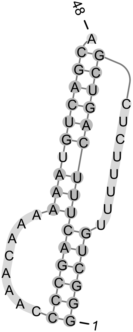
The human telomerase RNA pseudoknot (wild type).

TABLE 5.

Experimental and predicted free energies (kcal/mol) for the human telomerase RNA pseudoknot (wild type and two mutants)

An important trend in free energy changes can be observed from Figure 2. In Figure 2A, which shows the correlation between MT99 and MT09 energies, there are more points above the diagonal than below. Thus, the structure energies for MT09 tend to be higher than energies for MT99. The MT features contribute more to structure energy changes than do the CC or DP features, especially for long sequences. We therefore expect post-training energies to be higher than pre-training energies. This is confirmed by the average free energy changes of reference structures in S-Test: the CC model energies increase from −19.92 kcal/mol pre-parameter estimation to −12.80 kcal/mol post-parameter estimation, and DP model energies similarly increase from −16.95 to −12.80 kcal/mol. The correlation plots in Supplemental Figure 3 provide further evidence.

Figure 2B shows that the trained CC09 loop entropy parameters are on average lower than the CC06 loop entropy parameters. This may be a consequence of the higher MT09 parameters: in order for pseudoknots to be predicted, given the MT09 parameters, it may be necessary for loop entropies in pseudoknots to be more favorable. Similarly, the higher MT09 parameters likely have the effect of depressing the trained pseudoknot initiation penalty for the dp09 parameters. As further evidence of this, we note that with the MT09 + dp03 parameters, no pseudoknots are predicted at all on sequences in ShPK. We believe that this is because the high pseudoknot initiation penalties in dp03, together with the relatively high MT09 parameters, cause pseudoknots to be energetically unfavorable.

Conclusions

In summary, we have developed two new parameter sets, DP09 and CC09, for pseudoknotted secondary structure prediction with HotKnots. On our test set (which has 446 sequences with an average length of 74 and their reference structures) our new parameters provide significantly better structure prediction accuracy than the initial DP03 and CC06 parameter sets, resulting in 11% and 7% improvement in prediction accuracy, respectively. For the DP model, the improved accuracy results, in part, from higher sensitivity in prediction of short (H-type) pseudoknotted structures, with a corresponding decrease in prediction of pseudoknot-free structures or unnecessarily complex pseudoknots when the reference structure is H-type. In contrast, the CC09 parameters are somewhat poorer than the CC06 parameters in prediction of short pseudoknots, but improve prediction accuracy on other test data.

Training the DP parameters on training sets that did not contain specific families of pseudoknotted RNAs (specifically, in one experiment we excluded all 62 transfer messenger RNAs, and in another we excluded all 181 RNase P RNA molecules), resulted in comparable prediction accuracy on our test sets: <2% difference for ShPK, and <1% difference for the remaining three sets, when compared with DP09. This suggests that our new parameters are likely to perform well on RNA families that have not been used for training.

Besides prediction accuracy, another measure of quality of energy parameters is the degree to which they accurately predict experimentally determined energies. With respect to a RMSE measure, the CC09 parameters predict energies that are closest to experimentally determined energies. We also found that on our test data, the trained parameter sets predict energies that are higher, on average, than the initial sets. Finally, we note that HotKnots has a higher miss rate with the new parameters than with the initial parameters. Further improvements in prediction accuracy may be possible by changing HotKnots to reduce its miss rate.

MATERIALS AND METHODS

Data sets

Here, we describe the details of the structural and thermodynamic sets.

Structural data

We have collected structural data, that is, reference sequence–structure pairs, from three sources: (1) The first set, S1, includes the data used for evaluation of pseudoknotted prediction algorithms (Ren et al. 2005; Jabbari et al. 2007). This set has 89 structures, with an average length of 62 nt. (2) The second set, S2, contains the sequences and secondary structures included in Pseudobase (van Batenburg et al. 2001), from which we eliminated 15 structures that are already in S1. Pseudobase contains a collection of RNA fragments with pseudoknots, including a large number of viral RNA fragments, and some ribosomal RNAs, messenger RNAs, transfer messenger RNAs, ribozymes, and aptamers. S2 contains 228 molecules with an average length of 46.6 nt. (3) The third set, S3, was created using the database RNA STRAND v2.0 (Andronescu et al. 2008), and contains 1936 structures with an average length of 78 nt (we eliminated all structures that were already in S1 and S2). To obtain the S3 set from the full collection RNA STRAND v2.0, we applied the following selection and preprocessing steps (Andronescu 2008):

1. We eliminated any structures formed from more than one strand, as well as structures for sequences <10 nt long. Modified nucleotides (e.g., in tRNA structures) were replaced by the original nucleotide before modification. For each hairpin loop with less than three unpaired nucleotides, we opened up (removed) one or two base pairs, such that the number of free bases in a hairpin loop is at least three.

2. We removed noncanonical base pairs (i.e., AA, AC, AG, CC, CU, GG, and UU). We replaced unknown nucleotides (denoted by N) that are in base pairs by the Watson–Crick complement of its partner in the base pair. Unknown nucleotides that were unpaired, and for which there were no base pairs between them and the 5′ or 3′ end of the molecule, were removed by shortening the ends of the molecule. In all other cases where structures contained unknown nucleotides, we eliminated the structures from the set.

3. We eliminated all structures that contained a long loop, since we were concerned that these regions were poorly annotated. Specifically, we eliminated structures containing hairpin loops, bulges, and internal loops with lengths >50, and multiloops with lengths >100. We shortened very long structures, such that the maximum number of nucleotides per structure is 200, and we split the structures at external loops, keeping folding domains (i.e., external loop branches) intact. In addition, since most of the transfer messenger RNAs are longer than 200 nt, we split the structure at the large multiloop.

4. We eliminated isolated base pairs (i.e., those forming a band with no other base pairs) from structures, since these would be considered tertiary, rather than secondary structure features. We eliminated duplicated sequences and their corresponding secondary structures, such that all the sequences in the final set are pair-wise distinct.

5. We combined S2 and ∼80% of S3 to obtain the set S-Train and use it for training. Then, we combined S1 and the remaining ∼20% of S3 to obtain S-Test and use it for testing (see Table 2).

6. Additionally, we created a separate training set called S-Train MT to train pseudoknot-free parameters only. This was created in the same way as the set S3 described above, except the maximum sequence length was 700 nt, and the structures that had long pseudoknots were eliminated (including transfer messenger RNAs, RNase P RNAs, group I introns, and hepatitis delta virus ribozymes). If any of the remaining structures contained pseudoknotted base pairs, we opened up these pairs to obtain pseudoknot-free structures.

Thermodynamic data

We have collected data from 31 thermodynamic experiments on structures with and without pseudoknots described in five studies (Puglisi et al. 1988; Wyatt et al. 1990; Qiu et al. 1996; Theimer et al. 2003, 2005), and we have added these experiments to the thermodynamic set T-Full (Andronescu 2008), to obtain the thermodynamic set T-Train. Twenty-two of the 31 added experiments contain pseudoknots.6 Table 2 gives the statistics of T-Train.

Energy models

In this section, we describe details of the MT, DP, and CC feature sets and energy functions, and provide some background on the initial parameters for these feature sets. Supplemental Figures 4–6 provide concrete examples.

Mathews–Turner (MT) model

Our version of the MT feature set (Mathews et al. 1999) is as implemented in the SimFold software (see also Andronescu 2003). There are 363 features overall, including features for hairpin loops (such as terminal mismatches and length), internal loops (with distinct features for small loops, such as 1 × 1 loops, as well as terminal mismatches, a length penalty, and an asymmetry penalty), multiloops (initiation, branch, and unpaired base penalties), and external loops. We include a penalty for all closing AU pairs, including those in pseudoknotted stems, but do not include features for coaxial stacking.

The MT99 parameters were provided by Mathews et al. (1999); they were inferred from available data using linear regression and genetic algorithms. The MT free energy change function is exactly as given in Equation 1.

Dirks–Pierce (DP) model

The DP feature set includes all of the MT features, along with additional features for pseudoknots, which are summarized in Table 6. We use the following notation given by Rastegari and Condon (2007) to describe the features for the pseudoknots of the DP model. If bases are numbered from the 5′ end, starting at 1, then base pair i.j is pseudoknotted if it crosses at least one other base pair i′.j′; that is, if i < i′ < j < j′. A band is a maximal collection of pseudoknotted base pairs, all of which cross the same base pairs. Base pairs in a band are nested, with an internal loop or multiloop between successive base pairs. These internal loops and multiloops span the band. Unpaired bases in a pseudoknot are those bases that are interspersed between (but not within) connected bands, and are not in nested substructures. For example, in Figure 1B, all base pairs are pseudoknotted except for the three forming the short (horizontal) hairpin stem at positions 23.31, 24.30, and 25.29. The base pairs comprising each vertical stem form a band, and each stacked pair between successive base pairs in these bands is an example of an internal loop that spans a band. In contrast, the stacked pairs in the short horizontal stem do not span a band. All unpaired bases are in the pseudoknot, except for those at positions 26, 27, and 28, which are in the hairpin of the horizontal stem. Further examples are given in the supplementary material. The DP model can be applied to assign a free energy change to arbitrarily complex pseudoknots.

The DP features for pseudoknots include three different penalties for initiating a pseudoknot, depending on whether the pseudoknot is external (i.e., is not a nested substructure), is nested within a multiloop, or is nested within another pseudoknot; a penalty for a band; and a penalty for unpaired bases in a pseudoknot. There are three penalties pertaining to multiloops that span a band. Finally, following the model given by Rivas and Eddy (1999), we include two additional features, namely, multiplicative penalties for stacked pairs and internal loops that span a band. Thus, there are 11 new DP features in total, one per row in Table 6.

The dp03 parameters

Dirks and Pierce (2003) chose their parameters to balance the quality of prediction on two different sets: (1) a set of 200 pseudoknot-free tRNA structures, where it is desirable that predictions do not include spurious pseudoknots; and (2) a set of 100 short pseudoknotted structures obtained from Pseudobase (van Batenburg et al. 2001), where it is desirable that pseudoknots are indeed predicted (Dirks and Pierce 2003). A limited space of possible parameters was explored, in the neighborhood of the earlier energy parameters given by Gultyaev (1991). From this space, parameters were chosen that avoided introduction of pseudoknots in at least 90% of the tRNA structures, while correctly predicting as many structures as possible from the pseudoknotted structures. Following Rivas and Eddy (1999), the multiplicative penalty was initialized to 0.83.

The DP free energy change function

This is as given in Equation 1, except for the following change that results from the use of a multiplicative penalty. If the ith feature pertains to an internal loop, then in Equation 1, the term c_i θ_i is replaced by

where θ_span is the multiplicative penalty and C_i^s is the number of times that feature i appears in an internal loop of structure y that spans a band. (Thus C_s − C_i^s is the number of times that feature i appears in an internal loop of structure y, whose closing base pairs are not pseudoknotted.) As a result, the energy function is no longer a linear function of the parameters, but has quadratic terms. (The model could be changed, so that stacked pairs and internal loops that span a band are considered to be separate features. However, this would significantly increase the number of features and would complicate parameter estimation.)

Cao–Chen (CC) model

Cao and Chen (2006) introduced additional features, to better model H-type pseudoknots. As illustrated in Figure 1, H-type pseudoknots are comprised of three unpaired regions, L1, L2, and L3, and two stems, S1 and S2, with S1 and L1 being closer to the 5′ end than S2 and L2. Unpaired bases may appear between the base pairs of stems in an H-type pseudoknot, but nested substructures may not appear in either the unpaired regions or the stems.

The CC feature set includes all of the DP (and thus MT) features, along with two types of new H-type pseudoknot features. There are 258 loop entropy features that account for the entropic cost of loops L1 and L2 (Cao and Chen 2006, see their Tables 1,2 and their Equations 3,4). Additionally, there are 288 features that account for coaxial stacking, provided by Tyagi and Mathews (2007). The CC features are counted in H-type pseudoknots when the parameters are provided by Cao and Chen (2006). The DP features are counted in pseudoknotted structures that are not H-type pseudoknots and in H-type pseudoknots when no parameters are provided by Cao and Chen (2006) (i.e., when the entries of their Tables 1,2 contain dashes). We chose to use DP for these cases, rather than setting the parameters to infinity, because structures whose loops correspond to the “dashed” entries of the Cao and Chen (2006) tables arise in our data set.

The cc06 parameters

The cc06 loop entropy parameters for small stem and loop lengths were estimated computationally, using a virtual bond model of pseudoknot conformation mapped onto a diamond lattice (Cao and Chen 2006, their Tables 1,2), and for large loops the parameters are fit to a simple formula. Our cc06 parameters for the coaxial stacking features were obtained from David Mathews (pers. comm.), and are similar to those given by Mathews et al. (2004) and Tyagi and Mathews (2007).

The CC free energy change function

This is the same as the DP free energy change function, except for the following. First, counts of DP features cover only those pseudoknots that are not H-type and pseudoknots that are H-type, but for which the CC model does not provide parameters (Cao and Chen 2006, dashed entries in their Tables 1,2). Second, linear terms are added for each loop entropy feature (see Table 1). Third, nonlinear terms are added for cases where coaxial stacking may arise within H-type pseudoknots. These terms are nonlinear, because the free energy change of coaxial stacking competes with the possibility of energy changes due to one or two dangles, and the minimum free energy change of the two possibilities is taken.

Prediction and energy calculation algorithms

Our HotKnots prediction algorithm (Ren et al. 2005) works as follows. First, a list of 20 hotspots (energetically favorable structures) is generated, by aligning the input sequence in either direction (5′ to 3′ and vice versa) with bases i and j paired, for all i and j with j − i > 3. These hotspots are kept in a tree of partially formed structures, to which new hotspots are added using a dynamic programming algorithm that predicts low energy structures for the sequence, given that bases in existing hotspots remain unpaired in the prediction. For each node (structure) in the tree, a pseudoknot-free prediction algorithm, in this case the SimFold algorithm given by Andronescu (2003), is used to predict the structure of all regions not occurring in the hotspot set at each node. Secondary structures are deemed promising if they do not exceed a certain energy threshold chosen through preliminary testing.

To calculate the energy of the structures at the nodes, we developed an energy calculator algorithm, which we refer to as PKEnergy. We implemented two different versions of PKEnergy, one based on the DP energy model and one on the CC energy model. Both versions run in time linear in the size of the input sequence, using the algorithm given by Rastegari and Condon (2007).

The current implementation of HotKnots is fairly slow, taking >2 h on our reference machine (3 GHz Intel Xeon CPU with 1 MB cache size and 2 GB RAM, running Linux 2.6.16) to predict secondary structures for strands longer than 400 nt.

Parameter estimation algorithms

Constraint generation (Andronescu et al. 2007) iteratively optimizes the parameter values that are then used for predictions, which in turn, contribute to possibly improved parameters at the next round, until convergence (i.e., when the parameters cannot be improved any longer). At each iteration, CG seeks parameters that satisfy three types of constraints. The first type ensures that reference structures have low energies, compared with alternative structures for the same sequence. The second type ensures that the energies of structures in the thermodynamic data set respect experimental measurements. The third type ensures that the trained energy parameter for each feature is within bound ±B of the initial energy parameter. Additionally, to avoid overfitting and also the case where parameters reach the upper limits determined by the bounds B, the parameters are constrained by a ridge regularizer.

We have modified the CG algorithm described by Andronescu et al. (2007) to work with quadratic energy functions, such as those that are part of the DP and CC models. This involves being able to solve nonconvex quadratically constrained quadratic programs. We use IPOPT (Wächter and Biegler 2006), an interior point line search algorithm for solving large-scale constrained nonlinear problems. CG converges in <10 iterations on all runs we have performed. Solving the optimization problem at each CG iteration takes <1 min for all runs we have performed on our reference machine (a 3 GHz Intel Xeon CPU with 1 MB cache size and 2 GB RAM, running Linux 2.6.16 of OpenSUSE 10.1).

To train parameters for an energy model M using CG, the user must supply secondary structure prediction programs, data sets, and additional inputs, which we call hyperparameters, to distinguish them from the parameters of the model. These are described in detail by Andronescu (2008). Here we summarize the settings of the programs and data sets used in our parameter training experiments (the hyperparameters are given in Supplemental Table 3).

For secondary structure prediction and free energy change calculation programs, we use HotKnots and PKEnergy as described in the section on prediction and energy calculation algorithms. We also provide a function that takes a reference structure and a second, predicted, structure as input, and calculates the accuracy (sensitivity, PPV, and F-measure) of the predicted structure. In addition, we developed computer programs that calculate feature counts for a given structure, with respect to the DP and CC energy models. Since the free energy change function of the CC energy model has nonlinear terms, specifically terms that minimize over energies of coaxial stacking or dangles, for these terms we count only the minimum-valued features. For example, if the coaxial stacking free energy is lower than the free energy of dangling end parameters, then coaxial stacking features are used; otherwise dangling end features are used.

We use the BL parameter estimation method for training of the MT parameters. This method is also described in detail by Andronescu (2008).7 Supplemental Table 3 describes our choices for the hyperparameter settings used in our experiments.

For secondary structure prediction, as well as calculation of feature counts, free energy changes, partition functions, and its gradient, we use the software SimFold (Andronescu 2003).

SUPPLEMENTAL MATERIAL

Supplemental material can be found at http://www.rnajournal.org.

REFERENCES

- Aalberts DP, Hodas NO. Asymmetry in RNA pseudoknots: Observation and theory. Nucleic Acids Res. 2005;33:2210–2214. doi: 10.1093/nar/gki508. [DOI] [PMC free article] [PubMed] [Google Scholar]
- Andersen ES, Rosenblad MA, Larsen N, Westergaard JC, Burks J, Wower IK, Wower J, Gorodkin J, Samuelsson T, Zwieb C. The tmRDB and SRPDB resources. Nucleic Acids Res. 2006;34:163–168. doi: 10.1093/nar/gkj142. [DOI] [PMC free article] [PubMed] [Google Scholar]
- Andronescu M. University of British Columbia; Vancouver, Canada: 2003. “Algorithms for predicting the secondary structure of pairs and combinatorial sets of nucleic acid strands.”. MS thesis, [Google Scholar]
- Andronescu MS. University of British Columbia; Vancouver, Canada: 2008. “Computational approaches for RNA energy parameter estimation.”. PhD thesis, [Google Scholar]
- Andronescu M, Condon A, Hoos HH, Mathews DH, Murphy KP. Efficient parameter estimation for RNA secondary structure prediction. Bioinformatics. 2007;23:19–28. doi: 10.1093/bioinformatics/btm223. [DOI] [PubMed] [Google Scholar]
- Andronescu M, Bereg V, Hoos HH, Condon A. RNA STRAND: The RNA secondary structure and statistical analysis database. BMC Bioinformatics. 2008;9:340. doi: 10.1186/1471-2105-9-340. [DOI] [PMC free article] [PubMed] [Google Scholar]
- Brown J. The Ribonuclease P Database. Nucleic Acids Res. 1999;27:314. doi: 10.1093/nar/27.1.314. URL: http://nar.oxfordjournals.org/cgi/content/full/27/1/314. [DOI] [PMC free article] [PubMed] [Google Scholar]
- Byun Y, Han K. PseudoViewer: Web application and web service for visualizing RNA pseudoknots and secondary structures. Nucleic Acids Res. 2006;34:W416–W422. doi: 10.1093/nar/gkl210. [DOI] [PMC free article] [PubMed] [Google Scholar]
- Cannone J, Subramanian S, Schnare M, Collett J, D'Souza L, Du Y, Feng B, Lin N, Madabusi L, Müller K, et al. The comparative RNA web (CRW) site: An online database of comparative sequence and structure information for ribosomal, intron, and other RNAs. BMC Bioinformatics. 2002;3:2. doi: 10.1186/1471-2105-3-2. [DOI] [PMC free article] [PubMed] [Google Scholar]
- Cao S, Chen SJ. Predicting RNA pseudoknot folding thermodynamics. Nucleic Acids Res. 2006;34:2634–2652. doi: 10.1093/nar/gkl346. [DOI] [PMC free article] [PubMed] [Google Scholar]
- Cao S, Chen SJ. Predicting structures and stabilities for H-type pseudoknots with interhelix loops. RNA. 2009;15:676–706. doi: 10.1261/rna.1429009. [DOI] [PMC free article] [PubMed] [Google Scholar]
- Dirks RM, Pierce NA. A partition function algorithm for nucleic acid secondary structure including pseudoknots. J Comput Chem. 2003;24:1664–1677. doi: 10.1002/jcc.10296. [DOI] [PubMed] [Google Scholar]
- Dirks RM, Pierce NA. An algorithm for computing nucleic acid base-pairing probabilities including pseudoknots. J Comput Chem. 2004;25:1295–1304. doi: 10.1002/jcc.20057. [DOI] [PubMed] [Google Scholar]
- Do CB, Woods DA, Batzoglou S. CONTRAfold: RNA secondary structure prediction without physics-based models. Bioinformatics. 2006;22:e90–e98. doi: 10.1093/bioinformatics/btl246. [DOI] [PubMed] [Google Scholar]
- Gultyaev AP. The computer simulation of RNA folding involving pseudoknot formation. Nucleic Acids Res. 1991;19:2489–2494. doi: 10.1093/nar/19.9.2489. [DOI] [PMC free article] [PubMed] [Google Scholar]
- Jabbari H, Condon A, Pop A, Pop C, Zhao Y. 2007. HFold: RNA pseudoknotted secondary structure prediction using hierarchical folding. Workshop on Algorithms in Bioinformatics; pp. 323–334. [Google Scholar]
- Jabbari H, Condon A, Zhao S. Novel and efficient RNA secondary structure prediction using hierarchical folding. J Comput Biol. 2008;15:139–163. doi: 10.1089/cmb.2007.0198. [DOI] [PubMed] [Google Scholar]
- Mathews D, Sabina J, Zuker M, Turner D. Expanded sequence dependence of thermodynamic parameters improves prediction of RNA secondary structure. J Mol Biol. 1999;288:911–940. doi: 10.1006/jmbi.1999.2700. [DOI] [PubMed] [Google Scholar]
- Mathews D, Disney M, Childs J, Schroeder S, Zuker M, Turner D. Incorporating chemical modification constraints into a dynamic programming algorithm for prediction of RNA secondary structure. Proc Natl Acad Sci. 2004;101:7287–7292. doi: 10.1073/pnas.0401799101. [DOI] [PMC free article] [PubMed] [Google Scholar]
- Puglisi JD, Wyatt JR, Tinoco I. A pseudoknotted RNA oligonucleotide. Nature. 1988;331:283–286. doi: 10.1038/331283a0. [DOI] [PubMed] [Google Scholar]
- Qiu H, Kaluarachchi K, Du Z, Hoffman DW, Giedroc DP. Thermodynamics of folding of the RNA pseudoknot of the T4 gene 32 autoregulatory messenger RNA. Biochemistry. 1996;35:4176–4186. doi: 10.1021/bi9527348. [DOI] [PubMed] [Google Scholar]
- Rastegari B, Condon A. Parsing nucleic acid pseudoknotted secondary structure: Algorithm and applications. J Comput Biol. 2007;14:16–32. doi: 10.1089/cmb.2006.0108. [DOI] [PubMed] [Google Scholar]
- Reeder J, Giegerich R. Design, implementation, and evaluation of a practical pseudoknot folding algorithm based on thermodynamics. BMC Bioinformatics. 2004;5:104. doi: 10.1186/1471-2105-5-104. [DOI] [PMC free article] [PubMed] [Google Scholar]
- Ren J, Rastegari B, Condon A, Hoos HH. HotKnots: Heuristic prediction of RNA secondary structures including pseudoknots. RNA. 2005;11:1494–1504. doi: 10.1261/rna.7284905. [DOI] [PMC free article] [PubMed] [Google Scholar]
- Rivas E, Eddy SR. A dynamic programming algorithm for RNA structure prediction including pseudoknots. J Mol Biol. 1999;285:2053–2068. doi: 10.1006/jmbi.1998.2436. [DOI] [PubMed] [Google Scholar]
- Ruan J, Stormo GD, Zhang W. An iterated loop matching approach to the prediction of RNA secondary structures with pseudoknots. Bioinformatics. 2004;20:58–66. doi: 10.1093/bioinformatics/btg373. [DOI] [PubMed] [Google Scholar]
- Staple DW, Butcher SE. Pseudoknots: RNA structures with diverse functions. PLoS Biol. 2005;3:e213. doi: 10.1371/journal.pbio.0030213. [DOI] [PMC free article] [PubMed] [Google Scholar]
- Theimer CA, Finger LD, Trantirek L, Feigon J. Mutations linked to dyskeratosis congenita cause changes in the structural equilibrium in telomerase, RNA. Proc Natl Acad Sci. 2003;100:449–454. doi: 10.1073/pnas.242720799. [DOI] [PMC free article] [PubMed] [Google Scholar]
- Theimer CA, Blois CA, Feigon J. Structure of the human telomerase RNA pseudoknot reveals conserved tertiary interactions essential for function. Mol Cell. 2005;17:671–682. doi: 10.1016/j.molcel.2005.01.017. [DOI] [PubMed] [Google Scholar]
- Tinoco IJ, Borer PN, Dengler B, Levin MD, Uhlenbeck OC, Crothers DM, Bralla J. Improved estimation of secondary structure in ribonucleic acids. Nat New Biol. 1973;246:40–41. doi: 10.1038/newbio246040a0. [DOI] [PubMed] [Google Scholar]
- Tyagi R, Mathews DH. Predicting helical coaxial stacking in RNA multibranch loops. RNA. 2007;13:939–951. doi: 10.1261/rna.305307. [DOI] [PMC free article] [PubMed] [Google Scholar]
- van Batenburg FH, Gultyaev AP, Pleij CW. PseudoBase: Structural information on RNA pseudoknots. Nucleic Acids Res. 2001;29:194–195. doi: 10.1093/nar/29.1.194. [DOI] [PMC free article] [PubMed] [Google Scholar]
- Wächter A, Biegler LT. On the implementation of a primal-dual interior point filter line search algorithm for large-scale nonlinear programming. Math Program. 2006;106:25–57. [Google Scholar]
- Wyatt JR, Puglisi JD, Tinoco I. RNA pseudoknots: Stability and loop size requirements. J Mol Biol. 1990;214:455–470. doi: 10.1016/0022-2836(90)90193-P. [DOI] [PubMed] [Google Scholar]
- Xia T, SantaLucia J, Burkard M, Kierzek R, Schroeder S, Jiao X, Cox C, Turner D. Thermodynamic parameters for an expanded nearest-neighbor model for formation of RNA duplexes with Watson–Crick base pairs. Biochemistry. 1998;37:14719–14735. doi: 10.1021/bi9809425. [DOI] [PubMed] [Google Scholar]
- Zuker M, Stiegler P. Optimal computer folding of large RNA sequences using thermodynamics and auxiliary information. Nucleic Acids Res. 1981;9:133–148. doi: 10.1093/nar/9.1.133. [DOI] [PMC free article] [PubMed] [Google Scholar]