Assessing the Effects of Land-use Change on Plant Traits, Communities and Ecosystem Functioning in Grasslands: A Standardized Methodology and Lessons from an Application to 11 European Sites

Abstract

Background and Aims

A standardized methodology to assess the impacts of land-use changes on vegetation and ecosystem functioning is presented. It assumes that species traits are central to these impacts, and is designed to be applicable in different historical, climatic contexts and local settings. Preliminary results are presented to show its applicability.

Methods

Eleven sites, representative of various types of land-use changes occurring in marginal agro-ecosystems across Europe and Israel, were selected. Climatic data were obtained at the site level; soil data, disturbance and nutrition indices were described at the plot level within sites. Sixteen traits describing plant stature, leaf characteristics and reproductive phase were recorded on the most abundant species of each treatment. These data were combined with species abundance to calculate trait values weighed by the abundance of species in the communities. The ecosystem properties selected were components of above-ground net primary productivity and decomposition of litter.

Key Results

The wide variety of land-use systems that characterize marginal landscapes across Europe was reflected by the different disturbance indices, and were also reflected in soil and/or nutrient availability gradients. The trait toolkit allowed us to describe adequately the functional response of vegetation to land-use changes, but we suggest that some traits (vegetative plant height, stem dry matter content) should be omitted in studies involving mainly herbaceous species. Using the example of the relationship between leaf dry matter content and above-ground dead material, we demonstrate how the data collected may be used to analyse direct effects of climate and land use on ecosystem properties vs. indirect effects via changes in plant traits.

Conclusions

This work shows the applicability of a set of protocols that can be widely applied to assess the impacts of global change drivers on species, communities and ecosystems.

INTRODUCTION

A conceptual framework to understand the links between species and ecosystem functioning using plant traits was recently proposed by Chapin et al. (2000) and further refined (Díaz and Cabido, 2001; Lavorel and Garnier, 2002). It distinguishes ‘functional response traits’, which are species traits that vary consistently in response to changes in environmental factors, and ‘functional effect traits’, which are species traits that feed back to ecosystem functioning. The main hypothesis put forward by Lavorel and Garnier (2002) was that traits involved in resource acquisition and use at the species level would scale-up to ecosystem functioning, provided that traits are weighed by the species' contribution to the community. This is known as the ‘biomass ratio hypothesis’ (Grime, 1998). Based on a list of plant traits derived from Weiher et al. (1999), we designed a multi-site test of this virtually untested hypothesis (but see Garnier et al., 2004; Quétier et al., 2006), in the context of changes in land use occurring and projected in marginal agro-ecosystems within Europe (Klein Goldewijk, 2001; Rounsevell et al., 2006). This was conducted as part of the project ‘Vulnerability of Ecosystem Services to Land Use Change in Traditional Agricultural Landscapes’ (VISTA), funded by the European Union over the period 2003–2005.

The objectives were to: (1) identify changes in species traits in response to modifications of land use, and (2) use plant traits to scale-up from the functioning of species to that of populations and ecosystems, using easily measurable functional traits, in a large range of situations in terms of both climate (dry, wet, warm, cold) and types of land-use changes (abandonment, reduction of grazing pressure or fertilization, etc). It was therefore a prerequisite to standardize as far as possible the design and data collection across the different sites. McIntyre et al. (1999) persuasively argued that valuable inter-site and inter-study comparisons on trait response require standardization of trait and disturbance measurement, but here, the questions addressed required standardization on an even wider array of variables. The main aim of this paper is to describe the standardized methods developed in the framework of this multi-site study designed to assess the impacts of land-use change on vegetation. It covers aspects pertaining to (1) the measurement of environmental variables (soil and climate), plant traits at the species and whole community levels and ecosystem properties; (2) data organisation; and (3) data analyses. Some preliminary results obtained across sites are presented to demonstrate the applicability of this methodology. We then discuss methodological opportunities and constraints, as well as the scope of this methodology for worldwide analyses of plant functional responses and ecosystem effects of land-use change.

MATERIAL AND METHODS

Overview of the experimental design

The study was conducted at ten sites across Europe and one site in Israel (Table 1). Within each site, a number of land-use regimes were identified (Table 1), considered as ‘treatments’ hereafter. These treatments can be classified into three main categories: extensification due to a reduction of grazing pressure, a decrease in fertilizer input or complete land abandonment. For each land-use regime, a number of (in most cases) non-contiguous replicate plots were selected in the landscape. The exact design was dependent on the spatial arrangement of the land in each site. Within each plot, sampling areas (‘subplots’) were selected to collect community composition data, species traits and ecosystem properties (see below). On average, there were 4·5 treatments per site (range: 3–8), with four replicate plots per treatment (range: 2–7), giving a total of 48 treatments and 194 plots across the 11 sites (Table 1).

Table 1.

Main geographical, topo-climate characteristics, land-use change and primary disturbance of the 11 sites of the VISTA project

Country	Name (abbreviation)	Coordinates	Altitude range (m)	Type of climate	Temperature (°C)	Rainfall (mm)	Land-use change	Primary disturbance	No. of treats/plots
Israel	Karei Deshe (IS-KDE)	32°55′N, 32°35′E	150	Mediterranean semi-arid	19·6	572	Abandonment/extensification	Grazing	4/8
Portugal	Mértola/Castro Verde (PT-MER)	37°40′N, 8°00′W	100–150	Mediterranean	16·6	538	Extensification/abandonment	Grazing/mowing	4/12
Greece	Lagadas (GR-LAG)	40°47′N, 23°12′E	450–550	Mediterranean semi-arid	12·1	586	Extensification/abandonment	Grazing/ploughing/cutting	4/16
France	Hautes Garrigues du Montpelliérais (FR-HGM)	43°51′N, 3°56′E	100–160	Mediterranean sub-humid	13·2	994	Abandonment	Perennial crops	3/12
Germany	Müritz National Park (GE-MNP)	53°27 N 12°44 E	65	Temperate	8·7	639	Extensification/abandonment	Grazing	8/56
Czech Republic	Ohrazeni (CZ-OHR)	48°57′N, 14°36′E	510	Central-European temperate	8·2	583	Experimental regimes	Mowing	4/12
Sweden	South-east Baltic Sea (SE-BAL)	58°50′N, 17°24′N	0–50	Cold temperate	6·0	551	Abandonment/ extensification	Crops/grazing/mowing	4/20
UK (Scotland)	South Uist (Staoinebrig) (SC-SUT)	57°16′N, 7°24′W	0–15	Oceanic	8·4	1275	Abandonment	Rotational agriculture	3/9
France	Ercé (FR-ERC)	42°50 N 1°17 E	600–1000	Mountain humid	10·0	1079	Extensification	Grazing/mowing	6/18
France	Col du Lautaret (FR-LAU)	45°02′N, 6°21′E	1900–2100	Sub-alpine	3·0	902	Extensification	Mowing/grazing/ploughing	5/15
Norway	Båttjønndalen/Berghøgda (NO-BER)	62°42′N, 11°05′E	800–900	Alpine	0·6	750	Grazing intensity/Abandonment	Grazing	4/16

Temperature and rainfall are mean annual values, usually taken over 30-year periods. The numbers of treatments (treats) and plots in each site are given in the last column.

Environmental variables at site level

Climate

Monthly data of temperature and rainfall were obtained from the meteorological stations closest to the sites, and solar radiation data were obtained from satellite (http://www.satel-light.com/). In order to relate the response of traits/ecosystem functions across the 11 sites to variations in climate, a series of synthetic climate indices have been developed, describing site climates as a linear function of combined climate parameters. Calculated indices include potential evapotranspiration (PET, calculated after Hargreaves and Samani, 1985), growing degree-days (GDD: e.g. Wang, 1960), simple indexes of rainfall effectiveness (rainfall compared with PET) and the aridity index of Thornwaite (1948), which reflects monthly rainfall deficits (PET greater than rainfall) as a proportion of annual PET.

Environmental variables at plot level

Soil data

Soil samples (0–5 cm horizon) were collected at the end of the winter period with a hand-auger, after the upper root mat was discarded if present. In each plot 10–20 cores, evenly distributed on the whole plot area, were collected and bulked to make a composite sample representative of the plot. Soils were crumbled by hand and dried for 1 week at room temperature, then sieved at 2 mm before analysis. All soils samples were analysed by the ‘Laboratoire d'Analyses des Sols’ of the National Institute for Agronomic Research (INRA, Arras, France) using standard procedures (Afnor, 1994). The following variables were measured (Table 2): pH_water, texture (sand, loam clay), CaCO₃, total C and N concentrations; the plant available P fraction was determined by the Olsen procedure (Olsen et al., 1954). Water-holding capacity was derived from these raw data, using a modified version of the equation provided by Saxton et al. (1986; see http://www.bsyse.wsu.edu/saxton/).

Table 2.

List of community, soil and ecosystem variables measured at the plot level, with their abbreviation and units where relevant. For ecosystem biomass components, the terminology is from Scurlock et al. (2002)

	Abbreviation	Unit
Community
Species richness	S	–
Species abundance	x	–
Species evenness	E	–
Shannon–Weaver index	H	–
Soil properties and nutrition indices
Proportion of clay	clay	%
Proportion of loam	loam	%
Proportion of sand	sand	%
pHwater	pH	–
Carbonate concentration	Soil CaCO3	mg g−1
Carbon concentration	Soil C	mg g−1
Nitrogen concentration	Soil N	mg g−1
Plant-available phosphorus	Olsen P	mg g−1
Water-holding capacity	WHC	cm3 cm−3
Nitrogen nutrition index	NNI	%
Phosphorus nutrition index	PNI	%
Ecosystem
Above-ground live biomass	AGBmass	g m−2
Above-ground total dead matter (standing dead + litter)	AGTotdead	g m−2
Above-ground net primary productivity	ANPP	g m−2 d−1
Specific above-ground net primary productivity	SANPP	g kg−1 d−1
Litter decay rate of native vegetation in the field	Knat-field	g kg−1 d−1
Litter decay rate of standard material in the field	Kstd-field	g kg−1 d−1
Litter decay rate of native vegetation assessed under standard conditions (microcosms and/or near-infrared spectroscopy)	Knat-lab	g kg−1 d−1
Litter decay rate of standard material assessed under standard conditions (microcosms and/or near-infrared spectroscopy)	Kstd-lab	g kg−1 d−1

Disturbance regimes

The parameterization of disturbance regimes across the VISTA sites and land-use types builds on disturbance descriptors developed by White and Pickett (1985), Kleyer (1999), and White and Jentsch (2001). Five parameters were used to describe the disturbance regime: (1) pre-treatment regime (land-use category), (2) type of disturbance (land-use category), (3) return interval of disturbance (year), (4) onset of disturbance (Julian day in the year) and (5) intensity of disturbance (percentage biomass removed). In case of rotational disturbances, each disturbance was parameterized separately and the rotation was characterized by aggregating the single values.

Nutrition indices

Nitrogen (NNI) and phosphorous (PNI) indices were used to determine nutrient limitation for plant growth. NNI was calculated as the ratio between the actual nitrogen concentration of above-ground biomass and the critical nitrogen concentration (i.e. concentration allowing potential growth), as proposed by Lemaire, (1997). PNI, which depends on nitrogen concentration of above-ground biomass, was calculated as proposed by Duru and Ducrocq (1997) and Jouany et al. (2004). Formulas and details for both indices are given in Appendix 1.

Species and traits

Species selected for trait measurements were those most abundant species that collectively made up at least 80 % of the maximum standing live biomass of the community. This threshold has been suggested to ensure a satisfactory description of community properties in relation to biogeochemical cycles in ecosystems (cf. Garnier et al., 2004; Pakeman and Quested, 2006). Two types of data were collected on these species. (1) The first were characteristics of the taxa that were considered as invariant across sites. These are: species names, botanical family, type of reproduction, life form, photosynthetic pathway, nutrient uptake strategy, mycorrhizal type and Ellenberg figures for tolerance to different ecological factors. These were collected from local floras and reference books, while species name followed the taxonomic nomenclature given by the Euro + Med PlantBase (http://www.euromed.org.uk/). (2) The second type were 16 traits – 11 quantitative, five categorical – which were measured in each of the 11 sites (Table 3). These traits were selected for their known or assumed responses to the factors studied, in particular disturbance regime and/or level and nutrient availability (see numerous examples and references in, for example, Chapin et al., 1993; Lavorel and Cramer, 1999; Grime, 2001; Lavorel and Garnier, 2002; Pausas et al., 2003). For most of them, the chosen protocols and the number of replicates measured followed Cornelissen et al. (2003). Protocols had to be refined for three traits: clonality, pollination mode and grazing defence (categories available upon request).

Table 3.

List of traits retained, abbreviations and units, if not categorical: six are known to be variable within species according to abiotic and/or biotic conditions, while the remaining ten are considered stable within species across treatments. If a particular species is found in more than one treatment at a given site, variable traits are therefore measured in each treatment for this species, while stable traits are measured only once at a given site

	Abbreviation	Unit
Variable traits
Clonality	–	Categorical
Vegetative plant height	VPH	cm
Reproductive plant height	RPH	cm
Leaf nitrogen concentration	LNC	mg g−1
Leaf phosphorus concentration	LPC	mg g−1
Onset of flowering	OFL	day of year
Stable traits*
Life history	–	Categorical
Plant height from floras	FPH	cm
Specific leaf area	SLA	m2 kg−1
Leaf dry matter content	LDMC	mg g−1
Stem dry matter content	StDMC	mg g−1
Leaf carbon concentration	LCC	mg g−1
Seed mass	SM	mg
Dispersal mode	–	Categorical
Pollination mode	–	Categorical
Grazing defences	–	Categorical

*At some sites, all traits were considered as ‘variable’, and were therefore measured in all treatments (see text for details).

Based on previous studies comparing intra- vs. inter-specific variability of these traits (e.g. Garnier et al., 2001; Roche et al., 2004; Fenner and Thompson, 2005, and references therein), these were grouped into either ‘variable’ or ‘stable’ traits among treatments (Table 3). For variable traits, replicates were taken within the different subplots of a particular treatment; the trait value for this treatment was then the average over the samples taken from all the different subplots. For stable traits, replicates were taken in a sample of the different subplots across the different treatments; the trait value for all treatments was then the average over the samples taken from the different subplots across all treatments. Therefore, for stable traits, an average value per species was assigned for a site, while for variable traits, an average value per species per treatment was assigned.

Species abundance and aggregated plant traits

Species richness and abundance were determined from live biomass contribution, cover, frequency or point quadrats on transects, depending on the site and the vegetation present. From these, community-aggregated plant traits at peak standing biomass (i.e. at the time when the maximum live biomass of a given community was reached) were calculated. For continuous traits, this was done as:

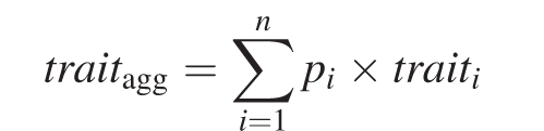where p_i is the relative contribution of species i to the community, and trait_i is the trait value of species i. For categorical traits, the relative contribution of each particular attribute was calculated as the sum of relative abundances of species within that attribute. In both cases, this was calculated with species that collectively make up at least 80 % of the maximum standing biomass of the community.

Ecosystem properties

The ecosystem properties selected for study (Table 2) are key components of the carbon and nitrogen cycles (Chapin et al., 2002). These are: minimum and maximum live standing and dead biomass (terminology after Scurlock et al., 2002), above-ground net primary productivity and specific above-ground net primary productivity (SANPP), rate of litter decomposition, measured both in the field and in microcosms under controlled conditions in the laboratory, or assessed by near infra-red spectrometry.

Net primary productivity (NPP) represents the major input of carbon and energy into ecosystems. It can be considered as an integrative variable of the functioning of the whole ecosystem, owing to its relationships with animal biomass, secondary productivity and nutrient cycling (McNaughton et al., 1989). Although unbiased estimates of NPP are extremely difficult to obtain (Roberts et al., 1993; Scurlock et al., 2002), simple methods may provide fairly good indicators of the general ranking of study sites by productivity (Scurlock et al., 2002). Among those, we chose that based on the difference between maximum and minimum live above-ground biomass (ANPP) for two reasons: (1) it is by far the most frequently reported productivity data in the literature (cf. Esser et al., 2000), allowing us to compare our own data on a very broad scale, and (2) the determination of biomass at two different times allows the computation of SANPP, which expresses productivity on a community biomass basis instead of a ground area basis (see Appendix 2). It was also important to separate live and dead biomass, so as to take into account the specific effects of dead material, as reported in the results section.

In order to separate litter quality effects from impacts on the decomposition environment and decomposer organisms, and hence to refine our understanding of trait-decomposition links, we adopted a three-stage approach (Appendix 2). First, whole community, above-ground vascular plant litter from selected plots at all sites was decomposed in microcosms under standard conditions. Second, a standard litter was decomposed in each plot. Finally, community litter was decomposed in situ, to integrate the combined role of the environment, soil organisms and litter quality.

Standardized protocols for these different measurements were developed. The methods used represent a trade-off between feasibility and biological meaning. Summaries and relevant abbreviations used in the following text are given in Appendix 2, and full documents are available upon request.

Database

A database was designed to standardize the information described above: climate, site characteristics (soil properties, location, altitude, etc.), botanical and ecological information on species, traits, community composition and ecosystem properties. In addition to the general characteristics for the 11 sites, the database currently contains botanical and ecological data for more than 900 taxa, amounting to more than 1000 values for each trait.

Data analyses

Climate

In order to characterize better the climate of the sites a principal components analysis (PCA) was used to investigate the relationships between the sites in terms of mean annual rainfall, mean annual temperature, mean annual PET, annual growing degree-days, mean annual solar radiation and Thornwaite's aridity index. Annual PET and solar radiation were removed after a covariance analysis indicated that they were highly correlated with, in particular, mean annual temperature. Linear projections of the PCA axes were also used as a synthetic climate variable.

Botanical composition

It was not possible to compare the botanical composition of the plots at the species level owing to insufficient overlap in species composition between sites. Instead it was compared at the family level, representing gross scale variation in biogeographical and environmental differences between sites and plots. The comparison was carried out using detrended correspondence analysis (DCA: Hill and Gauch, 1980) using CANOCO v.4 (ter Braak and Šmilauer, 1998) on the percentage contribution of each family to the total cover of higher plants.

Aggregated traits and ecosystem properties

The overall effects of land-use regime within sites on the ten continuous measured traits will be presented here (Table 4). One-way ANOVAs were used to test for differences in aggregated trait values and ecosystem properties across land-use treatments within sites.

Table 4.

Summary of significant differences and direction of response in aggregated means of the ten measured continuous plant traits among treatments (summarized in column 2) in the 11 sites of the VISTA project (results of within-sites one-way ANOVAs)

Site	Disturbance/resource treatments	VPH	RPH	Flower	Seed mass	SLA	LDMC	LNC	LCC	LPC	StDMC	% Traits significant
IS-KDE	Grazing/abandonment	nd	***	ns	ns	ns	ns	*	*	ns	nd	38 (8)
			+					+	+
PT-MER	Agriculture/grazing/abandonment	***	nd	***	*	***	***	ns	***	***	nd	88 (8)
		+		–	+	–	+		+	–
GR-LAG	Grazing/abandonment	ns	**	***	ns	**	ns	*	ns	***	*	60 (10)
			+/–	+/–		–		–		–	–/+
FR-HGM	Abandonment	ns	***	**	ns	***	**	***	ns	*	***	70 (10)
			+	+		–	+	–		–	+
GE-MNP	Grazing/abandonment/water	**	***	***	**	***	***	***	***	nd	**	100 (9)
		+	+	+	–	–	–	–	+		+
CZ-OHR	Mowing/fertilization	***	***	*	*	***	*	*	ns	***	ns	80 (10)
		+	+	+	+	–	+	–		–
SE-BAL	Grazing/abandonment	*	**	*	ns	ns	**	*	ns	nd	**	67 (9)
		+	+	–			+	–			+
SC-SUT	Agriculture/abandonment	ns	nd	***	ns	ns	ns	ns	**	***	**	44 (9)
				+					+	+	+
FR-ERC	Mowing/grazing/fertilization	**	nd	**	*	*	ns	ns	ns	*	*	66 (9)
		–		+	+	–				–	+
FR-LAU	Mowing/grazing/fertilization	***	**	a	ns	***	***	***	ns	**	***	80 (10)
		+	+	+		–	+	–		–	+
NO-BER	Grazing	ns	ns	ns	ns	ns	ns	ns	ns	ns	nd	0 (9)
% Sites significant		60 (10)	88 (8)	82 (11)	37 (11)	64 (11)	55 (11)	64 (11)	36 (11)	78 (9)	88 (8)
Across-sites	Most used/least used	***	***	***	ns	***	**	***	***	***	***	90 (10)
		+	+	+		–	+	–	+	–	+

The last column gives the percentage of traits showing significant differences among treatments within a site (the number in parentheses is the number of traits available at that site), and the penultimate row gives the percentage of sites in which a particular trait varies significantly among treatments (the number in parentheses is the number of sites for which the trait is available). The final row gives the results of a REML analysis contrasting the most and least used treatments across the 11 sites.

Abbreviations: VPH, vegetative plant height; RPH, reproductive plant height; Flower, time of flowering; SLA, specific leaf area; LDMC, leaf dry matter content; LNC, leaf nitrogen concentration; LCC, leaf carbon concentration; LPC, leaf phosphorus concentration; StDMC, stem dry matter content. ns, not significant; a, P < 0·10; *, P < 0·05; **, P < 0·01; ***, P < 0·001. nd, no data. +, increase; −, decrease in response to decreasing land use. Hump-shaped responses are indicated by +/– or –/+.

Inter-site analyses of variation of traits (here LDMC treated as an example) and ecosystem properties (here AGTotDead treated as an example), as well as their patterns of co-variation were tested using restricted maximum likelihood methods (REML) with the statistical package GenStat^® 8·1 (GenStat, 2005). In these analyses, site was used as a random term, and we tested effects of land use, climate (represented by simple variables or the first axis of the PCA on climatic variables) and their interactions, taken as fixed additive terms. In order to test for the effects of community-level traits (here LDMC) on ecosystem properties (here AGTotDead) the same approach was applied, using traits and their interactions with land use as fixed terms in the model.

In the results presented here we compare only the least and most intensively used treatments at each site, while keeping levels as comparable as possible across sites. ‘Most used’ was taken to correspond to ‘traditional use’, usually associated with medium fertility and high biomass removal. ‘Least used’ corresponded to abandonment of these practices. For sites where abandonment was complete, we chose to focus on comparable lengths of succession, using plots with intermediate duration of abandonment (>10 years) vs. recently abandoned sites. At all sites these plots still had a strong herbaceous component.

SELECTED RESULTS

Climatic variables

The 11 sites encompass a large amount of climatic variation. Not only do they differ in terms of total rainfall, temperature (both given in Table 1), solar radiation, etc., but they also vary considerably in the seasonality and periodicity of these climatic parameters. The first axis of the PCA on site climatic parameters (75·7 % of the variation) was largely associated with a gradient of aridity coupled with site temperature and growing degree-days (Fig. 1). PCA axis 2 (22·1 % of the variation) was overwhelmingly linked to annual rainfall, separating two patterns underlying low aridity: high rainfall and moderate temperatures year-round, as opposed to true mountain sites with modest rainfall but low evaporation due to low temperatures during rainy periods. The projections of the sites on the two axes make it possible to separate the following groups of sites: (1) a group of Mediterranean sites with high temperatures and aridity (GR-LAG, PT-MER and IS-KDE: site abbreviations given in Table 1) – FR-HGM is linked with this group by high mean annual temperature but is distinguished by higher rainfall and lower aridity; (2) a group of colder sites but still with relatively low rainfall and medium values of aridity index (GE-MNP, CZ-OHR, SE-BAL); (3) a group of sites with similar temperatures to the above, but characterized by high rainfall and thus low aridity (SC-SUT, FR-ERC); and (4) a group of true mountain sites (FR-LAU, NO-BER) characterized by low temperatures, a short growing season, low aridity and medium rainfall.

Fig. 1.

Principal component analysis on climatic data: mean annual rainfall (Rainfall), mean annual temperature (Temp), annual growing degree-days (GDD, and an aridity index for each site. Annual PET and solar radiation were removed after a covariance analysis indicated they were highly correlated with, in particular, mean annual temperature.

Based on these results we chose to use synthetic climate indices such as the aridity index and projections of sites on PCA axis 1 (Fig. 1) as covariates for analyses of response of traits and ecosystem properties to land use.

Disturbance indices

Disturbance indices of VISTA treatments reflect the wide variety of land-use systems that characterize marginal landscapes across Europe, as shown by the return interval and intensity of disturbances for the least and most used treatments in each site (Fig. 2). The site with the highest disturbance was a short-rotational crop/fallow field in Scotland (SC-SUT: short return interval with the highest intensity), and the lowest was a pasture in Sweden (SE-BAL: longest return interval without disturbance) abandoned for more than 60 years. Aggregated return time of disturbances (Fig. 2A) and biomass removal by disturbance (Fig. 2B) show that the GE-MNP, IS-KDE, PT-MER and SE-BAL sites all span a considerably large range on the disturbance gradient, because they cover situations from continuing, moderately intense management to advanced secondary succession. The magnitude in disturbance regimes is more restricted at the NO-BER, FR-ERC, FR-LAU and FR-HGM sites. Among these, FR-ERC treatments are highly disturbed, whereas the abandonment sequence at FR-HGM belongs to the lower end of the total VISTA disturbance gradient. All other sites are intermediate with respect to variation in either disturbance frequency or biomass loss.

Fig. 2.

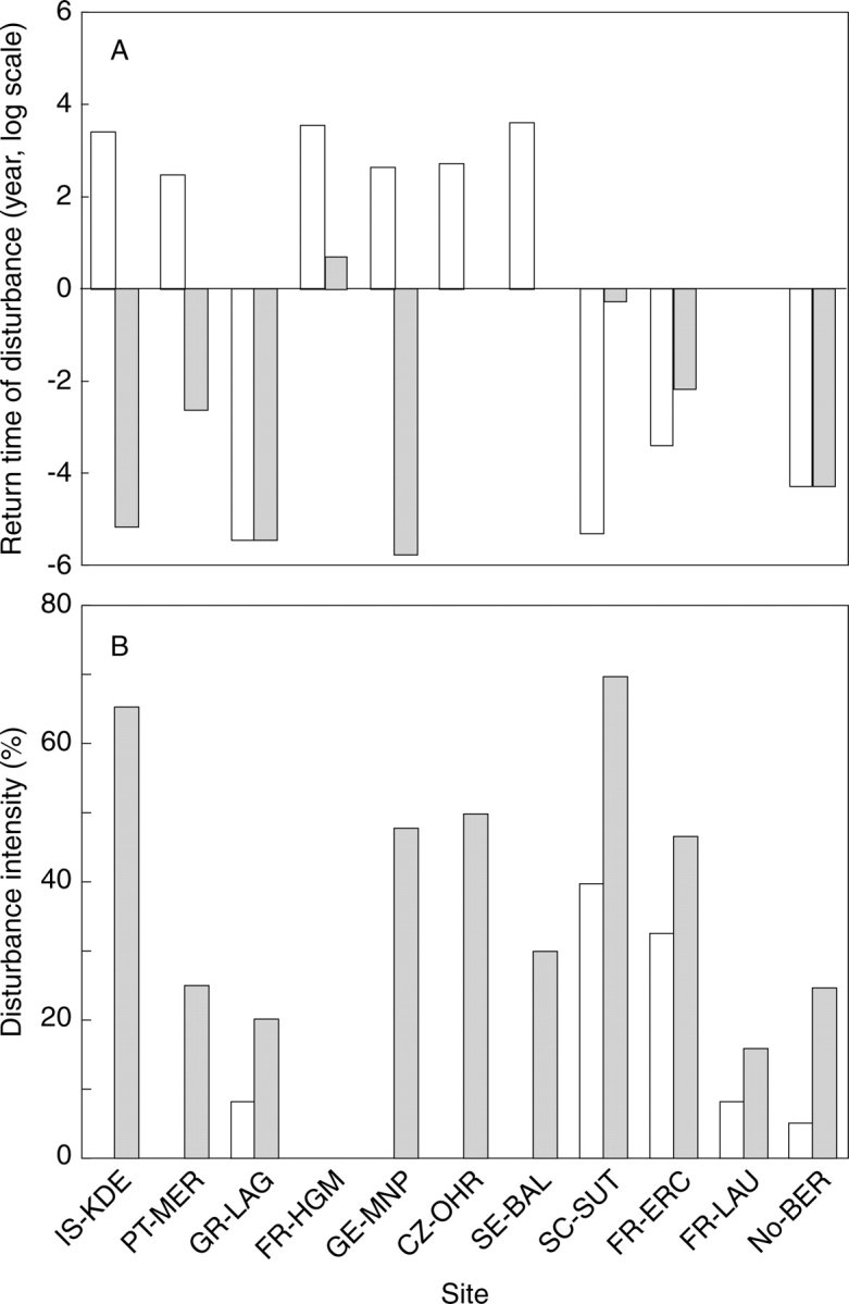
(A) Return interval (log scale) and (B) intensity (expressed as a percentage of maximum standing biomass) of disturbance for the least (open columns) and most (shaded columns) intensively used treatments in each site. In A, a value of 0 indicates a return interval of 1 year (e.g. both treatments in FR-LAU), whereas in B a value of 0 corresponds to a lack of biomass removal (e.g. both treatments in FR-HGM).

Vegetation

The DCA (Fig. 3) revealed significant turnover at the family level across all the sites and plots for the first two axes of the ordination (axes lengths of 6·58, 5·88, 2·82 and 2·55, respectively). These first two axes also explained a substantial part of the variation (percentage of total inertia explained of 10·9 and 8·1 compared with 3·5 and 2·8 for axes 3 and 4, respectively). The ordination clearly showed that many of the sites were relatively similar in cover at the family level with a dominance of Poaceae, as well as Apiaceae, Asteraceae, Rosaceae, Caryophyllaceae and Plantaginaceae. At high values on Axis 1 were the Norwegian sites (NO-BER) characterized by substantial cover of Ericaceae and Salicaeae, as well as the late successional Swedish sites with high values for the Ericaceae. Low values on Axis 1 were associated with Mediterranean woodland and scrub-dominated plots, including the GR-LAG and PT-MER sites dominated by Cistaceae and Fagaceae (Axis 1 scores of approx. 3).

Fig. 3.

Detrended correspondence analysis (DCA) of relative abundance of higher plant families for each recorded plot. Only families with a weight of >2 % of the maximum family's weight are shown as the first eight letters of their full name.

Responses of plant traits to land-use change: an overview

Continuous traits (aggregated values) can be grouped into three categories, according to their sensitivity to treatments across sites (Table 4): (1) traits that respond to treatments in most sites – reproductive plant height, stem dry matter content, leaf phosphorus concentration and flowering time; (2) traits that respond in half to two-thirds of the sites – specific leaf area, vegetative plant height, leaf nitrogen concentration and leaf dry matter content; and (3) traits that respond in approx. one-third of the sites – seed mass and leaf carbon concentration. The REML analysis across the 11 sites highlighted strong and consistent responses across sites for all traits except seed mass. Direction of change was overall consistent for all traits with a significant response. Decreasing land use resulted at the community level in dominance by taller plants (increased vegetative and reproductive height), plants with more conservative leaf syndromes (decreased SLA, LNC and LPC, increased LDMC associated with increased StDMC), and delayed flowering phenology. These responses were overall strongly consistent across sites, and the few exceptions resulted from either canopy closure after woody colonization (e.g. Sweden, Greece) or specific soil conditions (water-logging in Germany).

Multivariate analyses conducted at four individual sites identified consistent patterns in variation in plant strategies. At the SC-SUT site, Pakeman and Small (2004) showed that land use was a significant predictor of plant traits as abandonment of rotational cultivation led to an increase in species with more conservative nutrient use, had later flowering and larger seed sizes. However, species composition did not recover in the direction expected from analysis of unploughed areas. Overall, these results were repeated at the French alpine site (FR-LAU), where cessation of fertilization or of mowing resulted in the dominance by taller plants with more conservative nutrient use and later flowering, although seed mass did not vary across land-use treatments (Quétier et al., 2006). A path analysis conducted on the data from the French Mediterranean site (FR-HGM) demonstrated that abandonment of vine cultivation led to the progressive replacement of species with small stature, high rates of resource capture and early flowering by species with the opposite characteristics, while seed mass did not show any significant trend with time after abandonment (Vile et al., 2006). Finally, Lepš (1999) demonstrated significant changes in species composition as a response both to fertilization and to cessation of mowing. Plant height was a very good predictor of species success under fertilization, as only tall plants were able to survive in competition.

Responses of ecosystem and soil properties to land-use change: an overview (Table 5)

Table 5.

Summary of significant differences and direction of response to decreasing land use in selected ecosystem, community and soil properties among treatments (summarized in column 2) in the 11 sites of the VISTA project (results of within-sites one-way ANOVAs)

Site	Disturbance/resource treatments	AGBmass	AGTotdead	ANPP	Knat-lab (NIRS)	Soil C	Soil N	Soil P-Olsen	NNI	PNI	Species richness	% Properties significant
IS-KDE	Grazing/abandonment	***	***	***	***	ns	ns	*	*	**	***	80 (10)
		+	+	+	–			+	–	+	–
PT-MER	Agriculture/grazing/abandonment	**	*	*	**	*	a	***	ns	**	**	90 (10)
		+	+	–	–	+		–		–	–
GR-LAG	Grazing/abandonment	***	***	***	ns	***	***	**	*	***	***	90 (10)
		–	–/+	–		+	+	–/+	+/–	–/+	+/–
FR-HGM	Abandonment	*	*	*	a	***	***	ns	ns	ns	**	70 (10)
		+	+	–	–	+	+				–
GE-MNP	Grazing/abandonment/water	***	***	***	*	a	***	***	nd	nd	***	100 (8)
		–	–	–	–	–	–	+			–
CZ-OHR	Mowing/fertilization	ns	***	ns	**	ns	ns	***	a	***	***	60 (10)
			+		–				–		–
SE-BAL	Grazing/abandonment	**	**	**	***	***	**	a	ns	nd	*	89 (9)
		–	+	–	–	+	–				–
SC-SUT	Agriculture/abandonment	ns	ns	ns	ns	ns	*	*	ns	*	*	40 (10)
							+	–		–	+
FR-ERC	Mowing/grazing/fertilization	a	ns	*	ns	ns	ns	*	*	**	**	60 (10)
		–		–				–	–	–	+
FR-LAU	Mowing/grazing/fertilization	ns	*	ns	***	ns	ns	*	a	ns	*	50 (10)
			+		–			–	–	–	–
NO-BER	Grazing	nd	nd	nd	ns	ns	ns	ns	nd	nd	a	20 (5)
											+
% Sites significant		70 (10)	80 (10)	70 (10)	64 (11)	55 (11)	64 (11)	81 (11)	56 (9)	75 (8)	100 (11)

The last column gives the percentage of ecosystem/soil properties showing significant differences among treatments within a site (the number in parentheses is the number of ecosystem/soil properties available at that site), and the last row gives the percentage of sites in which a particular property varies significantly among treatments (the number in parentheses is the number of sites for which the property is available).

Abbreviations: AGBmass, maximum live standing biomass; AGTotdead, total dead material (standing dead+litter) at peak standing biomass; ANPP, above-ground net primary productivity; K_nat-lab (NIRS), decay rate assessed by near-infrared spectrometry; Soil C and N are total soil carbon and nitrogen concentrations, respectively; Soil P-Olsen is plant-available phosphorus; NNI and PNI are the nitrogen and phosphorus nutrition indices, respectively. Species richness is the number of species recorded in each plot. ns, not significant; a, P < 0·10; *, P < 0·05; **, P < 0·01; ***, P < 0·001. nd, no data. +, increase; –, decrease in response to decreasing land use. Hump-shaped responses are indicated by +/– or –/+.

Maximum above-ground live (AGBmass) and dead biomass (AGTotDead) were significantly different among treatments in ten out of the 11 sites, but the effects of treatments were not necessarily comparable for the two variables (Table 5). By contrast, owing to the very tight correlation between maximum AGBmass and ANPP within (data not shown) and across sites (r = 0·89, P < 0·001, n = 170), the effects of treatments on these two variables were identical. Treatments had significant effects on average community decomposition rate measured under standard conditions, when there was no interaction with environmental conditions, in six out of the 11 sites. This reflects a decline in litter quality (C. Fortunel et al., unpubl. res.), which is a major determinant of in situ decomposition rates (Swift et al., 1979; Lavelle, 1993). The results of the in situ experiment are more complex (data not shown), however, as changes in the decomposition environment within sites also play a major role.

There was also a very close relationship between soil C and N both within (not shown) and across (r = 0·87, P < 0·001, n = 194) sites, with the consequence that treatment effects were almost identical on the two variables (the SC-SUT site being the only exception). Interestingly, nitrogen limitation as detected by the NNI had little concordance with information given by soil N. Phosphorus availability to plants as detected by soil P-Olsen was significantly different among treatments in nine of the sites, and except for two sites (IS-KDE and FR-LAU), these differences were consistent with those found using the PNI.

A methodology to link changes in disturbance regime, plant traits and ecosystem properties

One of the methodologies that can be used to assess the effects of land-use change on the functional properties of the vegetation through plant traits and environmental variables consists in successive sets of general modelling analyses. We present here the case of leaf dry matter content and above-ground total dead biomass as an illustration. The approach consisted of first identifying the effects of climate and land-use factors on LDMC, and then testing whether land-use effects on AGTotdead may be explained by changes in LDMC and/or in climate.

Accumulation of dead material represents the net balance between rates of production and decomposition of dead matter. Decomposition has been shown to be slower in litter produced by plants with high leaf dry matter content (Garnier et al., 2004; Kazakou et al., 2006). Our hypothesis was therefore that a reduction of management pressure would cause litter to accumulate in communities as LDMC increased due to slower decomposition (Tables 4 and 5). We further investigated whether interactions with climate were detectable across sites.

Figure 4A shows that across sites, less intensive land use led to communities with higher LDMC-aggregated values (Wald statistic = 8·45, P < 0·001). Within sites, differences were significant for five sites, but the direction of change was consistent for ten of the 11 sites. Aggregated LDMC tended to decrease with mean annual temperature (P = 0·10) but not with aridity or the first axis of the PCA. The increase in LDMC in response to less intensive land use was greatest at warmest sites (significant interaction; Wald statistic = 21·73, P < 0·001), possibly as a result of a higher intensity of land use increasing the dominance by annuals at the warmest (and especially Mediterranean) sites. At sites where the differences in LDMC among treatments were largest, dead material tended to accumulate in large quantities (Fig. 4B). The quantity of dead biomass was, in some plots, up to four or five times greater than the live standing biomass, with the largest differences evident in abandoned plots (e.g. FR-HGM, CZ-OHR, SE-BAL). As hypothesized, there was a positive relationship between aggregated-LDMC and above-ground dead biomass (Fig. 5). Five points appear as outliers in this relationship: three are from the CZ-OHR site (open circles) and two from the FR-HGM site (closed squares). In these two cases, the plots concerned are dominated by large tussock grasses with high LDMC leaves (Molinia caerulea in the Czech site, Brachypodium phoenicoides in the French site). The large accumulation of dead biomass in these plots is probably linked to the combination of high biomass production, substantial leaf turnover and particularly low rate of decomposition of the litter produced by these species. For example, we have shown that the rate of decomposition of the litter produced by B. phoenicoides was the lowest among the species screened at the Mediterranean site (Kazakou et al., 2006).

Fig. 4.

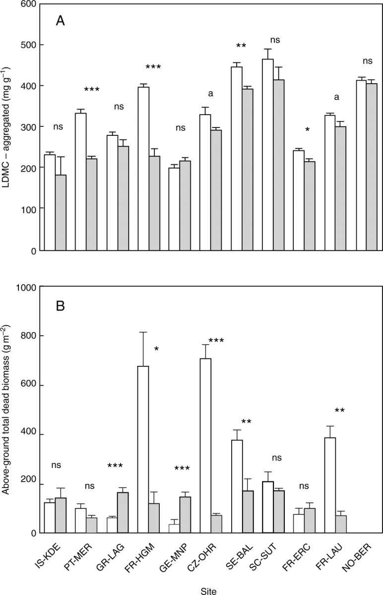
(A) Community-aggregated values of leaf dry matter content (LDMC), and (B) above-ground total dead material (which includes standing dead biomass and litter fallen on the ground) at the time of peak biomass for the least (open columns) and most (shaded columns) intensively used treatments in each site. Significance of tests by one-way ANOVAs within sites is indicated: ns: not significant, P>0·10; a, P < 0·10; *, P < 0·05; **, P < 0·01; ***, P < 0·001.

Fig. 5.

Relationship between community-aggregated leaf dry matter content (LDMC) and above-ground dead biomass (AGTotdead) at the time of maximum standing biomass across ten sites of the VISTA project, using the least/most used treatments in each site. r values are Pearson correlation coefficients for all data (top value) and when the five points with AGTotdead values higher than 600 g m⁻² were removed (in parentheses); n is the number of data points (***, both relationships are significant at P < 0·001).

Across sites, both land use and LDMC significantly influenced total dead biomass (Wald statistics = 33·61 and 36·29, respectively, P < 0·001 in both cases). In the ‘most used’ plots, total dead biomass was significantly lower than in less disturbed plots, and plots with increasing LDMC had greater total dead biomass. A significant interaction term (P = 0·007) indicates that the higher the mean LDMC at a site, the greater the effect of utilization in reducing the amount of dead matter. However, no significant effects of mean annual temperature or any other climatic variables on total dead biomass were detected.

Together, these results suggest that owing to higher litter input rates, and/or lower decomposition rates, dead matter accumulation is greater in less disturbed conditions. Community aggregated LDMC provides a good indicator of these changes. This relationship emerges partly because both LDMC and litter inputs decline with increasing land use. A further potential mechanism is that litter produced by plants with a higher LDMC decomposes more slowly (Garnier et al., 2004; Kazakou et al., 2006), leading to a longer residence time for such litter in the plots. Furthermore, it is interesting to note that, across sites, the correlation between above-ground total dead biomass and LDMC is significant for least used plots (r = 0·86, P < 0·001) but not for most used plots. This is in part explained by the much lower range of variation in LDMC across most used plots.

DISCUSSION

A plea for standardized protocols

Considerable efforts to standardize the measurements of plant traits have been developed in recent years (Hendry and Grime, 1993; McIntyre et al., 1999; Cornelissen et al., 2003; Knevel et al., 2005). This has resulted in a rapidly increasing global coverage of data sets on plant traits (Niinemets, 2001; Reich and Oleksyn, 2004; Wright et al., 2004; Díaz et al., 2004; Moles et al., 2005), which become available in easy and normalized format following the development of trait databases (Grime et al., 1988; Fitter and Peat, 1994; Knevel et al., 2003; Wright et al., 2004). This collective, worldwide effort is a cornerstone in the development of a more consistent view of how the environment shapes the design and functioning of plants (e.g. Grime, 2001; Westoby et al., 2002).

This is only one part of the story, however. If we are to understand quantitative relationships between plant functioning and (1) environmental factors on the one hand, and (2) ecosystem functioning on the other hand, standardization for other variables is necessary. The first issue, which constitutes one of the four themes for ‘a functional trait research program’ as proposed by McGill et al. (2006), requires a careful quantification of environmental gradients. Even if, say, a trait is theoretically responsive to a particular gradient, the detection of this response will depend on the range of variation in the environmental factors underlying this gradient (Wright et al., 2005). This is one of the key reasons why these need to be quantified with objective, comparable variables and methodologies. To address the second issue, it is necessary to select which ecosystem properties are the target of study, and to use normalized protocols for their measurements.

In the following we discuss the lessons learned through our test at the 11 VISTA sites on four main topics of broad interest to future research: the quantification of environmental gradients, the relevance of the traits selected for study and of trait aggregation, how community traits contribute to ecosystem properties, and methodologies for advanced data analysis.

Quantification of environmental gradients

In inter-site analyses of trait and ecosystem property responses to land-use change, environmental gradients can be grouped into three main categories: climate, disturbance and resource availability.

Climate

Although simple measures of climate (e.g. temperature, rainfall) may sometimes be useful to predict species/trait responses, both often respond to overall climatic conditions (integration of all aspects of climate). In addition, redundancy among variables (e.g. between mean annual temperature and solar radiation) should be avoided as much as possible when applying traditional statistical methods such as general modelling or multivariate statistics. These problems can be solved by using synthetic indices such as Thornwaite's aridity index, simple indices of rainfall effectiveness (rainfall compared with PET), or linear projections of climatic variables on the PCA axes in Fig. 1. Calculations of these indices limited to the actual growing season at each site may better capture this ‘integrated’ aspect of the climates at the different VISTA sites. Inter-site analyses such as those presented here for leaf dry matter content (LDMC) and above-ground total dead biomass (AGTotDead) illustrate this by including climatic variables as covariates. Alternative approaches could also be developed by applying structural equation modelling (SEM) to identify direct and indirect effects of the full set of climate and other environmental variables on plant traits and ecosystem processes (see Vile et al., 2006).

Disturbances

Across sites, the range of disturbances encompassed in the VISTA project corresponded to the wide variety of land-use transitions currently occurring in marginal agricultural situations in Europe. Within sites, differences in disturbance regimes are large when agricultural use (grazing, mowing, crop cultivation) is compared with long-term abandonment. Differences are small when either agricultural land uses of different intensity or different stages of abandonment are compared. Our assumption is that there are general commonalities of the effects of disturbance regime on plants regardless of the disturbance type (mowing, ploughing, etc). These effects operate through the intensity (the amount of biomass loss), the return interval (time for biomass recovery) and the onset (the phenological stage affected by a disturbance impact) of disturbances, while pretreatment regimes and type of disturbances (identity of grazers in particular), which are categorical variables, operate as co-variates. Characterization of disturbance regimes by such descriptors was proposed by White and Pickett (1985) and White and Jentsch (2001). In principle, they are designed to parameterize the effects of any disturbance, either natural hazards (e.g. flooding, fire) or human land use. In practice, however, this task is not yet sufficiently solved. Although intensity of biomass loss could be adequately assessed, e.g. by using exclosures in the case of grazing, the parameterization of return interval still represents a problem. A relatively short period of grazing, e.g. 10 days per year, results in a higher return interval than five mowing events per year. This is unsatisfactory because the different spatial scales of the two disturbances regimes are not taken into account. Land uses comprising a rotation of fallow and cultivation periods (PT-MER, SC-SUT) are also insufficiently characterized by a single figure for return interval and intensity of biomass loss.

Regardless, whether disturbance stands out as a relevant predictor of plant traits and ecosystem properties may critically depend on the variation of disturbance compared with the variation of other factors such as fertility or water availability. In addition, the impact of disturbances is context-dependent across gradients of resource availability, particularly those limiting productivity.

Soil properties and nutrient availability

Although standard methods to determine soil variables are available, these are not unique, and the panel of variables is large (cf. Page, 1982; Sparks, 1996). The variables available for standardized, relatively easy measurements in the field are also only proxies for ‘latent’ variables that are hypothesized to determine ecosystem dynamics (see Weiher et al., 2004), just as ‘soft’ traits are used to access ‘hard’ traits (Hodgson et al., 1999). Beyond soil standard properties such as pH and texture (from which water-holding capacity of plots was derived), the soil data collected relate to pools rather than availability of nutrients (but see below for phosphorus). Concerning C and N, routine procedures allow the determination of total contents, which are directly related to total organic matter content. There is currently no simple method to assess the amount of nitrogen a given soil can release and make available to plants. Existing methods (Bundy and Meisinger, 1994) are time consuming and difficult to run in series (soil incubations), making the assessment of nitrogen availability for a large number of samples problematic. Therefore, and because total soil N content is not informative of N availability, NNIs have been developed (Lemaire, 1997). NNI is based on plant N concentration determination and directly provides the vegetation nutrient status in relation to the degree of growth. The NNI has been successfully applied to diagnose N nutritional status on mixed crops (Cruz and Soussana, 1997) as well as native grassland (Duru et al., 1997). When applied to the VISTA experimental sites, there was a higher correlation between ANPP and NNI across sites (r = 0·79, P < 0·001, n = 94) than between ANPP and total soil N (r = 0·64, P < 0·001, n = 94), and NNI explained a greater part of the variance than any of the climatic indices.

As for phosphorus, although total soil P content does not give the amount of available P released from soil, several P availability indices can be obtained routinely (Kuo, 1996). Among those, Olsen P (Olsen et al., 1954) has been chosen here, as the method gives better characterization than other chemical extraction over a large range of pH, from calcareous to slightly acidic soils (Morel et al., 2000). It is also widely used for all soils types in a large number of countries (Sibbesen and Sharpley, 1997). To complement these data, we also calculated a PNI, based on simultaneous measurements of N and P concentrations of the vegetation (Appendix 1). PNI, which has been developed to assess the phosphorus nutrition status in grasslands, was positively correlated with Olsen P values within sites (data not shown) as already found by Jouany et al. (2002). However, no relation exists between these two variables at the inter-site level.

The trait toolkit and some consequences of the aggregation procedure

The trait toolkit

The trait list we used was derived from that proposed by Weiher et al. (1999), initially designed as a toolkit to predict vegetation responses to disturbances at the species level. It was used here at the community level, through the calculation of community-aggregated traits. One of the premises of functional plant ecology is that plant traits can be used as a general tool to analyse plant–environment relationships across biomes. From Norway to Portugal, the botanical composition (Fig. 3) is indeed very different. Which of the traits actually appeared as response traits to land-use changes across the VISTA sites?

Our results suggest that reproductive plant height responds more consistently than vegetative plant height (VPH) to land-use change (Table 4). Three reasons related to the fact that data have been collected mainly on herbaceous species may explain this result. First, it is sometimes difficult to define VPH from a morphological perspective. For example, some annual grasses produce only one rapidly heading tiller, and in some dicots a flowering stem is produced without a clearly marked vegetative stage. Second, in herbaceous plants, VPH may be highly dynamic over the growing season, as it follows vegetative growth, at least to a certain extent. This has two consequences: (1) it is highly sensitive to the date of data collection, and (2) it is very variable among replicate plants, as individuals of the same population may not necessarily be at the same developmental stage at a fixed sampling date. And third, for rosette and prostrate species, plant stature bears no particular relationship to VPH. If the objective is to assess the general stature of a plant and growth is not the target of the study, we therefore suggest that reproductive plant height (RPH), which does not suffer from the same experimental and ontogenetic problems as VPH, be used rather than vegetative height. In herbaceous species, RPH should thus be added to VPH in the trait lists proposed for functional ecology (Weiher et al., 1999; Westoby et al., 2002).

Our data also confirm that leaf traits involved in the acquisition–conservation trade-off (Chapin et al., 1993; Grime, 2001; Wright et al., 2004) such as SLA, LDMC, LNC and LPC are key to the analysis of functional responses to changes in land-use intensity (Table 4): a reduction of the grazing pressure and/or fertility and an abandonment of land tend to favour species with reduced acquisition capacities and increased nutrient conservation efficiency. Stem dry matter content can be linked to this group of traits, and appears to be quite responsive as well. However, this trait is not always easy to measure, in particular because it is not easy to assess whether rehydration of the stem prior to measurement is complete. Even though StDMC – a proxy of stem tissue density – plays an important role for the structure and functioning of woody species (see Cornelissen et al. 2003, and references therein), we suggest that its efficacy and standardized measurement have not been sufficiently established to recommend its standard use in studies involving mainly herbaceous species.

Onset of flowering (OFL) was one of the traits most sensitive to land-use changes (Table 4), although this trait is not commonly documented, e.g. in grazing studies (see Díaz et al., 2006). Reduced grazing, lower fertility and land abandonment promoted delayed flowering, consistent with the idea that early flowering reflects disturbance avoidance (Weiher et al., 1999; Pakeman, 2004). More generally, these variations in OFL can be interpreted as a change from ruderal to competitive strategies (cf. Grime, 2001; Kahmen and Poschold, 2004; Pakeman, 2004), in line with the fact that large plants tend to flower late. By contrast, seed mass, a trait that authors tend to focus on more frequently, was responsive to treatments in less than half of the sites (Table 4). This does not support the theoretical expectation that small seeded species, with increased probabilities of dispersal, should be favoured in disturbed habitats (Grime, 2001; Weiher et al., 1999, and references therein). It may be explained by the fact that seed mass varied by up to five orders of magnitude within individual treatments, so that any patterns of response were obscured by natural variance.

Against these general trends, trait responses were variable across sites and need to be related to the ranges of within-site variations of (1) disturbances and fertility (see above), and (2) inter- vs. intra-treatment variability in trait values.

Further differences across sites in trait responses will be analysed using climate variables as covariates, as done here for the LDMC example (see also Díaz et al., 2006). Analyses would also need to include the contribution of changes in life-form frequency as a covariate (cf. McIntyre et al., 1999), for example changes in grasses vs. forbs, and increases in the representation of annuals in more disturbed treatments.

Apart from the restrictions discussed above, our trait list finally appears to capture adequately the functional response of herbaceous-dominated vegetation to land-use changes, even though they differ in nature and intensity across sites. Although we expect the core of the trait list to be generic, it would need to be refined for application to woody vegetation, as relevant traits to response to land use and other disturbances can be life-form specific (McIntyre et al., 1999).

On the use of community-aggregated plant traits

Community-aggregated traits were used here to detect the average functional response of vegetation on the one hand, and to relate this response to ecosystem functioning, as a test of the biomass ratio hypothesis (Grime, 1998). When the aggregated traits are calculated for variable traits, i.e. for traits differing in value according to treatment levels, then a change in their values can be caused either by variability of traits within species (e.g. a species has lower LDMC in nutrient-rich moist treatment than in nutrient-poor dry treatment), or by a change in species composition (in a nutrient-rich moist site, species composition is shifted toward a higher proportion of species with inherent low LDMC). For the test of the mass ratio hypothesis of ecosystem functioning, the change in aggregated traits is probably the most important community characteristic, regardless of whether the change was achieved through variability within species or through change in species composition. For many conservation and biodiversity studies, however, it is extremely important to know to what extent is this change caused by change in species composition. In this case, we can reverse the question, asking ‘which traits cause the species to be responsive to environmental change’ (e.g. de Bello et al., 2005). Methods are being developed to separate the effect of species composition change from the effect of trait variability within species. Species-level analysis, in contrast to community-level analyses such as those presented here, would also need to account for possible phylogenetic effects.

Components of ecosystem functioning

Our research has focused on the links between species traits and biogeochemistry, with the central hypothesis that traits involved in fundamental trade-offs such as the acquisition/conservation trade-off discussed above would scale up to components of carbon and nutrient cycles at the ecosystem level (Chapin, 1993; Lavorel and Garnier, 2002). The two ecosystem processes selected (NPP and litter decomposability) are key components in these cycles (Chapin et al., 2002). NPP represents the major input of carbon into ecosystems, and it also integrates across the system in depending on climate, nutrient supply, removal by animals, as well as the traits of the plants present.

The fate of NPP is important. Accumulation of dead material has important implications for productivity and community composition (Grime, 2001; Facelli and Pickett, 1991), plays a role in regulating soil moisture (Heady, 1956), and can be a major determinant of carbon and nutrient storage and fluxes through ecosystems (Chapin, 1993). The magnitude of the (short-term) effects of dead material on plant communities can be comparable with those of competition or predation (Xiong and Nilsson, 1999), or site fertility (Sydes and Grime, 1981), and litter build-up can have major implications for species conservation (Lennartsson and Svensson, 1996; Eriksson and Ehrlén, 2001). Shifts in land use and plant species composition can influence decomposition by a number of mechanisms, including changes in the quality of the litter produced and influences on the temperature and moisture regime at the soil surface (Eviner, 2004). The proposed three-step methodology, quantifying potential decomposability in vitro, changes in the decomposition environment and their combined effects on decomposability in situ, provides a simple and accessible method for estimating the relative decomposabilities (sensu Cornelissen, 1996) of litter produced at different sites. It thereby enables broad comparisons of changes in the decomposition environment and function of the soil decomposer community in response to land-use change. However, although it is becoming increasingly clear that plant species identity can have marked effects on below-ground processes (Binkley and Giardina, 1998; Eviner, 2004; Reich et al., 2005), the links between litter quality, short-term mass loss of litter and processes such as nutrient cycling and accumulation of soil organic matter are far from clear (Latter et al., 1998; Prescott, 2005). Despite its extremely widespread use as a simple, standardized and easy-to-use tool for comparative decomposition studies, the litterbag method has some drawbacks (see, for example, Heal et al., 1997). Future work needs to be aware of the limitations of focusing on the early stages of decomposition, and to develop simple, standardized measurements of other aspects of soil processes.

Data collected following the approach proposed by VISTA makes it possible to analyse direct effects of climate and land use on ecosystem properties vs. indirect effects via changes in plant traits. Indeed, land use also affects ecosystem properties directly, for example through fertilization, direct biomass removal or physical alteration of soils (e.g. trampling). This approach was illustrated above in the case of LDMC and standing dead biomass (Fig. 6), and discussed in the case of litter decomposability. For instance, our results highlighted that land use may affect standing dead biomass in two ways: (1) directly – increasing land use leads to decreasing litter accumulation, e.g. through biomass export or direct physical effects (e.g. trampling); and (2) indirectly – increasing land use leads to decreased LDMC. Because LDMC is positively correlated with litter accumulation, a negative effect of land use on litter ensues. These relationships are enhanced for sites with higher mean annual temperature both because decreases in LDMC in response to land use are greatest at warmer sites, and because decreases in litter accumulation in response to land use are greatest at warmer sites (Fig. 6). Finally, direct vs. indirect effects of land use may operate through the modification of soil properties, including land-use legacies (Fraterrigo et al., 2006; Quétier et al., 2006). In the same way that experimental approaches have been used to tease out the effects of different components of grazing on vegetation (e.g. Kohler et al., 2004), manipulative experiments that can isolate direct effects of climate and land use from indirect effects via changes in community functional composition are required to advance our understanding of the role of traits as linkages between environmental change and ecosystem properties.

Fig. 6.

Articulating direct and indirect effects of environmental factors and land use on plant traits and ecosystem properties. The relationships are illustrated here based on the results obtained for community-aggregated LDMC and standing litter (AGTotdead). The arrows represent significant statistical relationships, with +/− signs indicating the direction of effects.

Data handling and analyses

The VISTA project has collected and collated a large quantity of data of various types (climate, soil, traits) and scales (species, community, ecosystem). These data have been linked within the database to allow efficient management and flexibility in developing data analysis.

As briefly illustrated in this paper, these analyses can take a number of different forms: multiple measurements per species (as many occur in more than one site and more than one treatment) allow intra-specific variation in traits to be analysed; trait responses can be examined at different scales (within site or across sites) and levels of organization (population or community); trait responses can also be compared for consistency between the site scale and the European scale, and the effects of climate and other abiotic variables on these responses considered; traits can be examined individually (univariate) or in groups (multivariate). For instance, all leaf traits could be examined within the same analysis rather than separately, thus acknowledging that leaf traits co-vary (Díaz et al., 2004; Wright et al., 2004). The large numbers of species should make it possible to investigate phylogenetic correlations and robustly to test trait responses within life forms, as suggested by McIntyre et al. (1999).

The analytical procedures must also be appropriate and informative. They must consider the structure of the data – for example testing across sites needs linear mixed modelling rather than regression. They must also be capable of apportioning variation into different sources – allowing the examination of relationships between traits, land use, soil or climate to be done separately. Multivariate testing allows the simultaneous testing of suites of traits that might co-vary (e.g. leaf traits) or that might show little individual variation but show significant patterns when taken together. Finally, recently developed methods such as SEM will make it possible to test multivariate hypotheses regarding direct and indirect paths of causal linkages with multiple, generalized independent and dependent variables (e.g. Vile et al., 2006).

CONCLUSIONS

We have proposed a methodological framework, along with standardized protocols, to collect and analyse the large data sets that are required to test recent hypotheses regarding linkages between species and ecosystem functioning through plant traits. The application of this methodology for 11 sites representing a large diversity of climatic and land-use conditions across Europe has confirmed the relevance of plant traits associated with the nutrient acquisition–conservation trade-off to understand the response of ecosystems to land-use change. It has highlighted other useful morphological and regeneration traits such as reproductive plant height and flowering phenology. Including environmental variables such as standardized descriptors of climate, soil and disturbance in quantitative analyses makes it possible to test hypotheses about the pathways that ultimately determine ecosystem properties directly, and indirectly through modification of plant trait representation in communities. The proposed framework and methodologies are generally applicable to analyse the impacts of global change drivers on species, communities and ecosystems.

APPENDIX 1

NITROGEN AND PHOSPHORUS NUTRITION INDICES

These indices were determined from above-ground live biomass data and chemical analyses conducted on this harvested biomass. When legume species were present in a sample, they were sorted by hand before chemical analysis, or their contribution to live above-ground biomass (AGBmass) was estimated in order to introduce a correction to the calculated NNI (se below). Nitrogen and phosphorus concentrations were determined from oven-dried (80 °C) ground material (0·5 mm). Total N concentration (%N) was determined either with a CN elemental analyser or with a Kjeldahl protocol following a digestion procedure, while total P (%P) was obtained following wet digestion in H₂SO₄/H₂O₂ using the ceruleomolybdic blue method (Murphy and Riley, 1962). From these measurements, the nitrogen (NNI) and phosphorus (PNI) nutrition indices were calculated (Duru and Ducrocq, 1997; Duru et al., 1997; Lemaire, 1997):

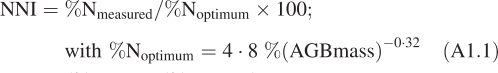A1.1

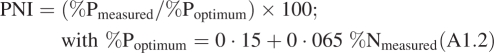A1.2

When %N is determined on biomass including legumes, a correction on the calculation of NNI is required (NNI_c and PNI_c, respectively) in order to avoid overestimations due to the ability of legumes to fix atmospheric nitrogen (Jouany et al., 2005; Cruz et al., 2006):

A1.3

A1.4

APPENDIX 2

METHODS FOR ECOSYSTEM PROPERTIES

Components of primary productivity

At least two harvests of above-ground biomass were conducted in a specific growing season at each site, to assess minimum and maximum standing biomass. This was done for all plots, each plot being considered as a treatment replicate. The details of the protocols differed, depending on type of vegetation and whether the plots were grazed or not. Permanently fenced subplots were usually used in grazed areas. In the small number of plots where woody species were present, harvests were conducted on the herbaceous layer.

An area of approx. 1 m² per plot was sampled, which appears acceptable in this type of vegetation (cf. Wiegert, 1962; Roberts et al., 1993). This area comprised smaller sample units (quadrats or circles) spread over each plot. All above-ground material (live and dead) within sampling units selected on each harvest date was collected by clipping at ground level. On this harvested biomass, live material was separated from the dead. These two fractions were then oven-dried (or freeze-dried) to constant mass at 60 °C and weighed. Above-ground net primary productivity (ANPP) was then calculated (‘Method 3’ of Scurlock et al., 2002):

A2.1

and specific above-ground net primary productivity (SANPP) was calculated (Garnier et al., 2004):

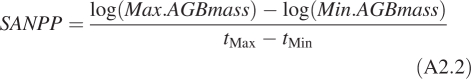A2.2

where Min. and Max. refer to the periods of minimum and maximum above-ground live standing biomass (AGBmass), respectively.

Litter decomposition

Litter collection

At the time of the major peak of natural senescence, litter of all plant parts of all vascular plant species was collected in the proportions in which it is naturally shed in the plots (Hector et al., 2000; Knops et al., 2001). Coarse woody litter (>5 mm diameter), live biomass, substantially decomposed material and seeds were excluded. In sites where there was more than one, or a long, senescence peak, several litter collections were mixed to form one ‘community litter’ (Aerts et al., 2003). Hay was chosen for the standard material. Native and standard litter were cut into 5-cm lengths, so that litter could be contained within the litter bags and each litter bag could contain a representative mixture of different plant parts and species (Dukes and Field, 2000). Litter was dried at room temperature (approx. 20 °C) for 3–4 d.

A standard 1-mm mesh (Northern Mesh, Oldham, UK) was used in all sites. Litter was weighed into 2-g (±0·1 g) portions, and placed into flat litter bags, of approx. 10 × 10 cm. Subsamples (2 g) for air dry weight to oven dry weight conversion were made. A standard procedure was followed for dealing with litter spillage.

Field decomposition

Incubation was initiated as soon as possible after the peak of natural senescence. Community litter was incubated in the plot from which it came. A minimum of seven litter bags per plot, harvest and litter type (community or standard) were placed on the soil surface (minimum 42 bags per plot). Where necessary, small exclosures were used to protect bags from grazing animals, and vice versa. Vegetation in exclosures was clipped regularly during the growing season to match the height of vegetation in the plot as a whole.

Three harvests were made across all sites and plots, after approx. 6, 12 and 18 months. In sites with very rapid or strongly seasonal decomposition patterns, an additional harvest, after 3 months, was performed. Standardized harvesting guidelines were followed by each partner. Any extraneous plant material, large soil animals and soil aggregates were carefully removed by hand. Ashing of litter samples was only carried out at sites where soil ingress into the bags was considered to be substantial. The litter bag contents were dried at 60 °C for 3 d, and weighed.

Decomposability in microcosms

For each replicate of subsampled disturbance regimes per site, five litter samples of 3 g were sealed in a nylon litter bag of 1-mm mesh (Northern Mesh). Each litter sample was soaked for 24 h in 0·1 L of water and then placed on the microcosm soil (Taylor and Parkinson, 1988). The soaking water was added to keep the soluble nutrients, and the soil was moistened up to 80 % of field capacity. The microcosms were kept in the dark at 22 °C and watered once a week to maintain constant soil moisture. For each treatment replicate, one litter sample was removed at the end of 1, 2, 4, 6 and 8 weeks. Soil particles were taken off the litter bags and the litter samples were weighed after drying in an oven for 48 h at 55 °C. The litter decomposability of each replicate was determined with the single negative exponential model (Olson, 1963):

A2.3

where %LMR is the percentage of litter mass remaining, DM₀ is the initial dry mass and k is the litter decomposability rate over time t in days.

Decomposability assessed by near-infrared reflectance spectroscopy (NIRS)

NIRS is a physical analysis method based on the selective absorption of near-infrared electromagnetic waves (1100–2500 nm) by the organic molecules (Birth and Hecht, 1987). NIRS was used to: (1) determine calibration equations between the initial litter spectral information and the litter decomposability ascertained in microcosms for the subsampled treatments at each site; and (2) use the calibration equations to predict the litter decomposability of the disturbance regimes that were not studied in microcosms (Gillon et al., 1999). One initial litter sample of 5 g was ground in a cyclone mill (Cyclotec Sample Mill 1093) and scanned by a NIRSystem 6500. Calibrations between initial litter spectral data and litter decomposability were calculated using the partial least squares (PLS) method with the ISI software system (Shenk and Westerhaus, 1991).

LITERATURE CITED

- Aerts R, de Caluwe H, Beltman B. Plant community mediated vs. nutritional controls on litter decomposition rates in grasslands. Ecology. 2003;84:3198–3208. [Google Scholar]
- Afnor . Qualité des sols, vol. 1, Recueil de normes. Paris: Afnor; 1994. [Google Scholar]
- de Bello F, Lepš J, Sebastia M-T. Predictive value of plant traits to grazing along a climatic gradient in the Mediterranean. Journal of Applied Ecology. 2005;42:824–833. [Google Scholar]
- Binkley D, Giardina C. Why do tree species affect soils? The warp and woof of tree–soil interactions. Biogeochemistry. 1998;42:89–106. [Google Scholar]
- Birth GS, Hecht HG. The physics of near infra-red reflectance. In: Williams P, Norris K, editors. Near-infrared technology in the agricultural and food industries. Saint-Paul, MN: American Association of Cereal Chemists, Inc; 1987. pp. 1–15. [Google Scholar]
- ter Braak CJF, Šmilauer P. CANOCO reference manual and user's guide to Canoco for Windows: software for Canonical community ordination (version 4) Ithaca, NY: Microcomputer Power; 1998. [Google Scholar]
- Bundy LG, Meisinger JJ. Methods of soil analysis, part 2, Chemical and biochemical properties. Madison, WI: SSSA Inc, ASA Inc; Nitrogen availability indices; pp. 951–984. [Google Scholar]
- Chapin FS., III . Functional role of growth forms in ecosystem and global processes. In: Ehleringer JR, Field CB, editors. Scaling physiological processes: leaf to globe. San Diego: Academic Press; 1993. pp. 287–312. [Google Scholar]
- Chapin FS, III, Autumn K, Pugnaire F. Evolution of suites of traits in response to environmental stress. American Naturalist. 1993;142:S78–S92. [Google Scholar]
- Chapin FS, III, Zavaleta ES, Eviner VT, Naylor RL, Vitousek PM, Reynolds HL, et al. Consequences of changing biodiversity. Nature. 2000;405:234–242. doi: 10.1038/35012241. [DOI] [PubMed] [Google Scholar]
- Chapin FS, III, Matson PA, Mooney HA. Principles of terrestrial ecosystem ecology. New York: Springer; 2002. [Google Scholar]
- Cornelissen JHC. An experimental comparison of leaf decomposition rates in a wide range of temperate plant species and types. Journal of Ecology. 1996;84:573–582. [Google Scholar]
- Cornelissen JHC, Lavorel S, Garnier E, Díaz S, Buchmann N, Gurvich DE, et al. A handbook of protocols for standardised and easy measurement of plant functional traits worldwide. Australian Journal of Botany. 2003;51:335–380. [Google Scholar]
- Cruz P, Soussana JF. The nitrogen requirement of major agricultural crops. Mixed crops. In: Lemaire G, editor. Diagnosis of the nitrogen status in crops. Heidelberg: Springer-Verlag; 1997. pp. 131–144. [Google Scholar]
- Cruz P, Jouany C, Theau JP, Petitbon P, Lecloux E, Duru M. L'utilisation de l'indice de nutrition azotée en prairies naturelles avec présence des légumineuses. Fourrages. 2006;187:369–376. [Google Scholar]
- Díaz S, Cabido M. Vive la différence: plant functional diversity matters to ecosystem processes. Trends in Ecology and Evolution. 2001;16:646–655. [Google Scholar]
- Díaz S, Hodgson JG, Thompson K, Cabido M, Cornelissen JHC, Jalili A, et al. MR The plant traits that drive ecosystems: evidence from three continents. Journal of Vegetation Science. 2004;15:295–304. [Google Scholar]
- Díaz S, Lavorel S, McIntyre S, Falczuk V, Casanoves F, Milchunas DG, et al. Plant trait responses to grazing – A global synthesis. Global Change Biology. 2006 in press. [Google Scholar]
- Dukes JS, Field CB. Diverse mechanisms for CO2 effects on grassland litter decompositon. Global Change Biology. 2000;6:145–154. [Google Scholar]
- Duru M, Ducrocq H. A nitrogen and phosphorus herbage nutrient index as a tool for assessing the effect of N and P supply on the dry matter yield for permanent pastures. Nutrient Cycling in Agroecosystems. 1997;47:59–69. [Google Scholar]
- Duru M, Lemaire G, Cruz P. The nitrogen requirement of major agricultural crops. Grasslands. In: Lemaire G, editor. Diagnosis of the nitrogen status in crops. Heidelberg: Springer-Verlag; 1997. pp. 59–72. [Google Scholar]
- Eriksson O, Ehrlén J. Landscape fragmentation and the viability of plant populations. In: Silvertown J, Antonovics J, editors. Integrating ecology and evolution in a spatial context. Oxford: Blackwell; 2001. pp. 157–175. [Google Scholar]
- Esser G, Lieth HFH, Scurlock JMO, Olson RJ. Osnabrück net primary productivity data set. Ecology. 2000;81:1177. [Google Scholar]
- Eviner VT. Plant traits that influence ecosystem processes vary independently among species. Ecology. 85:2215–2229. [Google Scholar]
- Facelli JM, Pickett STA. Plant litter: its dynamics and effects on plant community structure. The Botanical Review. 1991;57:1–32. [Google Scholar]
- Fenner M, Thompson K. The ecology of seeds. Cambridge: Cambridge University Press; 2005. [Google Scholar]
- Fitter AH, Peat HJ. The ecological flora database. Journal of Ecology. 1994;82:415–425. [Google Scholar]
- Fraterrigo JM, Turner MG, Pearson SM. Interactions between past land use, life-history traits and understory spatial heterogeneity. Landscape Ecology. 2006;21:777–790. [Google Scholar]
- Garnier E, Laurent G, Bellmann A, Debain S, Berthelier P, Ducout B, et al. Consistency of species ranking based on functional leaf traits. New Phytologist. 2001;152:69–83. doi: 10.1046/j.0028-646x.2001.00239.x. [DOI] [PubMed] [Google Scholar]
- Garnier E, Cortez J, Billès G, Navas M-L, Roumet C, Debussche M, et al. Plant functional markers capture ecosystem properties during secondary succession. Ecology. 2004;85:2630–2637. [Google Scholar]
- GenStat . GenStat. 8th edn. Oxford: VSN International Ltd; 2005. Release 8·1. [Google Scholar]
- Gillon D, Joffre R, Ibrahima A. Can litter decomposability be predicted by near infrared reflectance spectroscopy? Ecology. 1999;80:175–186. [Google Scholar]
- Grime JP. Benefits of plant diversity to ecosystems: immediate, filter and founder effects. Journal of Ecology. 1998;86:902–910. [Google Scholar]
- Grime JP. Plant strategies, vegetation processes, and ecosystem properties. Chichester: John Wiley & Sons; 2001. [Google Scholar]
- Grime JP, Hodgson JG, Hunt R. Comparative plant ecology: a functional approach to common British species. London: Unwin Hyman; 1988. [Google Scholar]
- Hargreaves GH, Samani ZA. Reference crop evapotranspiration from temperature. Transaction of the American Society for Agricultural Engineering. 1985;28:96–99. [Google Scholar]
- Heady HF. Changes in a California annual plant community induced by manipulation of natural mulch. Ecology. 1956;37:798–812. [Google Scholar]
- Heal OW, Anderson JM, Swift MJ. Plant litter quality and decomposition: an historical overview. In: Cadisch G, Giller KE, editors. Driven by nature. Plant litter quality and decomposition. Wallingford, UK: CAB International; 1997. pp. 3–30. [Google Scholar]
- Hector A, Beale AJ, Minns A, Otway SJ, Lawton JH. Consequences of the reduction of plant litter diversity for litter decomposition: effects through litter quality and microenvironment. Oikos. 2000;90:357–371. [Google Scholar]
- Hendry GAF, Grime JP, editors. Methods in comparative plant ecology. London: Chapman & Hall; 1993. [Google Scholar]
- Hill MO, Gauch HG. Detrended correspondence analysis, an improved ordination technique. Vegetatio. 1980;42:47–58. [Google Scholar]
- Hodgson JG, Wilson PJ, Hunt R, Grime JP, Thompson K. Allocating C–S–R plant functional types: a soft approach to a hard problem. Oikos. 1999;85:282–294. [Google Scholar]
- Jouany C, Stroia MC, Farruggia A, Duru M. Plant and soil indicators for P management in grassland. Grassland Science in Europe. 2002;7:698–699. [Google Scholar]
- Jouany C, Cruz P, Petibon P, Duru M. Diagnosing phosphorus status of natural grassland in the presence of white clover. European Journal of Agronomy. 2004;21:273–285. [Google Scholar]
- Jouany C, Cruz P, Theau J-P, Petibon P, Foucras J, Duru M. Diagnostic du statut de nutrition phosphatée et potassique des prairies naturelles en présence de légumineuses. Fourrages. 2005;184:547–555. [Google Scholar]
- Kahmen S, Poschold P. Plant functional trait responses to grassland succession over 25 years. Journal of Vegetation Science. 2004;15:21–32. [Google Scholar]
- Kazakou E, Vile D, Shipley B, Gallet C, Garnier E. Co-variations in litter decomposition, leaf traits and plant growth in species from a mediterranean old-field succession. Functional Ecology. 2006;20:21–30. [Google Scholar]
- Klein Goldewijk K. Estimating global land-use change over the past 300 years: The HYDE Database. Global Biogeochemical Cycles. 2001;15:417–433. [Google Scholar]
- Kleyer M. Distribution of plant functional types along gradients of disturbance intensity and resource supply in an agricultural landscape. Journal of Vegetation Science. 1999;10:697–708. [Google Scholar]
- Knevel IC, Bekker RM, Bakker JP, Kleyer M. Life-history traits of the Northwest European flora: the LEDA database. Journal of Vegetation Science. 2003;14:611–614. [Google Scholar]
- Knevel IC, Bekker RM, Kunzmann D, Stadler M, Thompson K, editors. The LEDA traitbase. Collecting and measuring standards of life-history traits of the Northern European flora. Groningen: University of Groningen; 2005. [Google Scholar]
- Knops JMH, Wedin DA, Tilman D. Biodiversity and decomposition in experimental grassland ecosystems. Oecologia. 2001;126:429–433. doi: 10.1007/s004420000537. [DOI] [PubMed] [Google Scholar]
- Kohler F, Gillet F, Gobat J-M, Buttler A. Seasonal vegetation changes in mountain pastures due to simulated effects of cattle grazing. Journal of Vegetation Science. 2004;15:143–150. [Google Scholar]
- Kuo S. Phosphorus. In: Sparks DL, editor. Methods of soil analysis. Part 3, Chemical methods. Madison: SSSA Inc, ASA Inc; 1996. pp. 869–919. [Google Scholar]
- Latter PM, Howson G, Howard DM, Scott WA. Long-term study of litter decomposition on a Pennine peat bog: which regression? Oecologia. 1998;113:94–103. doi: 10.1007/s004420050357. [DOI] [PubMed] [Google Scholar]
- Lavelle P, Blanchart E, Martin A, Martin S, Spain A, Totain F, Barois I, Shaefer R. A hierarchical model for decomposition in terrestrial ecosystems — Application to soils of the humid tropics. Biotropica. 1993;25:130–150. [Google Scholar]
- Lavorel S, Cramer C, editors. Plant functional types and disturbance dynamics. Journal of Vegetation Science. 1999;10:603–723. [Google Scholar]
- Lavorel S, Garnierα E. Predicting changes in community composition and ecosystem functioning from plant traits: revisiting the Holy Grail. Functional Ecology. 2002;16:545–556. [Google Scholar]
- Lemaire G, editor. Diagnosis on the nitrogen status in crops. Heidlberg: Springer-Verlag; 1997. [Google Scholar]
- Lennartsson T, Svensson R. Patterns of decline of three species of Gentianella (Gentianaceae) in Sweden, illustrating the deterioration of semi-natural grasslands. Symbolae Botanicae Upsaliensis. 1996;31:169–184. [Google Scholar]
- Lepš J. Nutrient status disturbance and competition: an experimental test of relationships in a wet meadow. Journal of Vegetation Science. 1999;10:219–230. [Google Scholar]
- McGill BJ, Enquist BJ, Weiher E, Westoby M. Rebuilding community ecology from functional traits. Trends in Ecology and Evolution. 2006;21:178–185. doi: 10.1016/j.tree.2006.02.002. [DOI] [PubMed] [Google Scholar]
- McIntyre S, Lavorel S, Landsberg J, Forbes TDA. Disturbance response in vegetation – towards a global perspective on functional traits. Journal of Vegetation Science. 1999;10:621–630. [Google Scholar]
- McNaughton SJ, Oesterheld M, Frank DA, Williams KJ. Ecosystem-level patterns of primary productivity and herbivory in terrestrial habitats. Nature. 1989;341:142–144. doi: 10.1038/341142a0. [DOI] [PubMed] [Google Scholar]
- Moles AT, Ackerly DD, Webb CO, Tweddle JC, Dickie JB, Westoby M. A brief history of seed size. Science. 2005;307:576–580. doi: 10.1126/science.1104863. [DOI] [PubMed] [Google Scholar]
- Morel C, Tunney H, Plénet D, Pellerin S. Transfer of phosphate ion between soil and solution. Perspectives in soil testing. Journal of Environmental Quality. 2000;29:50–59. [Google Scholar]
- Murphy J, Riley JB. A modified single solution method for the determination of phosphate in natural waters. Analytica Chimica Acta. 1962;27:31–36. [Google Scholar]
- Niinemets Ü. Global-scale climatic controls of leaf dry mass per area, density, and thickness in trees and shrubs. Ecology. 2001;82:453–469. [Google Scholar]
- Olsen SR, Cole CV, Watanabe FS, Dean LA. Estimation of available phosphorus in soils by extraction with sodium bicarbonate. Washington, DC: US Government Printing Office; 1954. USDA Circ. 939. [Google Scholar]
- Olson JS. Energy storage and the balance of producers and decomposers in ecological systems. Ecology. 1963;44:322–331. [Google Scholar]
- Page AL. Methods of soil analysis, part 2, Chemical and biochemical properties. Madison: SSSA Inc., ASA Inc; 1982. [Google Scholar]
- Pakeman RJ. Consistency of plant species and trait responses to grazing along a productivity gradient: a multi-site analysis. Journal of Ecology. 2004;92:893–905. [Google Scholar]
- Pakeman RJ, Quested HM. Sampling plant functional traits: what proportion of the species need to be measured? Applied Vegetation Science. 2006 in press. [Google Scholar]
- Pakeman RJ, Small JL. Using plant functional traits to analyse land-use change in the Machair of South Uist. In: Green DR, editor. Delivering sustainable coasts: connecting science and policy. Aberdeen: Littoral; 2004. pp. 559–564. [Google Scholar]
- Pausas J, Rusch GM, Lepš J. Plant functional types in relation to disturbance and land use. Journal of Vegetation Science. 2003;14:305–416. [Google Scholar]
- Prescott CE. Do rates of litter decomposition tell us anything we really need to know? Forest Ecology and Management. 2005;220:66–74. [Google Scholar]
- Quétier F, Thébault A, Lavorel S. Plant traits in a state and transition framework as markers of ecosystem response to past and present land-use in subalpine grasslands. Ecological Monographs. 2006 in press. [Google Scholar]
- Reich PB, Oleksyn J. Global patterns of plant leaf N and P in relation to temperature and latitude. Proceedings of the National Academy of Sciences of the United States of America. 2004;101:11001–11006. doi: 10.1073/pnas.0403588101. [DOI] [PMC free article] [PubMed] [Google Scholar]
- Reich PB, Oleksyn J, Modrzynski J, Mrozinski P, Hobbie SE, Eissenstat DM, et al. Linking litter calcium, earthworms and soil properties: a common garden test with 14 tree species. Ecology Letters. 2005;8:811–818. [Google Scholar]
- Roberts MJ, Long SJ, Tieszen LL, Beadle CL. Measurement of plant biomass and net primary production of herbaceous vegetation. In: Hall DO, Scurlock JMO, Bolhàr-Nordenkampf HR, Leegood RC, Long SP, editors. Photosynthesis and production in a changing environment. London: Chapman & Hall; 1993. pp. 1–21. [Google Scholar]
- Roche P, Díaz Burlinson N, Gachet S. Congruency analysis of species ranking based on leaf traits: which traits are the more reliable? Plant Ecology. 2004;174:37–48. [Google Scholar]
- Rounsevell MDA, Berry PM, Harrison PA. Future environmental change impacts on rural land use and biodiversity: a synthesis of the ACCELERATES project. Environmental Science and Policy. 2006;9:93–100. [Google Scholar]
- Saxton KE, Rawls WJ, Romberger JS, Papendick RI. Estimating generalized soil water characteristics from texture. Transactions of the American Society for Agricultural Engineering. 1986;50:1031–1035. [Google Scholar]
- Scurlock JMO, Johnson K, Olson RJ. Estimating net primary productivity from grassland biomass dynamics measurements. Global Change Biology. 2002;8:736–753. [Google Scholar]
- Shenk JS, Westerhaus MO. ISI NIRS-2 software for near-infrared instruments. Port Matilda, PA: Infrasoft International; 1991. [Google Scholar]
- Sibbesen E, Sharpley AN. Setting and justifying upper critical limits for phosphorus in soils. In: Tuney H, Carton OT, Brookes PC, Johnston AE, editors. Phosphorus loss from soil to water. Wallingford: CAB International; 1997. [Google Scholar]
- Sparks DL. Methods of soils analysis, part 3, Chemical methods. Madison: SSSA Inc., ASA Inc; 1996. [Google Scholar]
- Swift MJ, Heal OW, Anderson JM. Decomposition in terrestrial ecosystems. Oxford: Blackwell; 1979. [Google Scholar]
- Sydes C, Grime JP. Effects of tree leaf litter on herbaceous vegetation in deciduous woodland: II. An experimental investigation. Journal of Ecology. 1981;69:249–262. [Google Scholar]
- Taylor B, Parkinson D. A new microcosm approach to litter decomposition studies. Canadian Journal of Botany. 1988;66:1933–1939. [Google Scholar]
- Thornwaite CW. An approach towards a rational classification of climate. Geographic Review. 1948;38:55–89. [Google Scholar]
- Vile D, Shipley B, Garnier E. A structural equation model to integrate changes in functional strategies during old-field succession. Ecology. 2006;87:504–517. doi: 10.1890/05-0822. [DOI] [PubMed] [Google Scholar]
- Wang JY. A critique of the heat unit approach to plant response studies. Ecology. 1960;41:785–790. [Google Scholar]
- Weiher E, van der Werf A, Thompson K, Roderick M, Garnier E, Eriksson O. Challenging Theophrastus: A common core list of plant traits for functional ecology. Journal of Vegetation Science. 1999;10:609–620. [Google Scholar]
- Weiher E, Forbes S, Schauwecker T, Grace JB. Multivariate control of plant species richness and community biomass in blackland prairie. Oikos. 2004;106:151–157. [Google Scholar]
- Westoby M, Falster DS, Moles AT, Vesk PA, Wright IJ. Plant ecological strategies: some leading dimensions of variation between species. Annual Review of Ecology and Systematics. 2002;33:125–159. [Google Scholar]
- White PS, Jentsch A. The search for generality in studies of disturbance and ecosystem dynamics. Progress in Botany. 2001;62:399–450. [Google Scholar]
- White PS, Pickett STA. Natural disturbance and patch dynamics: an introduction. In: Pickett STA, White PS, editors. The ecology of natural distubance and patch dynamics. Orlando, FL: Academic Press; 1985. pp. 3–13. [Google Scholar]
- Wiegert RG. The selection of an optimum quadrat size for sampling the standing crop of grasses and forbs. 1962:125–129. [Google Scholar]
- Wright IJ, Reich PB, Westoby M, Ackerly DD, Baruch Z, Bongers F, et al. The worldwide leaf economics spectrum. Nature. 2004;428:821–827. doi: 10.1038/nature02403. [DOI] [PubMed] [Google Scholar]
- Wright IJ, Reich PB, Cornelissen JHC, Falster DS, Garnier E, Hikosaka K, et al. Assessing the generality of global leaf trait relationships. New Phytologist. 2005;166:485–496. doi: 10.1111/j.1469-8137.2005.01349.x. [DOI] [PubMed] [Google Scholar]
- Xiong S, Nilsson C. The effects of plant litter on vegetation: a meta-analysis. Journal of Ecology. 1999;87:984–994. [Google Scholar]