Parameter Stability of the Functional–Structural Plant Model GREENLAB as Affected by Variation within Populations, among Seasons and among Growth Stages

Abstract

Background and Aims

It is increasingly accepted that crop models, if they are to simulate genotype-specific behaviour accurately, should simulate the morphogenetic process generating plant architecture. A functional–structural plant model, GREENLAB, was previously presented and validated for maize. The model is based on a recursive mathematical process, with parameters whose values cannot be measured directly and need to be optimized statistically. This study aims at evaluating the stability of GREENLAB parameters in response to three types of phenotype variability: (1) among individuals from a common population; (2) among populations subjected to different environments (seasons); and (3) among different development stages of the same plants.

Methods

Five field experiments were conducted in the course of 4 years on irrigated fields near Beijing, China. Detailed observations were conducted throughout the seasons on the dimensions and fresh biomass of all above-ground plant organs for each metamer. Growth stage-specific target files were assembled from the data for GREENLAB parameter optimization. Optimization was conducted for specific developmental stages or the entire growth cycle, for individual plants (replicates), and for different seasons. Parameter stability was evaluated by comparing their CV with that of phenotype observation for the different sources of variability. A reduced data set was developed for easier model parameterization using one season, and validated for the four other seasons.

Key Results and Conclusions

The analysis of parameter stability among plants sharing the same environment and among populations grown in different environments indicated that the model explains some of the inter-seasonal variability of phenotype (parameters varied less than the phenotype itself), but not inter-plant variability (parameter and phenotype variability were similar). Parameter variability among developmental stages was small, indicating that parameter values were largely development-stage independent. The authors suggest that the high level of parameter stability observed in GREENLAB can be used to conduct comparisons among genotypes and, ultimately, genetic analyses.

INTRODUCTION

Prediction of plant phenotypes using environment variables and formalized information on genotypic behaviour is generally hampered by the unknown nature of heterogeneity among plant individuals and populations. So far, information on genotypic behaviour represented by crop models is exclusively derived from observations on the phenotype and, consequently, the genetic nature of this behaviour remains hypothetical. Model formulation and calibration thus requires extracting generic (genetic) information from highly variable phenotypes, which is then used to accurately predict some of this variability. Thereby, the purpose of the modelling exercise may be phenotype extrapolation to different environments (e.g. agronomic applications) or extraction of genotype characteristics by forcing upon the model both phenotype and environment, in order to identify crop parameter values that give the best fit (e.g. model-assisted phenotyping using heuristic approaches; Hammer et al., 2002; Reymond et al., 2003; Tardieu, 2003; Yin et al., 2003). In both cases, the quality of results depends on the genotype-specificity of the model's parameters. Algorithms reflecting a plant's genetic reaction norms (Dingkuhn et al., 2005) can thus be expected to have greater parameter stability than algorithms having no such generic basis.

Recently, new models emerged that simulate plant function–structure interactions such as EcoMeristem (Dingkuhn et al., 2006; Luquet et al., 2006) and GREENLAB (Yan et al., 2004). Dingkuhn et al. (2005) argued that such models should in principle have greater ability to simulate genotypic reaction norms than conventional crop models, because they generate the phenotype by a morphogenetic process. Such models might thus have greater parameter stability. The present study investigates the developmental (phenological), inter-plant (plot level) and inter-seasonal stability of GREENLAB model parameters. GREENLAB is an architectural, mathematical plant growth model that dynamically combines detailed plant architectural dynamics with a simple, whole-plant algorithm for biomass acquisition. It simulates individual organ initiation and growth dynamics (roots, leaves, internodes, fruits, etc.), which, when overlapping in time, constitute sinks competing for assimilates. A specificity of this model is the use of a single function serving as generic expansion law for all organs throughout all developmental stages. This function is parameterized empirically for each type of organ by statistical optimization against observed data. GREENLAB thus uses a minimum of ex-ante physiological knowledge, proposes that all organs share a common behavioural norm, and generates phenological and phenotypic differences in organ size through competition for assimilates. Details of the model algorithms were reported by Yan et al. (2004) and model-fitting procedures and validation were reported by Guo et al. (2006).

Since GREENLAB produces complex and variable plant architectures with an extremely simple, recurrent algorithm, it is an interesting question how stable its parameters are when fitted to different phenotypes produced by the same genotype. Variability of phenotype is an expression of phenotypic plasticity (Dingkuhn et al., 1991, 2005; Wright and McConnaughay, 2002), much of which is due to complex genotype×environment interaction (de la Vega et al., 2002). In this study, three types of phenotype variation observed on maize are considered: (1) between successive developmental stages; (2) among plant individuals of a population on an agronomic plot; and (3) among seasons and years. The objectives are to evaluate GREENLAB parameter variation that results from fitting the model to the three types of phenotype variation using a single maize genotype and, on this basis, to explore ways to achieve model parameterization with simplified data sets.

MATERIALS AND METHODS

Model description

The GREENLAB model was described in detail by Yan et al. (2004) and the version for maize used here was described and validated by Guo et al. (2006). Only the main principles are recalled here.

The model dynamically represents the morphogenesis and architecture of a plant based on a few recurrent mathematical equations and generic metamorphic rules. It is executed at time steps corresponding to organogenetic growth cycles (GC), equal to the thermal time needed to generate a new metamer (the architectural unit comprising a node, internode and leaf, or the metamorphic variations of these organs). The plant architecture is generated by an automaton providing compartments (organs) that represent sinks for biomass in the course of their development, which can span several GCs. Biomass acquisition is simulated by applying atmospheric, evaporative demand [potential evapotranspiration (PET) according to FAO guidelines (Allen et al., 1998)] to the exposed green leaf area, and by linearly converting the resulting transpiration rate into fresh biomass assimilation using an empirical value for transpiration efficiency. No soil water limitations are considered.

In contrast to most crop models, GREENLAB does not allocate biomass to organs or organ groups according to fixed partitioning tables, but according to the current, relative sink strength of the organs that are expanding at any given point in time. For a given organ type, this relative sink strength is the same regardless of organ position, but varies in time according to the organ type's expansion law. The term ‘sink strength’ for different organ classes is relative because it is normalized against that of one specific organ class (the leaves), which is set to 1. This value is distributed over an organ-specific period of thermal time according to the organ type's expansion law (Guo et al., 2006). The total, normalized sink strength of the plant is the sum of all sinks that are active simultaneously, which may, for example, include several leaves, sheaths, internodes and a cob. Thus, an individual organ's absolute share of the currently available resource depends on the number, type and expansion status of other organs competing for the same pool. Using this principle, GREENLAB simulates the increasing size of subsequently appearing leaves not with an explicit, empirical function, but instead, on the basis of sink and source dynamics resulting from the organogenetic process.

The model is parameterized by optimization procedures using botanical and morphological observations measured on a sample plant at maturity (case of single fitting; Yan et al., 2004) or in the course of its development (multi-fitting; Guo et al., 2006), and subsequently is able to construct identical or divergent phenotypes by implementing the same rules and parameters for the same or different environments. It is thereby capable of simulating some of the phenotypic plasticity of a genotype, as far as the architectural and morphological modifications result from fluctuations in biomass acquisition. The model, however, does not claim to be fully mechanistic with regards to physiological processes and fluxes involved in plant growth. In fact, it is empirical and some of its underlying rules, such as a non-linear relationship between leaf surface and assimilation rate, are intuitive. The model was developed to explore the potential to mimic with a small set of mathematical rules not only a complex plant architecture, but also its morphogenesis and resource-dependent variability.

The maize cultivar studied here produces 21 metamers at thermal-time intervals of 1 GC. Plants mature at between the 30th and 33rd GC, although organogenesis has already ceased at the 21st GC. During the remaining period, existing organs expand or are filled. To enable continuous model execution during the ripening phase, during which no organogenetic events happen, thermal time is continued to be measured during this period with ‘blank’ GCs until physiological maturity (end of grain filling and dehydration), which occurs between the 30th and 33rd GC.

Metamers 1–6 produce leaves (consisting of blade and sheath) with short internodes, metamers 7–15 produce leaves with long internodes and may carry cobs, metamers 16–20 produce leaves with long internodes but no cobs, and metamer 21 (the last) produces a leaf, an internode and a tassel (Guo et al., 2006). Although these metamers are initiated sequentially, their periods of growth and their life spans overlap considerably, resulting in parallel development of these organs and, consequently, competition among them for a shared pool of incremental biomass. The model is not implemented with daily time steps, as mostly done in crop models, but with time steps equal to the thermal time elapsing between the appearance of two metamers [growth cycle (GC), similar to phyllochron]. This rhythm of model execution is maintained after the initiation of the last metamer. Plant development ends at the 33rd GC. The last leaf (metamer 21) therefore has an age of the 12th GC at crop maturity (33th GC). Leaf expansion time and longevity, expressed in GC and therefore temperature dependent, were described by Guo et al. (2006). Thermal time is computed as the additive accumulation of mean, daily, air temperature minus a crop-specific base temperature [8 °C in this study as recommended for maize by Ritchie and NeSmith (1991)]. Other cardinal temperatures such as optimal temperature (T_opt, at which development rate peaks) and maximal temperature (T_max, beyond which development ceases) are not considered.

Environment variables used are potential evapotranspiration (PET) driving fresh biomass assimilation; and mean, daily air temperature driving phenology in terms of GC duration. Fresh biomass production is calculated with equation 1:

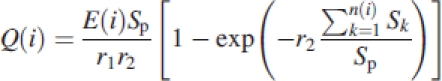1

where Q(i) the fresh biomass created at time step i; r₁ and r₂ are blade resistance and a competition factor, respectively; E(i) is the average, potential of biomass production during GC(i); n(i) is the number of green leaves during the ith GC; S_k the blade area of the kth leaf; S_p is the ground projection area of the leaf surface.

Each type of organ, o (blade, b; sheath, s; internode, e; cob, f; tassel, m), is defined by specific endogenous parameters: a sink strength P, and an expansion law defined as a beta law with two parameters a and b.

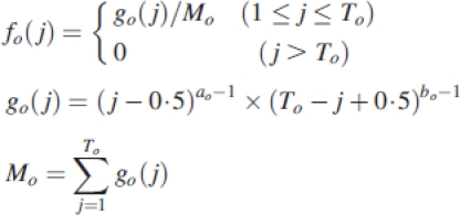2

f_o(j) is an organ-specific sink variation function of j age. A normalization constraint Σ_j=1^t_o f_o(j)=1 is set, with to the expansion duration of organ, o. The parameters a_o and b_o vary with organ type. Organ sink strengths are generally normalized by setting blade sink value to 1, as a reference for all the other relative organs sinks.

During the general parameterization of 12 model parameters by optimization (Table 1), only one parameter (B_o, eqn 3) is optimized to define the beta function for each organ type, and its two parameters a_o and b_o are subsequently derived from B_o by iteration using the constraints a_o+b_o=5 and

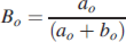3

For a given chronological age, the equation expressing the demand in biomass at a given GC i can be written:

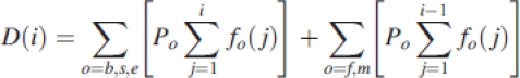4

with D(i) the demand of all plant organs at the ith GC, P_o and f_o are the sink strength and the sink variation function of the organ type o, respectively. At a given GC i, the biomass increment of an organ having the age j is equal to:

5

Biomass accumulation for this organ is:

6

As a consequence of these model concepts, organ size is variable because it depends on resources and the number and strength of sinks that share these resources at a given time. The model is deterministic (final organ number and crop duration are fixed), although model versions exist that use stochastic organogenetic principles as well as resource feedbacks of organogenesis, such as tiller production. GREENLAB permits graphic, three-dimensional outputs for each simulation time step, enabling animation and post-simulation analyses, e.g. light distribution in the canopy.

Table 1.

Parameters of GREENLAB adjusted by optimization

Parameter	Comment
Pb	Blade sink strength; Pb is set to 1
Ps	Sheath sink strength
Pe	Internode sink strength
Ke	Secondary pith sink for short internodes
	Cob sink strength
PfPm	Tassel sink strength (no expansion variation for this)
Bb	Blade sink variation (parameter for the beta law of organ expansion)
Bs	Sheath sink variation
Be	Pith sink variation
Bf	Cob sink variation
r1	Blade resistance depending on leaf area
r2	Competition factor (i.e. leaf overlapping effect on PET)

Parameter optimization

Optimization uses a generalized least squares method that was described by Zhan et al. (2003). As reported in detail by Guo et al. (2006), two methods were used for optimization of GREENLAB parameters: single fitting using only one target file (a priori a final description of plant architecture and organ weight) and multi-fitting using several target files describing plants architecture and biomass at different growth stages.

Field experiments

Four field experiments (expts 2000, 2001, 2003A and 2003B) were conducted at the China Agricultural University (CAU) (39°50′N, 116°25′E). Another field experiment with identical design (expt 2005) was conducted at the Quzhou experiment station (36°52′N, 115°1′E) located in the North China Plain. Experiment schedules are described in Table 2.

Table 2.

2000, 2001, 2003 and 2005 field experiment schedules

Experiment	Sowing date	Emergence	Harvest	Duration (d)
2000	8 May	18 May	5 August	89
2001	20 April	1 May	5 August	107
2003A	19 May	26 May	13 August	86
2003B	29 June	4 July	13 September	75
2005	23 May	29 May	8 August	77

Maize cultivar ND108 (Zea mays L., DEA cultivar) seeds were sown 0·6 m apart in north-south oriented rows that were 0·6 m apart. The resulting plant population (28·000 plants ha^–1) was about half of that commonly used by local farmers and was chosen to minimize competition among plants, the aim here being to analyse growth and organogenesis of individual plants.Seeds were sown on 8 May in 2000 (expt 2000), 20 April in 2001 (expt 2001), 19 May in 2003 (expt 2003A), 29 June (expt 2003B) and 23 May (expt 2005) (Table 2). Emergence was recorded between 5 and 10 d after sowing, depending on seasonal conditions. The experiments had four replications in 2000, 2001 and 2005; and five replications in 2003A and 2003B. A randomized, complete block design was used. One plant was collected per replication and sampling date. At both sites, the soil was a sandy clay loam (Aquic Cambisol) previously managed as meadow. The plots were irrigated and fertilizer inputs were such as to avoid any mineral and water limitation to plant growth. Weeds were removed by hand to avoid any herbicide effects on plant growth. No plant disease, pest or stress symptoms were observed. The meteorological data needed to calculate potential evapotranspiration (PET) (daily mean, minimum and maximum air temperature, mean relative humidity, wind speed, actual sunshine hours) were recorded at a field weather station located on the experimental site for expts 2000–2003, but were obtained from a standard weather station located 10 km from the experimental field at the Quzhou site in 2005.

Field measurements on plants

During crop development, destructive sampling was periodically done on individual plants in order to characterize growth and organogenesis. Only above-ground organs were collected. Samples were taken on 12 dates in 2000, seven in 2001, 14 in 2003A, 18 in 2003B and nine in 2005. To prevent water loss during measurements, plants were dug out with roots and soil and transported to the laboratory for measurements [width, length and fresh weight (f. wt) of leaf sheaths; length, width, area and f. wt of leaf blades; diameter, length and f. wt of internodes; dimensions and f. wt of cob and tassel]. These measurements were done on all existing metamers on the sample plants. The date of onset of senescence was recorded for each metamer in order to estimate leaf life span. Blade area was measured using a LI-COR 3100 leaf area meter (Lincoln, NB, USA).

For each sampling date, the observed organ f. wt and dimension data was input in a target file which subsequently served as reference for statistical optimization of model parameters. Details of target file structure and optimization procedures were described by Guo et al. (2006).

Simulation experiments and statistics

A series of modelling exercises was carried out to evaluate the variability of optimized model parameters when adjusted to different phenotypes produced by the same genotype. The phenotype variability was that observed among individual plants within a population (replications), among environments (seasons) and among development stages of the same crop. Simulation experiments were conducted in four steps.

1. For the five experiments (seasons), the model parameters described in Table 1 were optimized for individual plants (replications) on one target file each describing observations made at maturity [single fitting procedure as described by Zhan et al. (2003) and Yan et al. (2004)]. Optimized parameters were compared among replications and seasons.

2. In order to analyse the stability of the parameters across different developmental stages, target files containing the means of replications were established for GCs 8, 18 and 30. Parameter fitting was thus performed for the vegetative phase alone (GCs 1–8), all phases until nearly silking (GCs 1–18) or all phases until nearly maturity (GCs 1–30). Growth stages GCs 8, 18 and 30 were considered consecutively as the final stage.

3. A simplified set of target files was established for expt 2000, containing three metamers for GC 8 (2, 5, 7) and GC 18 (6, 11, 17), and all 21 metamers for GC 30. These three target files were then used simultaneously for parameter optimization (multi-fitting; Guo et al., 2006).

4. The model parameters obtained with the simplified target files for 2000 were validated with 2001, 2003A, 2003B and 2005 field observations.

Regression and variance analyses were conducted with Sigma Plot V.9 (SYSTAT Inc.) and StatGraphics (Centurion Inc.) softwares.

RESULTS AND DISCUSSION

Field observations

Regardless of seasons and year, the maize crop produced nearly the same number of metamers (20–22 at maturity). In Fig. 1A, metamer number is expressed along thermal time using T_b=8 °C as base temperature). Plants developed at about the same rate regardless of season, as indicated by the similar amount of thermal time required for the production of new metamers. As plants in expt 2003A were already harvested at 30 GC, but harvested in the other seasons at 33 GC, comparisons among seasons used 30 GC as common reference. In Fig. 1B, average values of PET per GC are presented for the 30th GC in each of the five crops. Potential evapotranspiration or PET, which is the environmental variable driving biomass acquisition in GREENLAB, varied strongly within and among seasons. Note that PET for expt 2003B was particularly different since this experiment was carried out between July and September whereas the others were carried out from May to August (Table 2).

Fig. 1.

(A) Number of metamers as a function of thermal time and (B) average values of PET per growth cycle. The insert in (A) shows that the production rate of metamers was not affected by sowing date.

Average plant biomass at the 30th GC varied between 1042 and 2063 g plant^–1 depending on the season, and was particularly low in 2003B and 2005 (Table 3). This can be explained with accelerated crop development due to higher temperatures during these two seasons, resulting in shorter absolute duration of the crop (Table 2) and of each GC (Table 3), whereas the thermal duration per GC was unaffected. Mean PET per day, considered the driving force of transpiration and biomass assimilation in GREENLAB, was very similar among seasons. This translated into reduced, cumulative PET per GC in 2003B and 2005. In fact, final plant biomass at the 30th GC was positively correlated across seasons with the mean, thermal duration per GC [biomass (g plant^–1)=–659+158 PET (mm GC^–1), with R²=0·75 and P=0·01].

Table 3.

Shoot fresh biomass at GC 30 (near maturity) and mean thermal time (TT) per day at 8 °C base temperature, potential evapotranspiration (PET) per day and per growth cycle (GC), and the absolute and thermal duration per GC for five seasons

Season	Shoot fresh biomass (g plant–1)	TT d–1 (Tbase=8) °C (°C d–1)	PET d–1 (mm)	PET GC–1 (mm)	Time GC–1 (d)	TT GC–1 (°C d–1)
2000	2063	16·8	5·5	15·2	2·8	47·0
2001	1755	14·6	5·2	16·1	3·1	45·3
2003A	1553	16·9	5·4	15·0	2·8	47·3
2003B	1042	18·3	4·9	11·3	2·3	42·1
2005	1286	19·7	5·4	11·8	2·2	43·3

The lower plant biomass in 2003B and 2005 seasons is explained by the higher temperatures, which made GCs shorter and reduced PET per GC.

Biomass vs. PET GC^–1 correlation is y=158x – 659, with R²=0·75 and P=0·01.

Figure 2 provides details of fresh biomass development observed during the five seasons. Above-ground biomass accumulation was continuous, whereas that for vegetative plant parts (without cobs and tassels) ceased at about the time when the last (21st) metamer had been developed (the fact that the inflorescences themselves are composed of numerous metamers undergoing branching and metamorphosis is disregarded here).

Fig. 2.

(A) Shoot and (B) vegetative fresh weight for the five seasons, plotted against growth cycles. Means of four replications.

Because GREENLAB does not use empirical partitioning tables but instead allocates fresh biomass to competing sinks, this study gave particular emphasis to biomass distribution observed among organs and organ types at different developmental stages of the plant (Fig. 3). During vegetative growth (GC 8), virtually all biomass was located in leaf blades and sheaths, but showed a continuously decreasing trend. At nearly silking stage (GC 18), almost half of biomass was present in internodes and most of the reminder in leaf blades and sheaths, with only very little biomass in cobs and tassels. At GC 30 (nearly maturity), between 35 % and 50 % of fresh biomass was located in cobs and the reminder divided in about equal proportion between internodes and leaf+sheath.

Fig. 3.

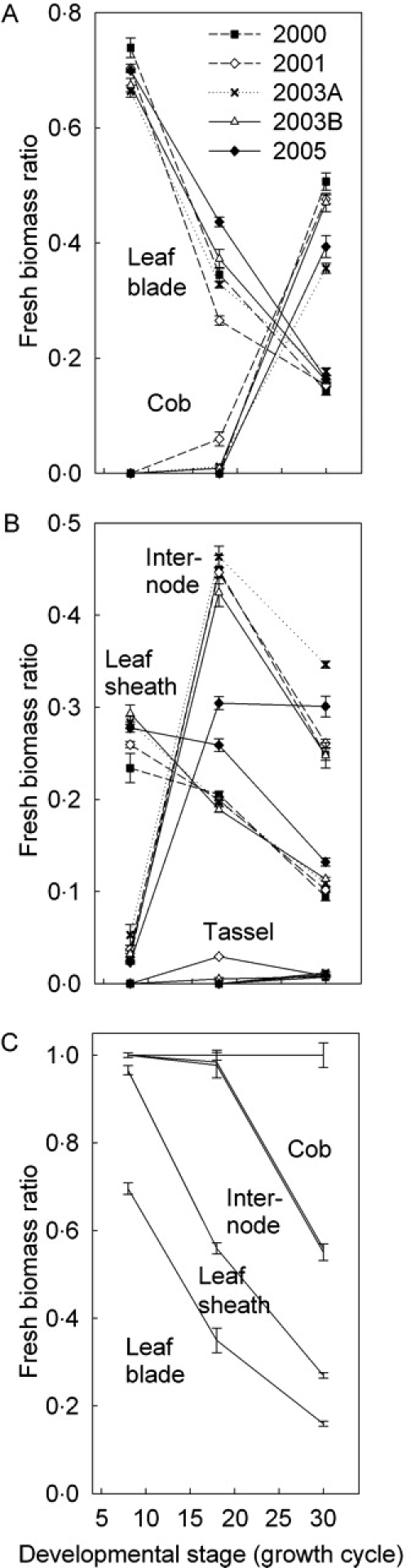
Ratio of organ (leaf blade, sheath, internode, cob, tassel) fresh weight over above-ground fresh weight at three developmental stages (GC 8; GC 18, about silking; GC 30, maturity) during five seasons: (A) leaf blade and cob, means of four replications; (B) intenode, leaf sheath and tassel, means of four replications; (C) stacked, inter-annual means for five seasons. Labels in this graph refer to open spaces (differences) between lines. What appears to be a double line in (C) actually encloses the very small fraction of tassel biomass. Error bars indicate standard error of mean.

The experimental error among plants of a population (replications) for biomass ratios among organ types was small, but significant differences were observed among years. Specifically, plants had less internode biomass and more sheath biomass in 2005, which might be due to sampling errors (e.g. incomplete separation of sheaths from internodes).

The stacked representation of the data in Fig. 3C demonstrates that whenever a new organ type appeared (initially leaf+sheath, then internodes, then cob; the biomass of tassels is negligible), it became the dominant sink. This resulted in a succession of descending lines that were roughly parallel, or (as an alternative interpretation) converging towards a common point on the x axis. The latter interpretation would imply that when a new, dominant sink appeared, the proportions among the already existing ones were preserved. This allometric, highly simplified view of sink relationships is formalized in GREENLAB using the model's sink strength parameters (Table 1).

Model parameter variation among single plants of a population

The comparison of variation of observed variables and model parameters has its limits because they do not behave in the same way, even where they have a similar function (case of mass allometries among organs vs. sink strength parameters of GREENLAB). Allometries such as those presented in Fig. 3 and Table 4 are simple biomass ratios, whereas the model's sink strength parameters govern a cumulative partitioning process. The biomass ratios resulting from this cumulative process may thus be different from the partitioning ratios implemented with the sink strength parameters. These differences are further enhanced by the organ type-specific site-filling kinetics (or expansion laws; Guo et al., 2006) governed by the sink variation parameters (Table 1). It is therefore not useful to compare the absolute ranges of variation of observed variables and model parameters, and this analysis is limited to relative coefficients of variance (CV%), expressed as percentage of variable or parameter means (Table 4).

Table 4.

Coefficients of variance (CV%) among plants of a population (replications, n=4) and among cropping seasons (n=5) for directly observed biomass variables, observed allometric variables and optimized model parameters at about grain maturity (GC=30)

Variable or parameter	Coefficients of variance among plants of a population (replications, n=4), as % of mean						Variance among seasons (n=5) CV%	Inter- vs. intra-seasonal CV% ratio
	2000 CV%	2001 CV%	2003A CV%	2003B CV%	2005 CV%	Mean, intra-seasonal CV%
Variables measured directly on plants
Leaf blade biomass	5·3	7·1	4·1	11·9	6·8	7·0	19·4**	2·77
Leaf sheath biomass	5·5	4·0	10·9	9·9	13·4	8·7	14·4**	1·66
Internode biomass	12·0	9·7	7·5	3·7	12·5	9·1	17·7**	1·95
Cob biomass	6·2	17·6	13·2	5·2	10·1	10·5	22·5**	2·14
Mean	7·3	9·6	8·9	7·7	10·7	8·8	18·5	2·13
Observed allometric mass ratios
Leaf blade/above-ground	10·1	4·3	7·1	2·3	6·7	6·1	7·9*	1·29
Leaf sheath/above-ground	9·7	4·6	5·6	3·0	6·7	5·9	12·8*	2·18
Internode/above-ground	5·2	3·4	2·2	11·0	7·5	5·9	15·1**	2·58
Cob/above-ground	5·9	3·2	4·9	6·7	9·8	6·1	14·3**	2·34
Mean	7·7	3·9	5·0	5·8	7·7	6·0	12··5	2·10
Optimized model parameters
Ps (Sheath sink strength)	2·5	4·5	2·2	3·3	4·1	3·3	6·9	2·09
Pe (internode sink str.)	9·7	2·7	4·6	8·1	8·9	6·8	9·2	1·35
Ke (pith sink strength)	12·9	15·4	13·0	12·7	12·5	13·3	15·3	1·15
Pf (cob sink strength)	9·3	9·9	10·0	7·2	7·8	8·8	12·7	1·44
Pm (tassel sink strength)	8·5	11·2	8·3	8·7	9·5	9·2	12·1	1·31
Bb (blade sink variation)	8·2	11·7	7·5	9·1	8·6	9·0	10·7	1·19
Bs (sheath sink variation)	7·5	10·7	8·3	8·2	8·4	8·6	9·6	1·12
Be (pith sink variation)	9·7	12·2	2·6	11·2	9·1	9·0	10·1	1·12
Bf (cob sink variation)	6·0	12·2	4·6	8·2	3·7	6·9	8·4	1·22
r1 (leaf blade resistance)	4·9	7·8	5·6	5·5	5·7	5·9	8·2	1·39
r2 (competition coeff.)	8·4	11·6	9·0	8·3	8·7	9·2	9·1	0·99
Mean	8·0	10·0	6·9	8·2	7·9	8·2	10·2	1·31

**, P<0·01; *, P<0·05; all other values are not significantly different.

When comparing plant individuals of a population in a given season (representing replications in the experimental design), quite similar values for CV% were observed for absolute mass variables (8·8 %), allometric mass variables (ratios) (6·0 %) and model parameters (8·2 %). It is not surprising that allometric variables varied slightly less than less than absolute mass variables, because internal mass ratios tend to be more stable than absolute mass, at least in the absence of major stresses or other deforming factors. For example, the harvest index of cereals (grain dry weight over above-ground dry weight at maturity) is remarkably stable across very different levels of yield (Echarte and Andrade, 2003).

It is also not surprising that the model parameters on average showed an intermediate variance compared with absolute and allometric variables, because they were fitted to the different individuals observed, and because some were of allometric nature (namely, the sink-strength parameters) and some were related to whole-plant functioning (e.g. resistance parameters). It should be noted, however, that the highly derived (or more abstract) model parameters governing the organ-type specific sink kinetics did not vary much more than the other parameters. Model parameters describing ‘hidden’ or hypothetical properties that are in nature distant from observable reality generally carry a risk of poorly reproducible behaviour.

The largest parameter variance was observed for pith sink variation K_e. Internodes do not only grow in length but also in mass per unit length and in diameter, probably due to reserve accumulation (true secondary growth of stems does not occur in monocots). Although necessary for accurate simulation of maize growth, this parameter stands for a poorly defined and possibly quite variable process, and thus varied more than the other parameters.

Model parameter variation among seasons

This exercise served to evaluate the stability of model parameters when confronted with plant variability caused by different environments (seasons), as opposed to variability among plants grown in the same environment.

Observed, absolute biomass varied much more among seasons (on average, CV%=18·5) than among individuals of a population (replications; CV%=8·8) (Table 4). To a lesser degree, this was also true for allometric variables (12·5 vs. 6·0 %). Model parameters, however, varied only slightly more among seasons (CV%=10·2) than among replications (CV%=8·2). As a whole, inter-seasonal variation of observed variables was 2·1-fold greater than inter-plant variation, whereas inter-seasonal variation of model parameters was only 1·3-fold greater than inter-plant variation. Consequently, the model removed (and thus, explained) a substantial part of the inter-seasonal variation observed. (Evidently, the model could not explain any variation among plants within a season because environmental inputs were identical.) Since PET (driving assimilation) and air temperature (driving phenology) were the only environmental variables considered, it is concluded that these two variables were a suitable choice for the simulation of inter-annual variability of the growth and architecture of a maize crop not limited by water and nutrients.

Model parameter variation among developmental stages of the crop

To analyse the stability of the parameters across different developmental stages, parameter fitting was performed using the target files for the vegetative phase (GC 8), near-silking stage (GC 18) and near-maturity (GC 30). Growth stages GC 8, GC 18 and GC 30 were consecutively considered as the final stage. The variance of the resulting parameter values was compared with that of observed, allometric mass ratios at GC 8, GC 18 and GC 30. These ratios are the result of the previous, cumulative partitioning history of the crop.

Very strong variability was observed during most seasons for allometric mass relationships, particulary those that related organ biomass to above-ground biomass (Table 5). This was expected because as discussed in the previous section, new sinks (internode, cob) appear in the course of phenology and marginalise the previously existing sinks. Allometric mass relationships among vegetative organ types (sheath/blade, internode/blade) were more stable. This analysis could not be extended to reproductive organs because their presence was limited to the last developmental stages (grain filling and maturation) only.

Table 5.

Coefficients of variance (%CV) among growth stages (growth cycle, GC) for observed, allometric mass relationships and for optimized model parameters during each of five cropping seasons

Observed variable or parameter, GCs used	Variable or parameter variation among growth stages (GC), as % of mean fortwo or three different growth stages (CV%)
	2000	2001	2003A	2003B	2005	Mean
Observed, allometric mass ratio
Blade/above-ground, GC 8, 18 and 30	83·9	90·1	75·4	74·0	61·8	77·0
Internode/above-ground, GC 18 and 30	40·7	37·1	20·4	37·2	0·8	27·2
Sheath/above-ground, GC 18 and 30	50·3	52·0	54·5	56·1	35·5	49·7
Internode/blade, GC 18 and 30	20·2	0·83	23·0	20·6	63·6	25·7
Sheath/blade, GC 18 and 30	34·7	33·8	19·2	25·6	34·4	29·5
Model parameter
Ps (sheath sink strength), GC 18 and 30	19·5	8·3	21·4	7·6	10·3	13·4
Pe (internode sink strength), GC 18 and 30	9·6	1·9	12·0	11·2	9·2	8·8
Ke (pith sink strength), GC 18 and 30	9·9	8·3	10·7	7·6	10·3	9·4
Bb (blade sink variation), GC 8, 18 and 30	7·3	7·9	4·3	9·9	15·0	8·9
Bs (sheath sink variation), GC and 18 and 30	11·7	12·3	9·0	8·0	6·8	9·6
Be (pith sink variation), GC 18 and 30	5·6	19·6	11·9	5·5	3·0	9·1
r1 (leaf blade resistance), GC 8, 18 and 30	9·4	9·5	8·1	8·9	11·1	9·4
r2 (competition coefficient), GC 8, 18 and 30	12·1	8·8	7·2	8·5	9·5	9·2

The growth stages are GC 8 (vegetative), GC 18 (about silking) and GC 30 (about maturity).

For GC 8, variables/parameters involving internodes were not considered because this organ was absent.

Variables/parameters involving cobs and tassels were not considered at all because they were present only at GC 30.

Remarkably, fitting of model parameters for the three different phenological periods (GCs 1–8, 1–18 and 1–30) gave much lower parameter variance as compared to the observed allometries. On average across the five seasons, the CV% of all model parameters was below 10, indicating that developmental stage had only small effects on these parameters. As for the analysis of allometric ratios, this analysis did not include model parameters governing reproductive sinks because of their presence during a limited (terminal) period.

Model multi-fitting with a simplified data set

In a previous study (Guo et al., 2006), it was demonstrated that simultaneous multi-fitting of model parameters using target files for several developmental stages, as opposed to observations at maturity only, greatly improves model performance, and in particular the accuracy of organ expansion kinetics. On the other hand, the use of many complete target files (describing observations on all metamers on a specific date) results in an unreasonably large experimental effort. In the following, the results of a compromise is presented based on the use of a complete target file on the mature crop (GC 33) and one target file each for GC 8 (vegetative) and GC 18 (nearly silking), the latter two files containing observations on only three metamers (instead of eight or 18 metamers). Only the 2000 data set was used for parameterization, and the four other experiments were used to validate the model parameters. A simulation resulting from the simplified, multi-fitting procedure is shown in Fig. 4.

Fig. 4.

Simulations resulting from the application of the multi-fitting technique using a simplified set of target files (expt 2000). Horizontal bars: simulated, fresh biomass distribution among metamers at GC 8 (insert), GC 18 and GC 33. ×, Observations used for parameter optimization. No observations on the other GCs were used for parameterization, but simulations for those GCs were of similar quality (not presented).

Simulation of biomass distribution among metamers and among organs produced by a metamer for the 2000 experiment was reasonably accurate for GC 18 and GC 33 except for an underestimation of cob mass. The poor simulation of organs that dramatically change their water content, such as cobs or senescing leaves, highlights a general problem encountered with the model, caused by the simulation of fresh biomass only. A new version distinguishing between dry matter and water is in progress. Another source of parameterization error for cobs was the use of only one observation (on GC 33) for this organ, which made it impossible to fully capture its growth kinetics. Not fully satisfactory was also the simulation of organ mass during early vegetative stages (e.g. GC 8), for similar reasons, because only very few observations on vegetative plants were used (three metamers at GC 8). Model parameterization procedures using reduced data sets for specific growth stages should thus attribute different weight to the various target files in order to avoid distortions. A certain degree of distortion is inevitable, however, because GREENLAB is a mathematical model that does not attribute specific parameters or functions to individual metamer positions, as this is done in other architectural models described elsewhere (Prusinkiewicz et al., 1988; Drouet, 2003, Drouet and Pagès, 2003; Evers et al., 2006), but instead generates weight distributions across metamers in a continuous process with one single, aggregate function and one common set of parameters governing organ relative sink strength and filling kinetics (Yan et al., 2004; Guo et al., 2006). The parameter values obtained with the simplified target files are compared in Table 6 with those obtained with all available target files. The values and their standard deviation were similar for both methods.

Table 6.

Comparison of parameter values, standard deviation and coefficient of variation resulting from the multi-fitting optimization technique applied to total and simplified target files (case of expt 2000)

	Data set using all available observations			Simplified data set using three stages
Parameter	Value	s.d.	CV (%)	Value	s.d.	CV (%)
Pb (Blade sink strength)	1	–	–	1	–	–
Ps (Sheath sink strength)	0·70	0·02	2·9	0·75	0·03	4·0
Pe (internode sink str.)	2·17	0·08	3·7	2·69	0·12	4·5
Ke (pith sink strength)	0·33	0·09	27·3	0·31	0·08	25·8
Pf (cob sink strength)	202	33·1	16·4	217	30·4	14·0
Pm (tassel sink strength)	2·13	0·11	5·2	3·05	0·29	9·5
Bb (blade sink variation)	0·40	0·01	2·5	0·36	0·03	8·3
Bs (sheath sink variation)	0·53	0·02	3·8	0·42	0·03	7·1
Be (pith sink variation)	0·79	0·02	2·5	0·76	0·02	2·6
Bf (cob sink variation)	0·62	0·03	4·8	0·55	0·03	5·5
r1 (leaf blade resistance)	354	18·7	5·3	300	18·4	6·1
r2 (competition coeff.)	3·34	0·43	12·9	3·99	0·54	13·5

Using the parameters obtained with the simplified procedure for observations made in expt 2000, the field observations in expts 2001, 2003A, 2003B and 2005 were predicted (Fig. 5.). Simulation errors for above-ground biomass, leaf area and stem height, aggregated for all metamers present at a given stage, were generally small as indicated by the clear linearity and slopes similar to 1 for the simulation-observation correlations. Significant (P<0·05) deviations of simulation vs. prediction correlations from the 1:1 relationship were only observed for leaf area for expts 2001 and 2003B (over-estimation of slope parameter). Prediction of final cob biomass for the four seasons was also reasonably good (R²=0·79, slope parameter 1·13; Fig. 5D), although the kinetics of cob filling were poor because dehydration effects were not considered (kinetics not presented).

Fig. 5.

Validation of GREENLAB outputs across all developmental stages for 2001, 2003A, 2003B and 2005, using parameter values calibrated on expt 2000 (simplified data set, multi-fitting technique): (A) above-ground, fresh biomass; (B) leaf area per plant; (C) stem height (sum of all internode lengths); (D) cob fresh biomass at GC 30 (near physiological maturity). In (A–C) data for various phenological stages were pooled; in (D) only the final biomass of cobs is presented. Symbols are data points, lines are regressions. For linear regressions, none of the intercepts of linear regressions differed significantly (P<0·05) from 0, and none of the slopes except those in 2001 (B) and 2003A (B) differed significantly from 1.

A three-dimensional representation of model outputs for two contrasting seasons (2003A and 2003B), using the parameters generated with the simplified data set for 2000 (Table 6), is shown in Fig. 6. The 2003B season had lower PET per unit GC than 2003A because of higher temperatures (but similar PET per day), which led to hastened plant development and thus, lower biomass (Table 3). The morphological differences between the smaller 2003B plants and the larger 2003A plants concern most organs, but are particularly visible for leaves on the earlier metamers (produced when differences between the two seasons were most pronounced), as well as for overall plant height and cob size. The dynamic, three-dimensional image files of GREENLAB can be used for agronomic applications such as radiative balances (Sinoquet et al., 1998) and the design of optimized plant architecture (plant types; Donald, 1968; Dingkuhn et al., 1991). Such applications are currently being explored by running the model for plant populations of different stand densities.

Fig. 6.

Three-dimensional visualization of simulated maize plant at GC 30 in experiments 2003A and 2003B and corresponding, simulated growth dynamics.

Overall assessment of parameter stability

This study demonstrated that the parameters of the functional–structural plant model GREENLAB show remarkable stability for maize across seasonal environments characterized by different temperatures and PET. These two variables are the driving forces of development rate and biomass accumulation in the model. The comparison of parameter variation among plants of a common population (replications) and among populations (seasons) showed that the model does not explain inter-plant variance, which translates roughly proportionally into parameter variance. On the other hand, it did explain in large part the inter-seasonal variance of phenotype, as indicated by the comparatively small parameter variation associated with it. This kind of model behaviour is generally expected from any good agronomic plant model, but was achieved here with a mathematical, architectural model that simulates very few physiological processes and feedbacks.

In contrast to other architectural plant models such as those based on L-Systems (Evers et al., 2006), GREENLAB uses a single type of equation to describe the sink capacity and growth kinetics of all plant organs (which only differ in parameter values), and a single set of parameter values for organs produced by different metamers. Consequently, the size and shape of individual organs is not forced with individual parameter values (Prusinkiewicz et al., 1988; Drouet, 2003, Drouet and Pagès, 2003), nor with empirical functions implementing effects of developmental stage or metamer rank as practised elsewhere (Evers et al., 2006). This raises the question of parameter stability across developmental stages or metamer ranks, which might be associated with different organ behaviour. In fact, Tivet et al. (2001) showed that leaf length and width proportions of rice change slightly with developmental stage, Dingkuhn (1996) reported that nitrogen availability strongly affects leaf-stem assimilate partitioning, and Dingkuhn et al. (2006) reported that the timing of sorghum internode elongation is sensitive to both metamer number stage and photoperiodic signals.

The present analysis of variance of model parameter values according to developmental stages (GC) was necessarily restricted to vegetative plant organs because reproductive organs are not present during much of the plant life cycle. (Although the model generally uses stage-independent parameter values, stage-specific values were determined here to study their stability.) For leaf blades, sheaths and internodes, empirical parameter values varied little among growth stages, as compared with the large variation in allometric variables observed among developmental stages in the field. This result demonstrates that at least some of the apparent changes in organ expansion properties between growth stages was explained by the intrinsic rules of the modelling process (which simulates inter-organ competition for assimilates) and thus, did not require metamer- or stage-specific parameters. But there are clearly limits to parameter stability (or genericity) resulting from changes in plant behaviour either in the course of phenology (e.g. vernalization or photoperiod effects) or triggered by stress events. To simulate these, the model must be sensitive to such triggers and implement the physiological response, which necessarily disrupts the linearity of the simulation process. GREENLAB so far has no provision for such mechanisms but a version, simulating water-limited growth, is being developed that enables feedback of drought on biomass growth and partitioning.

In the Introduction the inherent difficulty of extracting genetic (generic) information from phenotypic (variable) observations was evoked. Physiological growth models are mostly assembled from ex-ante knowledge on generic mechanisms, which are then parameterized using experimentally established parameters and, as a last step, for the remaining ‘black boxes’, with phenotype information obtained from a variety of environments. GREENLAB, by contrast, uses very little ex-ante information (e.g. ‘PET drives transpiration drives assimilation’; ‘development is a function of thermal time’) and a small set of laws on recurrent morphogenetic processes (e.g. periodicity of organogenesis, principles of site filling and resource sharing), while generating many of the plant's behavioural characteristics with a statistical optimization procedure. It is thereby assumed that the plant system functions in a continuous, coherent and linear way. Interestingly, this mathematical approach resulted in remarkable parameter stability (although the environments considered probably were too similar to test the concept to its limits). A logical next step will be to apply the model to different genotypes in order to study its parameter's genotypic variation and, ultimately, their relationships with genetic information.

CONCLUSIONS

This study aimed at evaluating the ability of GREENLAB, a mathematical and architectural plant growth model, to overcome plant phenotypic plasticity encountered in a multi-season experiment and to retrieve systemic and generic plant parameters. The analysis of parameter stability among plants of a population sharing the same environment and among populations grown in different environments indicated that the model explains some of the inter-seasonal variability of phenotype (parameters vary much less than the phenotype itself), but not the inter-plant variability (parameter and phenotype variability are similar). Parameter variability among developmental stages was small, indicating that the equations and parameter values were largely development-stage independent. On the basis of these results, a simplified set of plant observations was developed that helps reduce the experimental effort for model parameterization while providing similar goodness-of-fit as that obtained with a much larger data set. The authors suggest that the high level of parameter stability in GREENLAB should be used to conduct comparisons among genotypes and ultimately, genetic analyses. Some model improvements, including the distinction between fresh and dry biomass, are also suggested.

LITERATURE CITED

- Allen RG, Pereira LS, Raes D, Smith M. FAO, Rome: 1998. Crop evapotranspiration. Guidelines for computing crop water requirements. FAO Irrigation and Drainage Paper No. 56. [Google Scholar]
- Dingkuhn M. Modelling concepts for the phenotypic plasticity of dry matter and nitrogen partitioning in rice. Agricultural Systems. 1996;52:383–397. [Google Scholar]
- Dingkuhn M, de Vries FWTP, de Datta SK, van Laar HH. Direct seeded flooded rice in the tropics. Manila, Philippines: International Rice Research Institute; 1991. Concepts for a new plant type for direct seeded flooded tropical rice; pp. 17–38. [Google Scholar]
- Dingkuhn M, Luquet D, Quilot B, de Reffye P. Environmental and genetic control of morphogenesis in crops: towards models simulating phenotypic plasticity. Australian Journal of Agricultural Research. 2005;56:1289–1302. [Google Scholar]
- Dingkuhn M, Luquet D, Kim HK, Tambour L, Clément-Vidal A. EcoMeristem, a model of morphogenesis and competition among sinks in rice. 2. Simulating genotype responses to phosphorus deficiency. Functional Plant Biology. 2006;33:325–337. doi: 10.1071/FP05267. [DOI] [PubMed] [Google Scholar]
- Donald CM. The breeding of crop ideotypes. Euphytica. 1968;17:385–403. [Google Scholar]
- Drouet JL. MODICA and MODANCA: modelling the three-dimensional shoot structure of graminaceous crops from two methods of plant description. Field Crops Research. 2003;83:215–222. [Google Scholar]
- Drouet JL, Pagès L. GRAAL: a model of growth, architecture and carbon allocation during vegetative phase of the whole maize plant: model description and parameterisation. Ecological Modelling. 2003;165:147–173. [Google Scholar]
- Echarte L, Andrade FH. Harvest index stability of Argentinean maize hybrids released between 1965 and 1993. Field Crops Research. 2003;82:1–12. [Google Scholar]
- Evers JB, Vos J, Fournier C, Andrieu B, Chelle M, Struik PC. An architectural model of spring wheat: evaluation of the effects of population density and shading on model parameterization and performance. Ecological Modelling. 2006 doi:10.1016/j.ecolmodel.2006.07.042. [Google Scholar]
- Guo Y, Ma YT, Zhan ZG, Li BG, Dingkuhn M, Luquet D, et al. Parameter optimization and field validation of the functional–structural model GREENLAB for maize. Annals of Botany. 2006;97:217–230. doi: 10.1093/aob/mcj033. [DOI] [PMC free article] [PubMed] [Google Scholar]
- Hammer GL, Kropff MJ, Sinclair TR, Porter JR. Future contributions of crop modelling – from heuristics and supporting decision making to understanding genetic regulation and aiding crop improvement. European Journal of Agronomy. 2002;18:15–31. [Google Scholar]
- Luquet D, Dingkuhn M, Kim HK, Tambour L, Clément-Vidal A. EcoMeristem, a model of morphogenesis and competition among sinks in rice. 1. Concept, validation and sensitivity analysis. Functional Plant Biology. 2006;33:309–323. doi: 10.1071/FP05266. [DOI] [PubMed] [Google Scholar]
- Prusinkiewicz P, Lindenmayer A, Hanan J. Developmental models of herbaceous plants for computer imagery purposes. Computer Graphics. 1988;22:141–150. [Google Scholar]
- Reymond M, Muller B, Leonardi A, Charcosset A, Tardieu F. Combining quantitative trait loci analysis and an ecophysiological model to analyse the genetic variability of the responses of maize leaf growth to temperature and water deficit. Plant Physiology. 2003;131:664–675. doi: 10.1104/pp.013839. [DOI] [PMC free article] [PubMed] [Google Scholar]
- Ritchie JT, NeSmith DS. Temperature and crop development. In: Hanks RJ, Ritchie JT, editors. Modeling plant and soil systems. Madison, WI: American Society of Agronomy Monograph No. 31; 1991. pp. 5–29. [Google Scholar]
- Sinoquet H, Thanisawanyangkura S, Mabrouk H, Kasemspa P. Characterization of the light environment in canopies using 3D digitizing and image processing. Annals of Botany. 1998;82:203–212. [Google Scholar]
- Tardieu F. Virtual plants: modelling as a tool for the genomics of tolerance to water deficit. Trends in Plant Science. 2003;8:9–14. doi: 10.1016/s1360-1385(02)00008-0. [DOI] [PubMed] [Google Scholar]
- Tivet F, da Silveira Pinheiro B, de Raïssac M, Dingkuhn M. Leaf blade dimensions of rice (Oryza sativa L. and Oryza glaberrima Steud.): relationships between tillers and main stem. Annals of Botany. 2001;88:507–511. [Google Scholar]
- de la Vega AJ, Hall AJ, Kroonenberg PM. Investigating the physiological bases of predictable and unpredictable genotype by environment interactions using three-mode pattern analysis. Field Crops Research. 2002;78:165–183. [Google Scholar]
- Wright SD, McConnaughay KDM. Interpreting phenotypic plasticity: the importance of ontogeny. Plant Species Biology. 2002;17:119–131. [Google Scholar]
- Yan HP, Kang MZ, de Reffye P, Dingkuhn M. A dynamic, architectural plant model simulating resource-dependent growth. Annals of Botany. 2004;93:591–602. doi: 10.1093/aob/mch078. [DOI] [PMC free article] [PubMed] [Google Scholar]
- Yin XY, Stam P, Kropff MJ, Schapendonk AHCM. Crop modeling, QTL mapping, and their complementary role in plant breeding. Agronomy Journal. 2003;95:90–98. [Google Scholar]
- Zhan ZG, de Reffye P, Houllier F, Hu BG. Fitting a functional–structural growth model with plant architectural data. In: Hu BG, Jaeger M, editors. Proceedings of Plant Growth Modeling and Applications (PMA'03) Beijing: Tsinghua University Press/Springer-Verlag; 2003. pp. 236–249. [Google Scholar]