Using relative utility curves to evaluate risk prediction

Summary

Because many medical decisions are based on risk prediction models constructed from medical history and results of tests, the evaluation of these prediction models is important. This paper makes five contributions to this evaluation: (1) the relative utility curve which gauges the potential for better prediction in terms of utilities, without the need for a reference level for one utility, while providing a sensitivity analysis for missipecification of utilities, (2) the relevant region, which is the set of values of prediction performance consistent with the recommended treatment status in the absence of prediction (3) the test threshold, which is the minimum number of tests that would be traded for a true positive in order for the expected utility to be non-negative, (4) the evaluation of two-stage predictions that reduce test costs, and (5) connections among various measures of prediction performance. An application involving the risk of cardiovascular disease is discussed.

1. Introduction

The use of patient medical history and additional testing to make treatment decisions is common in medical practice. For example, consider the following choices faced by an asymptomatic person contemplating treatment for cardiovascular disease, where the specified level of risk for decision-making needs to be determined:

1. Treat based on prediction model for baseline variables Receive treatment only if the estimated risk of cardiovascular disease based on a prediction model for baseline variables (age, smoking, systolic blood pressure, and total cholesterol) is greater than or equal to a specified level,

2. Treat based on prediction model for baseline variables and result of additional test Receive treatment only if the estimated risk of cardiovascular disease based on a prediction model involving baseline variables and results of an additional test for high density lipoprotein (HDL) is greater than or equal to a specified level,

3. Treat none. Receive no treatment, without estimating risk of cardiovascular disease,

4. Treat all. Receive treatment, without estimating risk of cardiovascular disease,

5. Treat based on a two-stage prediction model for baseline variables and result of additional test On the first stage, receive treatment if the estimated risk based on the model with only baseline variables is above an intermediate range, which is a clinical “gray zone”, receive no treatment if the estimated risk is below this intermediate range, and undergo a second stage if the estimated risk is in the intermediate range. On the second stage, receive an additional test for HDL and receive treatment only if the new estimated risk based on a prediction model involving the baseline variables plus the additional test for HDL is greater than or equal to a specified level within the intermediate range.

We have two related goals: (i) determine the optimal specified level of risk to use as a threshold with the various treatment options and (ii) choose among treatment options based on costs and benefits, taking into account the possibility of incorrectly specifying costs and benefits.

Purely statistical measures of prediction performance, such as the area under the receiver operating characteristic (ROC) curve, risk classification tables (Cook, 2007), predictiveness curves (Huang, et al 2007), and reclassification summary measures (Pencina, et al 2008), have limited value for choosing among the treatment options because they do not account for costs and benefits.

A more fruitful approach for choosing among the treatment options is to introduce utilities for various outcomes and perform a sensitivity analysis to allow for misspecification of the utilities. This approach is the focus of this paper and will be discussed in more detail in later sections. For now, the following brief background will suffice. A positive prediction (which prompts treatment) is defined as an estimated risk at or above a specified level; a negative prediction (which does not prompt treatment) is defined as an estimated risk below the specified level. The expected utility of prediction is a weighted average (over probabilities of predictions and outcomes) of four basic utilities associated with prediction, namely utilities associated with false and true positive predictions and false and true negative predictions. Perhaps the first formulation of the expected utility of prediction was Peirce (1884).

Related to our first goal, the risk threshold is a scalar function of the four basic utilities of prediction that is the optimal specified level of risk for positive prediction, in the sense of maximizing a person’s expected utility given his four basic utilities of prediction. The formula for risk threshold was derived directly by Pauker and Kassirer (1975) and Gail and Pfeiffer (2005) and is implied by the result of Metz (1978).

Related to our second goal, we choose the treatment option with the highest expected utility. The challenge is how to summarize the sensitivity of the expected utility to misspecification of the risk threshold, which conveniently summarizes the information on utilities. Ideally one would like an easily interpretable function of the expected utility that depends on the four basic utilities of prediction only through the risk threshold, which is not the case with the expected utility by itself. Adams and Hand (1999) and Briggs and Zaretski (2008) proposed functions of expected utility that depend on the four basic utilities only through the risk threshold, but assumed zero utilities for true positives and negatives, which is unrealistic in many medical settings. Vickers et al (2006) proposed the net benefit as a function of the expected utility that depends on the four basic utilities only through the risk threshold without the need for additional assumptions. The net benefit is the number of true positives minus the number of false positives valued in terms of true positives. Computation of net benefit involves setting the difference between utilities of a true positive and a false negative equal to one, as a reference value. Vickers et al (2006) also proposed the decision curve, which is a plot of net benefit versus risk threshold.

This paper makes five contributions. The first is a new function of expected utilities, called the relative utility, that is a function of the four basic utilities only through the risk threshold but, unlike net benefit, does not require a reference value for any utility. In particular, the relative utility is the maximum fraction of expected utility achieved by risk prediction as compared with perfect prediction. A relative utility curve is a plot of relative utility versus risk threshold. The relative utility curve allows investigators to gauge the potential for improved performance with better prediction models while at the same time providing a sensitivity analysis. A second contribution is the relevant region, which is the set of values of performance measure consistent with treatment status in the absence of prediction. The relevant region is useful for restricting the sensitivity analysis. A third contribution is the test threshold, which is the minimum number of tests that would be traded for a true positive in order for the expected utility to be non-negative. The test threshold is useful when the harms of a test are not known precisely. A fourth contribution is the evaluation of the decision option involving two-stage prediction model which, to our knowledge, has not been previously done. The two-stage prediction model has the potential to reduce testing costs with little loss in prediction performance. A fifth contribution is the elucidation of the connections among various measures of prediction performance.

The paper is organized into the following sections: parametrizations, utilities, expected utilities for standard prediction, expected utility for two-stage prediction, risk threshold, decision curves, relevant region, relative utility curves, test threshold, an example, and a discussion.

2. Parametrizations

Throughout this article, we assume a risk prediction model has already been developed. After introducing notation for risk prediction models, we review various sets of parameters that can be used to compute expected utility and hence construct decision or relative utility curves (as discussed in subsequent sections).

2. 1 Prediction models

Let D_i = 0, 1 denote the absence and presence of disease in person i. In diagnostic and screening tests, the absence or presence of disease is a binary indicator. In prospective cohort studies, the absence or presence of disease refers to no occurrence or occurrence of disease by a specified time. Let $z_i^{\ast }$ denote a vector of risk factors for person i. The prediction model for person i can be generally written as $pr(D_i=1\mid z_i^{\ast },\beta )$ where β is a vector of parameters. Examples include logistic regression for a binary outcome or a proportional hazards model for disease occurrence by a given time.

If the risk prediction model involves many parameters relative to the number of individuals, there is a concern about bias from overfitting, namely using the same data to estimate parameters and evaluate performance. To avoid overfitting bias, parameters should be estimated in a training sample and performance should be evaluated in an independent test sample. We let pr (D_i = 1 | z_i, β̂) denote the estimated risk in the test sample, where z_i is a vector of risk factors for person i in the test sample (as distinguished from $z_i^{\ast }$ which applies to the training sample), and β̂ is the estimate of the parameter vector obtained from the training sample.

Let J = j denote cutpoints for the estimated risk pr(D_i = 1| z_i, β̂) over all individuals in the independent test sample, ordered from smallest to largest values. (Tied estimated risks can be ordered arbitrarily). The cutpoints can correspond to either individuals or intervals. For example suppose pr(D_i = 1| z_i, β̂) = 0.20, 0.10, 0.15, 0.30 for persons i = A, B, C, D, respectively. There are four possible cutpoints based on individuals: j = 1, 2, 3, 4 corresponding to persons B, C, A, D, respectively. One might also consider two cutpoints based on intervals, for example, j = 1 corresponding to [0.00, 0.18) which encompasses risk for persons B and C, and j = 2 corresponding to [0.18, 0.30), which encompasses risk for persons A and D. Our convention is that J ≥ j is a positive prediction and J < j is a negative prediction for a given value of j.

2.2 Risk

One set of parameters that can be used to compute expected utility is

r_j = pr(D = 1| J = j) = risk,

w_j = pr(J = j). = weight.

The risk is the probability of disease at cutpoint j of the estimated risk. The weight is the probability the estimated risk equals j. These parameters can be estimated using prospective follow-up data.

If the cutpoints (indexed by j) correspond to intervals, the estimated weight is ŵ_j = n_j/N, where n_j is the number of subjects in interval j. The predicted estimated risk, r̂_PREDj = Σ_iεjpr(D = 1| z_i, β̂)/n_j, is the average estimated risk in the interval. The observed estimated risk, denoted r̂_OBSj, equals the fraction with disease among subjects in interval j if the outcome is binary; and one minus the Kaplan Meier estimate of survival in interval j if the outcome is time of disease occurrence. Compared to the observed estimated risk, the predicted estimated risk has smaller confidence intervals but requires the model to be correctly specified.

If the cutpoints (indexed by j) correspond to individuals at increasing estimated risk, the estimated weight is ŵ_j = 1/N, where N is the number of persons, and the estimated risk for the j^th person ordered by estimated risk is r̂_j = r̂_PREDj = pr(D = 1| z_j, β̂). Usually the average of r̂_PREDj among persons within an interval of estimated risks is compared to the observed estimate of risk for that interval. If the estimates are close, the prediction model is thought to give a reasonable fit and the predicted estimated risks are said to be well-calibrated.

Sometimes risk is summarized via a predictiveness curve (Huang et al 2007), which plots r̂_j versus Σ_s≤j ŵ_s, which is the estimated cumulative distribution function for estimated risk.

2.3 Receiver operating characteristic (ROC) curves

Another set of parameters that can be used to compute expected utility is

FPR_j = pr(J ≥ j|D = 0) = false positive rate, also called one minus specificity,

TPR_j = pr(J ≥ j|D = 1) = true positive rate, also called sensitivity,

π = pr(D = 1) = probability of disease at a given time, also called prevalence.

The false (true) positive rate is the probability of positive prediction among those without (with) disease. These parameters can be estimated using either case-control data (with an exogenous estimate of π) or data from prospective follow-up with a binary or survival endpoint. Generally, predicted and observed estimates can be obtained by substituting {ŵ_j, r̂_PREDj} and {ŵ_j, r̂ OBS_j}, respectively, into

$$FP{R}_j=\frac{{\Sigma }_{s\ge j}(1-r_s)w_s}{{\Sigma }_s(1-r_s)w_s},TP{R}_j=\frac{{\Sigma }_{s\ge j}{r}_s{w}_s}{{\Sigma }_s{r}_s{w}_s}\text{and}\pi ={\Sigma }_s{r}_s{w}_s.$$ (1)

When disease outcome is survival to a given time, observed estimates of FPR and TPR can be computed by substituting the Kaplan Meier estimate of r_j into (1), which is a special case, apparently not previously recognized, of Heagerty et al (2000).

With case-control data (or prospective follow-up with a binary outcome), the observed estimate of FPR_j equals the fraction of subjects with J ≥ j among all subjects without disease, and the observed estimate of TPR_j equals the fraction of subjects with J ≥ j among all subjects with disease. To ensure accuracy of FPR and TPR in a case-control analysis, the severity of disease in cases and spectrum of conditions in controls that could give a positive test result, should be similar to the population in which the test will ultimately be used (Ransahoff and Feinstein, 1978).

An ROC curve is a plot of estimates of {FPR_j, TPR_j} for all cutpoints j. The higher the true positive rate for a given false positive rate, the better the performance of the risk prediction. For perfect classification, FP̂R_j = 0 and TP̂R_j = 1 for some value of j.

2.4 Predictive values

A third set of parameters that can be used to compute expected utility is

PPV_j = pr(D = 1| J ≥ j) = positive predictive value,

NPV_j = pr(D = 0| J < j) = negative predictive value,

η_j = pr(J ≥ j) = proportion positive.

The positive predictive values is the probability of disease among those with positive prediction. The negative predictive value is the probability of no disease among those with negative prediction. Predicted and observed estimates are obtained by substituting {ŵ_j, r̂_PREDj} and {ŵ_j, r̂ OBS_j}, respectively into

$$NP{V}_j=\frac{{\Sigma }_{s<j}(1-r_s)w_s}{{\Sigma }_{s<j}{w}_s},PP{V}_j=\frac{{\Sigma }_{s\ge j}{r}_s{w}_s}{{\Sigma }_{s\ge j}{w}_s},{\eta }_j={\Sigma }_{s\ge j}{w}_s.$$ (2)

When disease outcome is binary, the observed estimate of NPV_j equals the fraction of subjects without disease among subjects with J < j, and the observed estimate of PPV_j equals the fraction of subjects with disease among subjects with J ≥ j.

3. Utilities

We specify that persons predicted as positive receive treatment and persons predicted as negative do not receive treatment. Treatment could be a drug, surgery, or further testing that might lead to a drug or surgery. Each possible combination of prediction (negative and positive) and disease status (0, 1) is associated with a utility. These utilities of prediction and testing are denoted

U_TP = utility of a true positive when risk prediction is positive, treatment is given, and disease is present or will develop,

U_FP = utility of a false positive when risk prediction is positive, treatment is given, but disease is absent or will not develop,

U_FN = utility of a false negative when risk prediction is negative, no treatment is given, but disease is present or will develop,

U_TN = utility of true negative, when risk prediction is negative, no treatment is given, and disease is absent or will not develop,

U_Test = utility (monetary cost or harm) from a test to obtain information on baseline variables,

U_TestA = utility (monetary cost or harm) from an additional test.

Our convention is that utilities are negative if they are detrimental. In the context of a questionnaire to estimate the risk of colorectal cancer, Gail and Pfeiffer (2005) set U_FN = -100 for the possibility of death and morbidity due to failing to detect colorectal cancer, U_FP = -1 for the risk of bleeding or perforation of the colon, U_TP = -11 for the risk of bleeding or perforation of the colon and the lowered chance of death or morbidity from colorectal cancer due to early detection, and U_TN = 0 as a reference value. See Pauker and Kassirer (1975) for an example in which utilities are survival probabilities. For later development the following definitions are needed:

P = U_TP - U_FN = profit for positive prediction among those with disease,

L = U_TN - U_FP = loss for positive prediction among those without disease,

C = - U_Test/P = cost of test for baseline variables per unit profit,

C_A = - U_TestA/P = cost of additional test per unit profit.

The terminology “profit” and “loss” come from Peirce (1884). The profit P is the difference in utilities from making a positive instead a negative prediction of disease among those with disease. The loss L is the negative (to make it a positive number that is subtracted in later equations) of the difference in utilities from making a positive instead of a negative prediction of disease among those without disease. In the aforementioned example from Gail and Pfeiffer (2005), P = - 11 - (- 100) = 89 and L = 0 - (-1) = 1. Because testing cost is detrimental, U_Test and U_TestA are negative, so C and C_A are positive.

4. Expected utility for prediction

The expected utility for prediction (which is one-stage unless otherwise noted) corresponding to cutpoint j is the average of the utilities of each combination of prediction and disease status weighted by the probabilities of occurrence, plus the utility of testing to obtain information on the variables used for prediction,

$$U_j=pr(J\ge j,D=1)U_{TP}+pr(J<j,D=1)U_{FN}+pr(J<j,D=0)U_{TN}+pr(J\ge j,D=0)U_{FP}+U_{\text{Test}}.$$ (3)

Following Metz (1978), the expected utility in terms of ROC curve parameters is

$$\begin{array}{cc}\hfill U_j=& \pi TP{R}_j{U}_{TP}+\pi (1-TP{R}_j)U_{FN}+(1-\pi )(1-FP{R}_j)U_{TN}+(1-\pi )FP{R}_j{U}_{FP}+U_{\text{Text}}.\hfill \\ \hfill =& [\pi TP{R}_{j}P-(1-\pi )FP{R}_{j}L]+[U_{FN}\pi +U_{TN}(1-\pi )]+U_{\text{Text}}.\hfill \end{array}$$ (4)

Formulations of the expected utility in terms of risk parameters and positive predictive values can be found in Appendix A. The formula for the expected utility for prediction involving baseline variables plus the result of an additional test is similar to (4) except for different values for FPR_j and TPR_j and the addition of U_TestA.

5. Expected utility for two-stage prediction

We also derived a formula for the expected utility for two-stage prediction discussed in the Introduction. Suppose the first stage corresponds to interval S = [a, b-1] which defines intermediate risk with the values of a and b determined by clinical considerations that lead to a “grazy zone” when treatment is debatable. Let pr(S) denote the probability the estimated risk from the initial prediction is in interval S and let pr(S|D = d) denote the probability of the same event conditional on disease status. For the second stage let K = k denote cutpoints for estimated risk from the prediction model involving the baseline variables and results of the additional test among persons with initial estimated risk in S. Let $r_k^{\ast }=pr(D=1\mid K=k,S)$ and let $w_k^{\ast }=pr(K=k\mid S)$. The expected utility for two-stage prediction (in which a positive prediction corresponds to either a first stage cutpoint greater than or equal to b or a second stage cutpoint greater than or equal to k among subjects in the intermediate range on the first stage) is

$$\begin{array}{cc}\hfill U_k^{\ast }=& \pi TP{R}_k^{\ast }{U}_{TP}+\pi (1-TP{R}_k^{\ast })U_{FN}+(1-\pi )(1-FP{R}_k^{\ast })U_{TN}+(1-\pi )FP{R}_k^{\ast }{U}_{FP}+U_{\text{Test}}+pr\left(S\right)U_{\text{Test}\mathrm{A}},\text{where}\hfill \\ \hfill FP{R}_k^{\ast }& =pr(J\ge b\mid D=0)+pr(K\ge k\mid S,D=0)pr(S\mid D=0)\hfill \\ \hfill & =FP{R}_b+\{\sum _{s\ge k}(1-r_s^{\ast }){\omega }_s^{\ast }∕\sum _s(1-r_s^{\ast }){\omega }_s^{\ast }\}pr(S\mid D=0),\hfill \\ \hfill TP{R}_k^{\ast }& =pr(J\ge b,D=1)+pr(K\ge k,D=1\mid J\in S)]pr(S\mid D=1)\hfill \\ \hfill & =TP{R}_b+\{\sum _{s\ge k}{r}_s^{\ast }{\omega }_s^{\ast }∕\sum _s{r}_s^{\ast }{\omega }_s^{\ast }\}pr(S\mid D=1).\hfill \end{array}$$ (5)

The reduction in costs associated with two-stage prediction arises from the multiplication of U_TestA by pr(S). The formula for computing true and false positives in terms of risk is based on (1). Because K is constructed from different predictors than J, it is possible to consider values of k larger than b - 1, which could occur if the additional test considerably improves prediction in the intermediate risk group.

6. Risk threshold

As mentioned previously, a person’s risk threshold, which we denote R, is a scalar function of U_TP, U_FN, U_TN, and U_FP that determines the cutpoint for calling a result positive that maximizes expected utility. As shown in Appendix B (which is based on proofs in the literature and an extension to two-stage prediction when the maximum expected utility is associated with a risk threshold on the second stage),

$$R=\text{risk threshold}=\frac{L}{L+P}=\frac{1}{1+P∕L}.$$ (6)

The risk threshold can thought of as either the level of risk at which a person is indifferent between treatment or not (Appendix B) or a function of P/ L, which is the number of false positives that a person would trade for each true positive. As used in later formulas, one starts with R and uses it to find the optimal cutpoint j where the person’s risk is greater than or equal to R (and hence maximizes expected utility). This process is summarized using the following notation:

$$j\left(R\right)=\text{smallest value of}j\text{such that}{r}_j\ge R.$$ (7)

7. Decision curves

The drawback to using expected utility to evaluate risk prediction performance is the need to specify U_TP, U_FP, U_FN, (with U_TN = 0 as a reference), which makes a sensitivity analysis difficult. Decision curves (Vickers et al, 2006) simplify the sensitivity analysis because they depend on U_TP, U_FP, U_FN, and U_TN only though a single number, the risk threshold. The original presentation of decision curves involved a step-by-step format for clinicians. We present an algebraic formulation, which serves as a springboard for the subsequent derivations. We start with expected utilities of treating none (all classified as negative) and treating all persons (all classified as positive),

$$U_{\text{None}}=\pi U_{FN}+(1-\pi )U_{TN},$$ (8)

$$U_{\text{All}}=\pi U_{TP}+(1-\pi )U_{FP},$$ (9)

respectively. From (4), (8), and (9),

$$\begin{array}{cc}\hfill U_j-U_{\text{None}}=& \pi TP{R}_{j}P-(1-\pi )FP{R}_{j}L+U_{\text{Test}}\hfill \\ \hfill =& P[\pi TP{R}_j-(1-\pi )FP{R}_j\frac{R}{1-R}-C],\hfill \end{array}$$ (10)

$$\begin{array}{cc}\hfill U_j-U_{\text{All}}=& \pi TP{R}_{j}P-(1-\pi )FP{R}_{j}L-\pi P+(1-\pi )L+U_{\text{Test}}\hfill \\ \hfill =& P[-\pi (1-TP{R}_j)+(1-\pi )(1-FP{R}_j)\frac{R}{1-R}-C],\hfill \end{array}$$ (11)

$$U_{\text{All}}-U_{\text{None}}=P[\pi -(1-\pi )\frac{R}{1-R}].$$ (12)

In the theory of decision curves, (10) and (12) with P = 1 and j = j(R) are defined as the net benefit of risk prediction versus treat none and the net benefit of treat all versus treat none, respectively. Setting P = 1 as reference level means that net benefit is measured in units of true positives. Setting j = j(R) means evaluation is at risk threshold R. Consequently, the net benefit is the number of true positives minus the number of false positives valued as true positives, evaluated at risk threshold R Decision curves are plots of estimates of (10) and (12) versus R.

8. Relevant region

In some settings, there is a clear recommendation for either treatment or no treatment in the absence of prediction. This is increasingly becoming the case as measures of quality care are promulgated and management guidelines are issued by professional societies and panels. Although clinical judgment is always an important component of medical practice, many guidelines and measures of quality care represent attempts to bring more uniformity to medical practice in order to avoid unwarranted variation in therapy. This is the case with guidelines that have been issued regarding the management of hypercholesterolemia, blood pressure, and glycated hemoglobin in diabetics.

In these settings the decision to recommend or not recommend treatment in the absence of prediction provides important information that restricts the range of a sensitivity analysis. In this regard we define the relevant region as the values of a performance measure consistent with the recommended treatment status in the absence of prediction. If treatment is given in the absence of prediction then U_All > U_None, and thus the relevant regions are R < π and slope of the ROC curve < 1, which can be derived from (8) and (9) and from (20) in Appendix B, respectively. Conversely if treatment is not given in the absence of prediction, U_All ≤ U_None, and thus the relevant regions are R ≥ π and the slope of the ROC curve ≥ 1. Relevant regions are indicated by arrows in the figures. In these settings, the sensitivity analysis for risk threshold should not extend beyond the relevant region.

9. Relative utility curves

We propose an enhancement of decision curves that we call relative utility curves. Relative utility curves provide information on how much risk prediction contributes to clinical utility relative to perfect prediction. In contrast to decision curves, there is no need to set any utility equal to a reference value. A first step in the derivation of relative utilities is to define the utility of perfect prediction,

$$U_{\text{Perfect}}=\pi P+\pi U_{FN}+(1-\pi )U_{TN},$$ (13)

which is obtained by substituting TPR_j = 1, FPR_j = 0, and U_Test = 0 into (4). The utility of no prediction equals the larger of U_None and U_All. Based on the relevant region, the relative utility (RU) is the ratio of the maximum utility of the prediction model (versus no prediction) to the utility of perfect prediction (versus no prediction),

$$RU(R,C)=\{\begin{array}{cc}\frac{U_{j\left(R\right)}-U_{\text{All}}}{U_{\text{Perfect}}-U_{\text{All}}},\hfill & \text{if}R<\pi ,\hfill \\ \frac{U_{j\left(R\right)}-U_{\text{None}}}{U_{\text{Perfect}}-U_{\text{None}}},\hfill & \text{if}R\ge \pi .\hfill \end{array}\phantom{\}}$$ (14)

In the terminology of medical decision-making, U_j - U_None is called the net expected value of clinical information and U_Perfect - U_None is the called the expected value of perfect clinical information (Weinstein et al, 1980). Because U_Perfect - U_None = π P and U_Perfect - U_All = (1 - π) L, we can use (10) and (11) to write (14) as

$$RU(R,C)=\{\begin{array}{cc}[1-FP{R}_{j\left(R\right)}]-[1-TP{R}_{j\left(R\right)}]\frac{\pi }{1-\pi }\frac{1-R}{R}-\frac{1-R}{R}\frac{C}{(1-\pi )},\hfill & \text{if}R<\pi ,\hfill \\ TP{R}_{j\left(R\right)}-\frac{1-\pi }{\pi }\frac{R}{1-R}FP{R}_{j\left(R\right)}-\frac{C}{\pi },\hfill & \text{if}R\ge \pi .\hfill \end{array}\phantom{\}}$$ (15)

If the ROC curve is concave the relative utility is increasing from R = 0 to R = π, maximum at R = π, and decreasing from R = π to R = 1. See Appendix C for a heuristic justification. Relative utility can also be expressed using parameters involving risk or predictive values (Appendix D).

9.1 Estimation

When estimating the relative utility in (15) via the risks in (1), it is helpful to note that j ≥ j(R) corresponds to r_j ≥ R. For example suppose there are six individuals whose risks after ordering are r₁ = 0.01, r₂ = 0.02, r₃ = 0.04, r₄ = 0.16, r₅ = 0.17, and r₆ = 0.19 corresponding to disease status of 0, 1, 0, 0, 1, 1, respectively. If the risk threshold is R = 0.10, the region for a positive prediction consists of all individuals with r_j ≥ 0.10. Therefore the predicted estimates are TP̂R_j(R) = (0.16 +0.17 + 0.19) / (0.01 + 0.02 + .004 + 0.16 + 0.17 + 0.19) = 0.88 and FP̂R_j(R) = (0.84 +.083 + 0.81) / (0.99 + 0.98 + 0.96 + 0.84 + 0.83 + 0.81) =0.46, and the observed estimates are TP̂R_j(R) = 2/3 and FP̂R_j(R) = 1/3. These estimates of FPR_j(R) and TPR_j(R) are substituted into (15) with R = 0.10. A relative utility curves is a plot of the estimate of (15) versus R. Predicted estimates yield smoother curves with less variability but require the validity of the model.

To measure variability of relative utility curves and avoid overfitting, we recommend randomly splitting the data into training and test samples multiple times (Michiels et al, 2005) and computing standard errors from the distribution of relative utilities in the random test samples. If there are few parameters relative to the number of subjects, so overfitting is less of a concern, standard errors may be computed by bootstrapping.

9.2 Relationship to odds ratio

To gain insight, suppose the ROC curve is derived by setting the odds ratio for disease versus no disease (OR) to be a constant greater than one regardless of the cutpoint. As derived in the Appendix E and illustrated in Figure 1, the relative utility curves have the same shape regardless of the prevalence of disease. Importantly, as shown in Figure 1, large values of OR in terms of standard epidemiology, such as 3, translate into small relative utilities. The maximum possible relative utility is $(\sqrt{OR}-1)∕(\sqrt{OR}+1)$ , when R = π.

Figure 1.

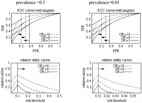
ROC and relative utility curves derived from simple model in which odds ratio for disease versus no disease (OR) is constant regardless of cutpoint. Arrows point to relevant regions. Testing cost is zero. Tangents from ROC curve relate to Appendix C. Derivation of curves is found in Appendix E.

9.3 Prognostic value of an additional risk factor

A measure of the prognostic value of an additional risk factor for one-stage prediction is the difference in relative utilities,

$$DRU(R,C_A)=R{U}_1(R,C+C_A)-R{U}_0(R,C),$$ (16)

where RU₀ (R, C; π) is the relative utility of the risk prediction model based on baseline variables, RU₁ (R, C + C_A) is the relative utility of risk prediction model for baseline variables plus the additional risk factor, and C cancels from the difference. A measure of the prognostic value of an additional risk factor in the two-stage prediction model is the difference in relative utilities,

$$DR{U}^{\ast }(R,C_A)=R{U}_1^{\ast }(R,C,C_A)-R{U}_0(R,C),$$ (17)

where $R{U}_1^{\ast }(R,C,C_A)$ is the relative utility based on the risk prediction model fit to the subset of subjects as well as the original risk prediction model (Appendix F).

10. Test threshold

Another contribution is what we call the test threshold, which is the minimum number of tests that have to be traded for a true positive in order for the expected utility (or relative utility) to be non-negative. The test threshold is basically a lower bound for 1/C = -P/U_Test or 1/C_A = -P/U_TestA for prediction based on testing to be worthwhile. It is particularly useful if U_Test is not known precisely, but a bound is useful. The formula for test threshold can be readily derived when the relevant range is R ≥ π (Appendix G), giving

$$\text{test threshold when the relevant range is}R\ge \pi =\{\begin{array}{cc}1∕\left\{\pi RU(R,0)\right\},\hfill & \text{for test of baseline variables,}\hfill \\ 1∕\left\{\pi DRU(R,0)\right\},\hfill & \text{for additional test under one-stage prediction,}\hfill \\ pr\left(S\right)∕\left\{\pi DR{U}^{\ast }(R,0)\right\},\hfill & \text{for additional test under two-stage prediction.}\hfill \end{array}\phantom{\}}$$

11. Risk of cardiovascular disease

We return to the example in the Introduction. We fit risk prediction models for cardiovascular disease among 26,478 non-diabetic women in the Women’s Health Study (Ridker et al, 2005, Cook, 2007). Here D = 1 corresponds to cardiovascular disease by year 8 of the study. Because all subjects were followed and only 1.6% of women were censored due to death from causes other than cardiovascular disease and hence excluded, D was treated as a binary variable. If a woman’s estimated risk were above her risk threshold, she would receive treatment with statins. In the absence of a prediction, the vast majority of women would not receive statins, which implies a relevant region of R ≥ π or, equivalently, the slope of the ROC curve ≥ 1.

We investigated two models, Model no HDL, which is a logistic regression with baseline risk factors without HDL, and Model HDL, which is a logistic regression with the additional risk factor of HDL. For two-stage prediction, we considered a subset of persons with estimated risk on the first stage 0.04 and 0.16. Standard errors were computed from 25 bootstrap replications of the data.

Figures 2, 3, and 4 show similar ROC, decision, and relative utility curves, respectively, for Model HDL and Model no HDL. The advantage of the decision and relatively curves over ther ROC curve is the direct connection to the risk threshold. A nice feature of the relative utility curves is that they show the potential for improved prediction. Table 1 presents the differences in relative utility curves and test thresholds associated with various risk thresholds. The following example illustrates how to use the relative utility curve to help decide whether or not to receive additional testing for HDL. We discuss results in terms of both observed estimates (based on fractions of individuals in an interval with disease) and predicted estimates (based on the model estimates for individuals), as defined previously.

Figure 2.

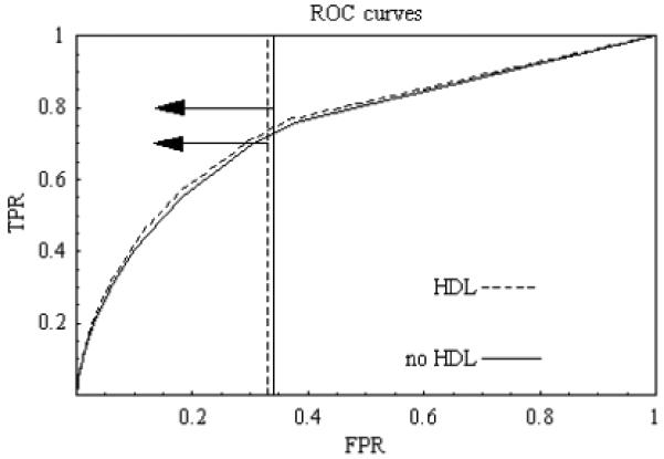
ROC curve for evaluation of risk prediction for cardiovascular disease among all women in the study based on predicted estimates. Prevalence is 0.02. Arrows point to relevant regions. Testing costs are zero.

Figure 3.

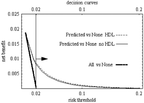
Decision curve for evaluation of risk prediction for cardiovascular disease among all women in the study based on predicted estimates. Prevalence is 0.02. Testing cost are zero. Arrow points to relevant region. “Predicted versus None” refers to equation (10) and “All versus None” refers to equation (12) in the text.

Figure 4.

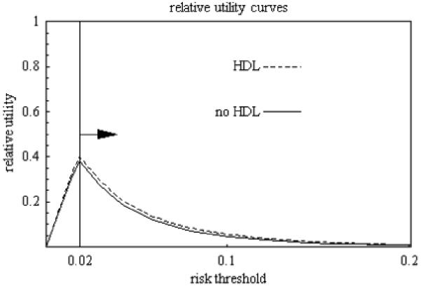
Relative utility curve for evaluation of risk prediction for cardiovascular disease among all women in the study based on predicted estimates. Prevalence is 0.02. Arrow points to relevant regions.

Table 1.

Evaluating risk prediction for cardiovascular disease

risk threshold	model or comparison	type of estimate	relative utility estimate (s.e.)	test threshold estimate (s.e.)
0.04	no HDL	observed	0.207 (0.043)	241	(51)
		predicted	0.206 (0.016)	243	(19)
	HDL	observed	0.228 (0.042)	219	(40)
		predicted	0.227 (0.018)	220	(17)
	difference: 1-stage	observed	0.021 (0.021)	2,371	(2,394)
		predicted	0.021 (0.006)	2,373	(679)
	difference: 2-stage	observed	0.028 (0.017)	220	(138)
		predicted	0.019 (0.008)	317	(128)
0.08	no HDL	observed	0.050 (0.032)	1,009	(642)
		predicted	0.073 (0.011)	686	(103)
	HDL	observed	0.078 (0.032)	641	(262)
		predicted	0.085 (0.013)	590	(87)
	difference: 1-stage	observed	0.028 (0.018)	1,734	(1,080)
		predicted	0.012 (0.005)	4,156	(1,794)
	difference: 2-stage	observed	0.042 (0.021)	144	(71)
		predicted	0.020 (0.009)	299	(133)
0.12	no HDL	observed	0.022 (0.024)	2,308	(2,547)
		predicted	0.031 (0.006)	1, 610	(328)
	HDL	observed	0.024 (0.024)	2,073	(2,101)
		predicted	0.038 (0.007)	1,316	(258)
	difference: 1-stage	observed	0.002 (0.013)	20,066	(104,171)
		predicted	0.007 (0.004)	7,085	(3,800)
	difference: 2-stage	observed	0.014 (0.022)	448	(723)
		predicted	0.014 (0.006)	424	(187)
0.16	no HDL	observed	0.016 (0.014)	3,041	(2,546)
		predicted	0.015 (0.004)	3,384	(993)
	HDL	observed	0.025 (0.015)	1,966	(1,129)
		predicted	0.018 (0.006)	2,709	(814)
	difference: 1-stage	observed	0.009 (0.015)	5,473	(9,088)
		predicted	0.004 (0.004)	13,366	(13,203)
	difference: 2-stage	observed	0.015 (0.028)	396	(722)
		predicted	0.007 (0.005)	813	(506)

Standard errors are in parentheses. Observed estimate is based on fractions with disease; predicted estimate is based on individual estimated risks. One-stage prediction involves additional test in all subjects; two-stage predictions involves additional test only in subjects with estimated risk in intermediate range. Relative utility assumes no test. Test threshold is the number of tests that have to be traded for a true positive for prediction to be worthwhile (i.e. have positive expected utility) at a given risk threshold.

Consider a person with risk threshold R = 0.08, which implies P/L = (1-R)/R = 11.5 false positive predictions of cardiovascular disease would be traded for a true postitive prediction. To maximize expected utility for this person, an estimated risk of cardiovascular disease of 0.08 or greater should be considered as positive indicating treatment, otherwise there would be no treatment. An additional test for HDL increases the observed estimated relative utilities at this risk threshold from 0.050 to 0.078 (a difference of 0.028 with estimated standard error of 0.018) and the predicted estimated relative utility from 0.073 to 0.085 (a difference of 0.012 with an estimated standard error of 0.005). Under one-stage prediction, the observed and predicted estimated test thresholds for HDL testing are 1,734 and 4,156, respectively. For two-stage prediction with intermediate range of 0.04 to 0.16, the observed and predicted estimated test thresholds for HDL testing reduce to 144 for the observed estimate and 299 for the predicted estimate. This minimum of 144 or 299 tests exchanged for a true positive in order to obtain a non-negative expected utility would likely be reasonable for many persons given the low monetary costs and little harm associated with HDL testing. As a sensitivity analysis consider a person with risk threshold of R = 0.12, which implies P/L = (1 - R)/R = 7.3 false positive predictions of cardiovascular disease would be traded for a true positive prediction. To maximize expected utility for this person, an estimated risk of cardiovascular disease of 0.12 or greater should be considered as positive indicating treatment, otherwise there would be no treatment. An additional test for HDL increases the observed estimated relative utility at this risk threshold from 0.022 to 0.024 (a difference of 0.002 with estimated standard error of 0.013) and the predicted estimated relative utility from 0.031 to 0.038 (a difference of 0.007 with an estimated standard error of 0.004). For two-stage prediction with intermediate range of 0.04 to 0.16, the observed and predicted estimated test thresholds for HDL testing are 448 for the observed estimate and 424 for the predicted estimate, which may still seem reasonable given low monetary cost and little harm of HDL testing.

It is also of interest to consider the commonly applied rule to treat for cardiovascular disease if a person’s estimated 8-year risk for cardiovascular disease is greater than 0.16 (equivalent to a 10-year risk greater than 0.20). Based on our previous discussions, this treatment option is only optimal if a person has a risk threshold of 0.16, which implies P/L = (1 - R)/R = 5.25 false positive predictions of cardiovascular disease would be traded for a true positive prediction. In this case, the additional test for HDL increases the relative utility by 0.009 under the observed estimate and 0.004 under predicted estimate. The commonly applied rule refers to one-stage prediction in which the observed and predicted estimated test thresholds for HDL testing are 5,473 and 13,336, respectively. Under two-stage prediction the observed and predicted estimated test thresholds for HDL testing are 396 and 813 respectively. Thus, in terms of HDL testing, the commonly applied rule is less attractive than a rule based on two-stage prediction.

Based on Table 1, we can summarize the sensitivity analysis for HDL testing under two-stage prediction with a first-stage estimated risk in the intermediate range of 0.04 to 0.16. We found that for the range of risk thresholds from 0.04 to 0.16 in the second stage, the observed and predicted estimates of test thresholds for HDL testing were reasonable (with the caveat that the observed estimates have large standard errors and the predicted estimates require the validity of the model).

12. Discussion

This paper proposes using relative utility curves interpreted in the relevant regions and with computation of test thresholds to evaluate one-stage and two-stage prediction rules. Relative utility is an easily interpretable function of expected utility that depends on basic utilities only through risk threshold. To put relative utility curves into perspective versus other contributions related to the use of utilities to evaluate prediction, see Table 2.

Table 2.

Comparison of various utility-based measures for risk prediction

Reference	key formula or contribution
Peirce (1884)	utility of the method	π T P R P - (1 - π) F P R L
Pauker and Kassirer (1975)	threshold	risk threshold R
Metz (1978)	best operating point	optimal slope of ROC curve
Adams and Hand (1999)	loss-difference1,2	sign of differences in models of Uj(R’) - UNone verses R’
Gail and Pfeiffer (2005)	loss ratio	Uj(R) / Uperfect
Vickers et al (2006)	decision curves2	Uj(R) - UNone verses R; U(All) - UNone verses R;
Briggs and Zaretzki (2008)	skill plot1,2	$\{\begin{array}{cc}\frac{U_{\text{No}\text{ne}}-U_j}{U_{\text{No}\text{ne}}}\text{versus}j,\hfill & R^{\prime }\ge \pi ,\hfill \\ \frac{U_{\text{All}}-U_j}{U_{\text{All}}}\text{versus}j,\hfill & R^{\prime }<\pi .\hfill \end{array}\phantom{\}}$
proposed	relative utility curves	$\{\begin{array}{cc}\frac{U_{j\left(R\right)}-U_{\text{None}}}{U_{\text{Perfect}}-U_{\text{None}}}\text{versus}R,\hfill & R\ge \pi ,\hfill \\ \frac{U_{j\left(R\right)}-U_{\text{All}}}{U_{\text{Perfect}}-U_{\text{All}}}\text{versus}R,\hfill & R<\pi .\hfill \end{array}\phantom{\}}$

¹assumes U_TP = U_TN = 0

²with new scale for utilities

U_TP, U_FP, U_TN, U_FN =utilities of true positive, false positive, true negative, false negative, respectively;

FPR = false positive rate; TPR= true positive rate

U_j is the expected utility for interval j under risk prediction model;

P = U_TP - U_FN is profit from positive prediction among diseased

L = U_TN - FP is loss (subtracted) from positive prediction among not diseased

R = L/(L + P) is the risk threshold

R’ is the risk threshold when U_TP = U_TN = 0

U_None is the expected utility of no treatment without a prediction;

U_All is the expected utility of treatment without a prediction;

U_Perfect is expected utility of perfect prediction.

Relative utilities curves can be constructed for any number of additional tests. For example suppose that additional tests A, B, and C are under consideration. One can fit a risk prediction model with baseline variables and results from any subset of A, B, and C. Relative utilities can also be computed for different prediction models using the same variables.

A controversial issue is how to interpret the difference in relative utilities when the standard errors are large. Some would argue that the only quantity of interest is the expected value of the difference in relative utilities. Others would argue that decision-makers should be conservative about introducing new tests, so that for a definitive conclusion the standard errors must be small.

When estimating uncertainty in the relative utility curve, we did not incorporate uncertainty in the risk threshold in addition to the uncertainty in parameter estimates because we are conditioning on the risk threshold. We wanted to estimate relative utility had the risk threshold been at a specified level. Had we wanted to estimate relative utility with an unknown risk threshold, we would have needed to incorporate the uncertainty in the risk threshold. By analogy when computing the uncertainty for an ROC curve one typically conditions on the false positive rate; however when computing the uncertainty of the true positive rate for a test in which no cutpoint has been fixed, one should incorporate the uncertainty in the false positive rate (Greenhouse and Mantel, 1950).

Appendix A

The expected utility can be written using the other sets of parameters besides those for the ROC curve. Following Gail and Pfeiffer (2005), the expected utility in terms of risk parameters is

$$U_j=\sum _{s\ge j}{r}_s{w}_s{U}_{TP}+\sum _{s<j}{r}_s{w}_s{U}_{FN}+\sum _{s<j}(1-r_s)w_s{U}_{TN}+\sum _{s\ge j}(1-r_s)w_s{U}_{FP}+U_{\text{Test}.}$$ (18)

Related to Greenland (2008), the expected utility in terms of predictive values is

$$\begin{array}{cc}\hfill U_j=& {\eta }_{j}PP{V}_j{U}_{TP}+(1-{\eta }_j)(1-NP{V}_j)U_{FN}+(1-{\eta }_j)NP{V}_j{U}_{TN}+{\eta }_j(1-PP{V}_j)U_{FP}+U_{\text{Test}}\hfill \\ \hfill =& {\eta }_j\left\{PP{V}_j\right(P+L)-L\}+[U_{FN}\pi +U_{TN}(1-\pi \left)\right]+U_{\text{Test}}.\hfill \end{array}$$ (19)

which is obtained by substituting η_j PPV_j = πTPR_j and η_j (1 - PPV_j) = (1 - π) FPR_j into (4).

Appendix B

There are various proofs that expected utility of prediction is maximized when risk level for a positive prediction, r_j, equals the risk threshold R.

(a) Following Pauker and Kassirer (1975), consider whether or not treatment should be given if the estimated risk is greater than r_j. There are two arms for the decision tree; (i) estimated risk greater than r_j implies treatment with expected utility of

U_(Treat)j = r_j U_TP + (1-r_j) U_FP

and (ii) an estimated risk greater than r_j implies no treatment with expected utility of

U_(Notreat)j = r_j U_FN + (1-r_j) U_TN

The choice of cutpoint j as optimal occurs if the expected utilities of the two arms are equal, as otherwise, one could increase the utility by shifting the cutpoint. Setting U_(Treat)j = U_(Notreat)j gives r_j = R at the optimum.

(b) Following Gail and Pfeiffer (2005), the maximum of the expected utility, reparametrized as in (18), occurs when the change in expected utility from cutpoint j to j + 1 is zero, i.e.,

U_j - U_j-1 = w_j [(1 - r_j)U_FP - (1 - r_j) U_TN - r_j U_TP - r_j U_FN = 0,

which implies r_j = R.

(c) Following Metz (1978), the maximum of the expected utility parametrized as in (19) occurs when the change in expected utility from cutpoint j to j - 1 is zero, namely,

U_j - U_j-1 = π (TPR_j - TPR_j-1) P - (1 - π) (FPR_j - FPR_j-1) L = 0,

which implies that the slope of the ROC curve at the interval j that maximizes the expected utility is

$$\mathrm{ROC}slop{e}_j\equiv \frac{TP{R}_j-TP{R}_{j-1}}{FPR-FP{R}_{j-1}}=\frac{(1-\pi )}{\pi }\frac{L}{P}=\frac{(1-\pi )}{\pi }\frac{R}{1-R},$$ (20)

which implies r_j = R because

$$\frac{r_j}{1-r_j}=\frac{pr(J=j\mid D=1)pr(D=1)}{pr(J=j\mid D=0)pr(D=0)}=\mathrm{ROC}slop{e}_j\frac{\pi }{1-\pi }=\frac{R}{1-R}.$$ (21)

(d) For the two-stage decision prediction, where k is the interval in the intermediate range defined by S as in (5), the maximum expected utility (assuming it is associated with a risk threshold on the second stage) occurs when the change in expected utility from cutpoint k to k + 1 is zero, namely,

$$\begin{array}{cc}\hfill & U_k^{\ast }-U_{k+1}^{\ast }={\omega }_k[r_k^{\ast }AP+(1-r_k^{\ast })B\}L=0,\text{where}\hfill \\ \hfill & A=\pi pr(S\mid D=1)∕{\Sigma }_s{r}_s^{\ast }{w}_s^{\ast },\hfill \\ \hfill & B=(1-\pi )pr(S\mid D=0)∕{\Sigma }_s(1-r_s^{\ast })w_s^{\ast }.\hfill \end{array}$$ (22)

If the model fits perfectly then A = B = 1, giving $r_k^{\ast }=R$.

Appendix C

We argue geometrically why the relative utility associated with a concave ROC curve reaches a maximum when R = π and monotonically decreases from that point. From (15) and (21), for R ≥ π, RU (R, 0) is the point on the TPR axis intercepted by the line tangent to the ROC curve at j(R). See Figure 1 (top left). For R < π, RU (R, 0) is the point on a horizontal line at TPR = 1 intercepted by the line tangent to the ROC curve at j(R).

Appendix D

We present formulas for relative utility in terms of other parameters. In terms of risk, using (1), we can write (15) as

$$RU(R,C)=\{\begin{array}{cc}\{\sum _{s<j\left(R\right)}(1-r_s)w_s-\sum _{s<j\left(R\right)}{r}_s{w}_s\frac{1-R}{R}-\frac{1-R}{R}C\}\frac{1}{1-\pi },\hfill & \text{if}R<\pi ,\hfill \\ \{\sum _{s\ge j\left(R\right)}{r}_s{w}_s-\frac{R}{1-R}\sum _{s\ge j\left(R\right)}(1-r_s)w_s-C\}\frac{1}{\pi }\hfill & \mathrm{if}R\ge \pi .\hfill \end{array}\phantom{\}}$$ (23)

where s ≥ j(R) corresponds to r_s ≥ R and π = Σ_s r_s w_s. To write relative utility in terms of predictive values, using (2), we first write

$$\begin{array}{c}\sum _{s\ge j}{r}_s{w}_s={\eta }_{j}PP{V}_j,\sum _{s\ge j}(1-r_s)w_s={\eta }_j(1-PP{V}_j),\hfill \\ \sum _{s<j}(1-r_s)w_s=(1-{\eta }_j)NP{V}_j,\sum _{s<j}{r}_s{w}_s=(1-{\eta }_j)(1-NP{V}_j).\hfill \end{array}$$ (24)

Substituting (24) into (23) gives, after some simplification,

$$\begin{array}{c}RU(R,C)=\{\begin{array}{cc}(1-{\eta }_{j\left(R\right)})[NP{V}_{j\left(R\right)}-(1-R)\}(1-R)C\}\frac{1}{(1-\pi )R},\hfill & \text{if}R<\pi ,\hfill \\ \{{\eta }_{j\left(R\right)}(PP{V}_{j\left(R\right)}-R]-C\}\frac{1}{(1-R)\pi }\hfill & \text{if}R\ge \pi .\hfill \end{array}\phantom{\}}\hfill \\ \text{where}\pi ={\Sigma }_j\{{\eta }_{j}PP{V}_j+(1-{\eta }_j)(1-NP{V}_j)\}.\hfill \end{array}$$ (25)

Appendix E

We derive various properties of the class of ROC curves generated by the equation

$$OR=TP{R}_j(1-FP{R}_j)∕\left\{(1-TP{R}_j)FP{R}_j\right\},\mathrm{for}OR>1.$$ (26)

Equation (26) implies

$$TP{R}_j=\left(FP{R}_{j}OR\right)∕\left[(1+FP{R}_j(OR-1)\right].$$ (27)

The slope of this ROC curve is

$$ROCslop{e}_j=\frac{\partial TP{R}_j}{\partial FP{R}_j}=\frac{OR}{{\{1+FP{R}_j(OR-1)\}}^2.}$$ (28)

Rewriting (28) based on the relevant solution to the quadratic equation gives

$$FP{R}_j=\frac{-ROCslop{e}_j-\sqrt{ORROCslop{e}_j}}{ROCslop{e}_j(OR-1)}.$$ (29)

Substituting, from (21), the slope of the ROC curve that maximizes expected utility for risk threshold,

$$\mathrm{ROC}slop{e}_j=\frac{R}{1-R}\frac{1-\pi }{\pi },$$ (30)

into (29) yields FPR_j(R) under this model. Substituting FPR_j(R) under this model into (27) yields TPR_j(R) under this model. Substituting FPR_j(R) and TPR_j(R) under this model into (15) gives, after some algebra, the following relative utility under this model,

$$\begin{array}{c}RU(R,0)=\{\begin{array}{cc}\frac{{\{(1-OR)(1-\pi )+v\}}^2}{{(OR-1)}^3(1-\pi )\pi (1-R)∕R}\hfill & ,\text{if}R<\pi ,\hfill \\ \frac{{\{OR(1-OR)(1-\pi )+v\}}^2}{{(OR-1)}^{3}OR{(1-\pi )}^2,}\hfill & \text{if}R\ge \pi ,\hfill \end{array}\phantom{\}}\hfill \\ \text{where}v=\sqrt{{(OR-1)}^{2}OR(1-\pi )\pi (1-R)∕R}.\hfill \end{array}$$ (31)

From Appendix C, we know the maximum relative utility occurs at R = = π. This motivates writing (1 - R)/R = f (1 - π)/π, where 0 ≤ f, and substituting into (29) which, after some algebra, gives

$$RU(R,0)=\{\begin{array}{cc}\frac{{(-1+\sqrt{fOR})}^2}{(OR-1)f}\hfill & ,\text{if}R<\pi ,\hfill \\ \frac{{(-OR+\sqrt{fOR})}^2}{(OR-1)OR},\hfill & \text{if}R\ge \pi ,\hfill \end{array}\phantom{\}}$$ (32)

indicating that the shape of the relative utilities curves does not depend on disease prevalence. The maximum relative utility is computed by substituting f = 1, which corresponds to R = π, into (32) to yield the maximum value,

$$RU(\pi ,0)=\frac{{\left\{\sqrt{OR}(-1+\sqrt{OR})\right\}}^2}{(OR-1)OR}=\frac{{(-1+\sqrt{OR})}^2}{(OR-1)}=\frac{\sqrt{OR}-1}{\sqrt{OR}+1}.$$ (33)

Appendix F

Based on (5) and (15), the relative utility for the two stage prediction is

$$RU\ast (R,C,C_A)=\{\begin{array}{cc}[1-FP{R}_{k\left(R\right)}^{\ast }]-[1-TP{R}_{k\left(R\right)}^{\ast }]\frac{\pi }{1-\pi }\frac{1-R}{R}-\frac{1-R}{R(1-\pi )}[C+C_{A}pr\left(S\right)],\hfill & \text{if}R<\pi ,\hfill \\ TP{R}_{k\left(R\right)}^{\ast }-\frac{1-\pi }{\pi }\frac{R}{1-R}FP{R}_{k\left(R\right)}^{\ast }-\frac{1}{\pi }[C+C_{A}pr\left(S\right)],\hfill & \text{if}R\ge \pi .\hfill \end{array}\phantom{\}}$$

Appendix G

The formulas for test threshold when R ≥ π are derived from the following: for test of baseline variable,

RU (R, C) = (R, 0) - C/π > 0,

for additional test for one-stage prediction,

DRU (R, C_A) = DRU(R, 0) - C_A/π > 0,

and for additional test for two-stage prediction,

DRU* (R, C_A) = DRU*(R, 0) - C_A/π > 0,

We solve for 1/C, which equals P/U_Test, in the equation corresponding to the test for baseline variables, and obtain - P/U_Test > 1/ {π DRU (R, 0)}, so that 1/ {π DRU (R, 0)} is the minimum number of tests “equivalent” to a true positive. Similarly, we solve for 1/C_A, which equals - P/U_TestA, in the equations corresponding to the additional test.

References

- Adams NM, Hand DJ. Comparing classifiers when the misallocation costs are uncertain. Pattern Recognition. 1999;32:1139–1147. [Google Scholar]
- Briggs WM, Zaretski R. The skill plot: a graphical technique for evaluating continuous diagnostic tests. Biometrics. 2008;64:250–256. doi: 10.1111/j.1541-0420.2007.00781_1.x. [DOI] [PubMed] [Google Scholar]
- Cook NR. Use and misuse of the receiver operating characteristic curve in risk prediction. Circulation. 2007;115:928–935. doi: 10.1161/CIRCULATIONAHA.106.672402. [DOI] [PubMed] [Google Scholar]
- Gail MH, Pfeiffer RM. On criteria for evaluating models for absolute risk. Biostatistics. 2005;6:227–239. doi: 10.1093/biostatistics/kxi005. [DOI] [PubMed] [Google Scholar]
- Greenhouse SW, Mantel N. The evaluation of diagnostic tests. Biometrics. 1950;6:399–412. [PubMed] [Google Scholar]
- Greenland S. The need for reorientation toward cost-effective prediction: Comments on “Evaluating the added predictive ability of a new marker: From area under the ROC curve to reclassification and beyond” by M. J. Pencina et al., Statistics in Medicine. Statistics in Medicine. 2008;27:199–206. doi: 10.1002/sim.2995. Correction. Statistics in Medicine 27, 316. [DOI] [PubMed] [Google Scholar]
- Heagerty PJ,, Lumley T, Pepe MS. Time-dependent ROC curve for censored survival data and a diagnostic marker. Biometrics. 2000;56:337–334. doi: 10.1111/j.0006-341x.2000.00337.x. [DOI] [PubMed] [Google Scholar]
- Huang Y, Pepe MS, Feng Z. Evaluating predictiveness of a continuous marker. Biometrics. 2007;63:1181–1188. doi: 10.1111/j.1541-0420.2007.00814.x. [DOI] [PMC free article] [PubMed] [Google Scholar]
- Michiels S, Koscielny S, Hill C. Prediction of cancer outcome with microarrays: a multiple random validation strategy. Lancet. 2005;365:488–92. doi: 10.1016/S0140-6736(05)17866-0. [DOI] [PubMed] [Google Scholar]
- Pauker SG, Kassirer JP. Therapeutic decision making: a cost-benefit analysis. New England Journal of Medicine. 1975;293:229–234. doi: 10.1056/NEJM197507312930505. [DOI] [PubMed] [Google Scholar]
- Peirce CS. The numerical measure of the success of predictions. Science. 1884;4:453–454. doi: 10.1126/science.ns-4.93.453-a. [DOI] [PubMed] [Google Scholar]
- Pencina MJ, D’Agostino RB, D’Agostino RB, Jr., Vasan RS. Evaluating the added predictive ability of a new marker: From area under the ROC curve to reclassification and beyond. Statistics in Medicine. 2008;27:157–172. doi: 10.1002/sim.2929. [DOI] [PubMed] [Google Scholar]
- Ransahoff DF, Feinstein AR. Problems of spectrum and bias in evaluating the efficacy of diagnostic tests. New England Journal of Medicine. 1978;299:926–930. doi: 10.1056/NEJM197810262991705. [DOI] [PubMed] [Google Scholar]
- Ridker PM, Cook NR, Lee IM, Gordon D, Gaziano JM, Manson JE, Hennekens CH, Buring JE. A randomized trial of low-dose aspirin in the primary prevention of cardiovascular disease in women. New England Journal of Medicine. 2005;352:1293–1304. doi: 10.1056/NEJMoa050613. [DOI] [PubMed] [Google Scholar]
- Vickers AJ, Elkin EB. Decision curve analysis: a novel method for evaluating prediction models. Medical Decision Making. 2006;26:565–574. doi: 10.1177/0272989X06295361. [DOI] [PMC free article] [PubMed] [Google Scholar]
- Weinstein MC, Fineberg HV, Elstein AS, Frazier NS, Neuhauser D, Neutra RR, McNeil BJ. Clinical Decision Analysis. W. B. Saunders; Philadelphia: 1980. [Google Scholar]