Target prediction and a statistical sampling algorithm for RNA–RNA interaction

Abstract

Motivation: It has been proven that the accessibility of the target sites has a critical influence on RNA–RNA binding, in general and the specificity and efficiency of miRNAs and siRNAs, in particular. Recently, O(N⁶) time and O(N⁴) space dynamic programming (DP) algorithms have become available that compute the partition function of RNA–RNA interaction complexes, thereby providing detailed insights into their thermodynamic properties.

Results: Modifications to the grammars underlying earlier approaches enables the calculation of interaction probabilities for any given interval on the target RNA. The computation of the ‘hybrid probabilities’ is complemented by a stochastic sampling algorithm that produces a Boltzmann weighted ensemble of RNA–RNA interaction structures. The sampling of k structures requires only negligible additional memory resources and runs in O(k·N³).

Availability: The algorithms described here are implemented in C as part of the rip package. The source code of rip2 can be downloaded from http://www.combinatorics.cn/cbpc/rip.html and http://www.bioinf.uni-leipzig.de/Software/rip.html.

Contact: duck@santafe.edu

Supplementary information: Supplementary data are available at Bioinformatics online.

1 INTRODUCTION

RNA–RNA binding is a major mode of action of various classes of non-coding RNAs and plays a crucial role in many regulatory processes in all living organisms. Examples include the regulation of translation in both prokaryotes (Narberhaus and Vogel, 2007) and eukaryotes (Banerjee and Slack, 2002; McManus and Sharp, 2002), the targeting of chemical modifications (Bachellerie et al., 2002), insertion editing (Benne, 1992) and transcriptional control (Kugel and Goodrich, 2007). Emerging evidence suggests, furthermore, that RNA–RNA interactions also play a role for the functionality of long mRNA-like ncRNAs (Hekimoglu and Ringrose, 2009). A common theme in many RNA classes, including miRNAs, snRNAs, gRNAs, snoRNAs and in particular many of the procaryotic small RNAs, is the formation of RNA–RNA interaction structures that are much more complex than simple complementary sense–antisense interactions. Thermodynamically, the binding of two RNA molecules A and B can be described by the binding energy ΔG^bind = G_AB − G_A − G_B, i.e. by the difference of the energy of structure formation G_AB of the AB complex and the folding energies G_A and G_B of the two individual RNAs A and B. Thus, the binding or hybridization energy has been widely used as a criterion to predict RNA–RNA interactions (Busch et al., 2008; Rehmsmeier et al., 2004; Tjaden et al., 2006).

The interaction between two RNAs is governed by the same physical principles that determine RNA folding: the formation of specific base pairing patterns whose energy is largely determined by base pair stacking and loop strains. Secondary structures, therefore, are an appropriate level of description to quantitatively understand the thermodynamics of RNA–RNA binding. Just as the general RNA folding problem with unrestricted pseudoknots (Akutsu, 2000), the RNA–RNA interaction problem (RIP) is Non-Polynomial (NP)-complete in its most general form (Alkan et al., 2006; Mneimneh, 2009). Polynomial-time algorithms can be derived, however, by restricting the space of allowed configurations in ways that are similar to pseudoknot folding algorithms (Rivas and Eddy, 1999). The simplest approach concatenates two (or more) interacting sequences and then employs the standard secondary structure folding algorithm with a slightly modified energy model that treats loops containing cut-points as external elements. The software tools RNAcofold (Bernhart et al., 2006; Hofacker et al., 1994), pairfold (Andronescu et al., 2005) and NUPACK (Dirks et al., 2007) subscribe to this strategy. The main problem of this approach is that it cannot predict important motifs such as kissing-hairpin loops. The paradigm of concatenation has also been generalized to the pseudoknot folding algorithm of Rivas and Eddy (1999). The resulting model, however, still does not generate all relevant interaction structures (Chitsaz et al., 2009b; Qin and Reidys, 2007). An alternative line of thought, implemented in RNAduplex and RNAhybrid (Rehmsmeier et al., 2004), is to neglect all internal base pairings in either strand, i.e. to compute the minimum free energy (MFE) secondary structure of hybridization of otherwise unstructured RNAs. RNAup (Mückstein et al., 2006, 2008) and intaRNA (Busch et al., 2008) restrict interactions to a single interval that remains unpaired in the secondary structure for each partner. As a special case, snoRNA/target complexes are treated more efficiently using a specialized tool (Tafer et al., 2009) due to the highly conserved interaction motif. Algorithmically, the approaches mentioned so far are close relatives of the RNA folding recursions given by Zuker and Sankoff (1984).

A different approach was taken independently by Pervouchine (2004) and Alkan et al. (2006), who proposed MFE folding algorithms for predicting the joint structure of two interacting RNA molecules. In this model, “joint structure” means that the intramolecular structures of each partner is pseudoknot free, the intermolecular binding pairs are non-crossing and there is no so-called “zig-zag” configuration (see below for details). The optimal joint structure can be computed in O(N⁶) time and O(N⁴) space by means of dynamic programming (DP). More recently, extensions to the partition function were proposed by Chitsaz et al. (2009b) (piRNA) and Huang et al. (2009) (rip1). In contrast with the RNA folding problem, where minimum energy folding and partition functions can be obtained by very similar algorithms, this is much more complicated for joint structures. The reason is that simple unambiguous grammars are known for RNA secondary structures (Dowell and Eddy, 2004), while the disambiguation of grammar underlying the Alkan–Pervouchine algorithm requires the introduction of a large number of additional non-terminals (which algorithmically translate into additional DP tables). Although the partition function of joint structures can be computed in O(N⁶) time and O(N⁴) space, the current implementations require very large computational resources. Salari et al. (2009) recently achieved a substantial speed-up making use of the observation that the external interactions mostly occur between pairs of unpaired regions of single structures. Chitsaz et al. (2009a), on the other hand, use tree-structured Markov random fields to approximate the joint probability distribution of multiple (≥3) contact regions.

The binding energies provides a useful overall characterization of an RNA–RNA interaction. In many cases, however, the locations of the intermolecular base pairs and the detailed structure of the interaction complex is of crucial importance. Bacterial sRNAs, for example, may either up- or down-regulate mRNA translation depending on the structural changes induced by the interaction (Urban and Vogel, 2007). In particular, in RNA–RNA complexes with multiple interaction sites, i.e. in the class of structures for which the expensive computation of joint structures is necessary, one is interested in the probabilities of hybridization in individual regions and in the interdependencies of alternative conformations, see Fig. 1. The probabilities of the individual building blocks of the DP recursions of Huang et al. (2009), furthermore, do not lend themselves to direct biophysical interpretations (see Supplementary Material).

Fig. 1.

Examples of RNA-RNA interactions structures. The primary interaction region(s) are highlighted in grey in the experimentally supported structural models from the literature: (A) ompA-MicA: (Udekwu et al., 2005); (B) sodB-RyhB: (Geissmann and Touati, 2004); (C) fhlA-OxyS: (Argaman and Altuvia, 2000). Hybridization probabilities computed by rip2 are annotated by black boxes for regions with a probability larger than 10%. In many cases, the computational predictions identify additional hybridization regions that may further stabilize the interaction.

We therefore extend our previous framework in two directions: (i) A modification of the underlying grammar explicitly treats hybrids, i.e. maximal regions with exclusively intermolecular interactions. This allows us to investigate local aspects in much more detail. (ii) A stochastic bracktracing algorithm, in analogy to similar approaches for RNA secondary structure prediction (Ding and Lawrence, 2003; Tacker et al., 1996), which can be used to produce representative structure and to generate samples from the thermodynamic properties. These samples can be useful to assess complex structural features for which it would be too tedious or expensive to design and implement dedicated exact backtracing algorithms.

2 THE HYBRID-PARTITION FUNCTION

2.1 Some basic facts

We briefly review some basic concepts and outline the notation introduced in Huang et al. (2009). Full details are given in the Supplementary Material.

Given two RNA sequences R=(R_i)₁^N and S=(S_j)₁^M (e.g. an antisense RNA and its target or an mRNA and its sRNA regulator) with N and M vertices, we label the vertices such that R₁ is the 5′ end of R and S₁ denotes the 3′ end of S. The arcs of R and S then represent the respective, intramolecular base pairs. An arc is called exterior if it is of the form R_iS_j and interior, otherwise.

Next, we formally define joint structures (Alkan et al., 2006; Chitsaz et al., 2009b; Huang et al., 2009; Pervouchine, 2004). A joint structure, J(R, S, I), see Fig. 2B, is a graph such that

1. R, S are secondary structures (each nucleotide being paired with at most one other nucleotide via hydrogen bonds, without internal pseudoknots);

2. I is a set of exterior arcs without external pseudoknots, i.e. if R_i1 S_j1, R_i2 S_j2 ∈ I then i₁ < i₂ implies j₁ < j₂;

3. J(R, S, I) contains no ‘zig-zags’, see Fig. 2A;

where a zig-zag is defined as follows: suppose there is an exterior arc R_aS_b with R_iR_j and S_i′ S_j′, where i < a < j and i′ < b < j′. Then R_iR_j is subsumed in S_i′ S_j′, if for any R_k S_k′ ∈ I, i < k < j implies i′ < k′ < j′. A zigzag, is a subgraph containing two dependent interior arcs R_i1 R_j1 and S_i2 S_j2 neither one subsuming the other (Fig. 2). Dependence here means that there exists at least one exterior arc R_hS_ℓ such that i₁ < h < j₁ and i₂ < ℓ < j₂.

Fig. 2.

(A) A zigzag, generated by R₂S₁, R₃S₃ and R₅S₄. (B) We partition the joint structure J_1,24;1,23 in segments and tight structures.

The (induced) subgraph of G induced by V has vertex set V and contains all G-edges having both incident vertices in V. The subgraph of a joint structure J(R, S, I) induced by a pair of subsequences (R_i, R_i+1,…, R_j) and (S_h, S_h+1,…, S_ℓ) is denoted by J_i,j;h,ℓ. In particular, J(R, S, I)=J_1,N;1,M and J_i,j;h,ℓ ⊂ J_a,b;c,d if and only if J_i,j;h,ℓ is a subgraph of J_a,b;c,d induced by (R_i,…, R_j) and (S_h,…, S_ℓ). In particular, we use S[i, j] to denote the subgraph of the pre-structure G(R, S, I) induced by (S_i, S_i+1,…, S_j), where S[i, i]=S_i and S[i, i − 1]=∅.

Given a joint structure, J_a,b;c,d, a tight structure (TS), J_i,j;h,ℓ, (Huang et al., 2009) is a specific subgraph of J_a,b;c,d. A TS contains a rightmost exterior arc whose J_a,b;c,d-ancestors (see Supplementary Material for more details) with maximal length give rise to one of the four types of joint structures illustrated in Fig. 3. Intuitively, a TS is obtained as follows: given an exterior arc, α, consider its ancestors of maximal length. If there is none, then TS equals α. If there is (at least) one, β, then the TS is determined by the maximal ancestor of the leftmost exterior arc descending from β or its endpoint if there is none.

Fig. 3.

The four basic types of TS. (A) ○ : {R_iS_h} = J_i,j;h,ℓ and i = j, h = ℓ; (B) ▽ : R_iR_j ∈ J_i,j;h,ℓ and S_hS_ℓ ∉ J_i,j;h,ℓ; (C) □ : {R_iR_j, S_hS_ℓ} ∈ J_i,j;h,ℓ; (D) △ : S_hS_ℓ ∈ J_i,j;h,ℓ and R_iR_j ∉ J_i,j;h,ℓ.

In the following, a TS is denoted by J^T_i,j;h,ℓ. If its type is known, then T can be replaced by its type ∈ {○, ▽, □, △}, see Fig. 3. For instance, we use J^□_i,j;h,ℓ to denote a TS of type □.

2.2 The hybrid grammar

A hybrid structure, J^Hy_{i1,iℓ;j1,jℓ}, is a maximal sequence of intermolecular interior loops consisting of exterior arcs (R_i1 S_j1,…, R_iℓ S_jℓ) where R_ih S_jh is nested within R_ih+1 S_jh+1 and where the internal segments R[i_h + 1, i_h+1 − 1] and S[j_h + 1, j_h+1 − 1] consist of single-stranded nucleotides only. That is, a hybrid is the maximal unbranched stem–loop formed by external arcs. Each hybrid thus forms a distinctive region of interaction between the two RNAs. Note that we can interpret interactions admitted by intaRNA/RNAup (Busch et al., 2008; Mückstein et al., 2008) as joint structures with at most one hybrid.

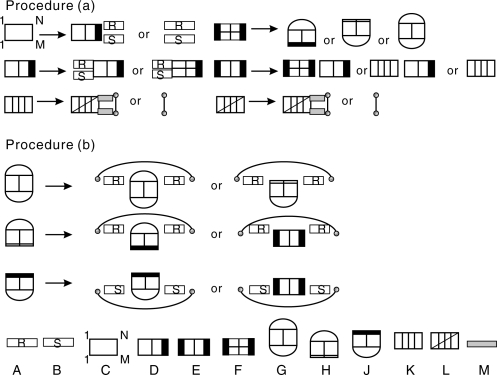
In the following, we redesign the grammar outlined by Huang et al. (2009) so that it explicitly makes use of hybrids. An efficient solution of the partition function problem for RIP requires an unambiguous context-free grammar with the constraint that the number of break points, i.e. the number of non-terminals in each individual production, is as small as possible. This is achieved by introducing several specific types of joint structures that are described in detail in the following. We call a joint right-tight structure (RTS), J^RT_i,j;r,s in J_i1,j1;r1,s1, if its rightmost block is a J_i1,j1;r1,s1-TS and double-tight structure (DTS), J^DT_i,j;r,s in J_i1,j1;r1,s1, if both of its leftmost and rightmost blocks are J_i1,j1;r1,s1-TS's. We remark that this definition is a bit different from the notion of the DTS defined in Huang et al. (2009). In particular, we consider single interaction arcs as particular DTS. Adopting the point of view of Algebraic Dynamic Programming (Giegerich and Meyer, 2002), we regard each decomposition rule as a production in a suitable grammar. Fig. 4 summarizes the three basic steps of the hybrid grammar: (I) “interior arc-removal” to reduce TS. The scheme is complemented by the usual loop decomposition of secondary structures, and (II) “block-decomposition” to split a joint structure into two smaller blocks.

Fig. 4.

Illustration of the reduction of arbitrary joint structures and of right-tight structures, Procedure (a), and of tight structures, Procedure (b). In the bottom row the symbols for the 10 distinct types of structural components are listed: A, B maximal secondary structure segments R[i, j], S[r, s]; C arbitrary joint structure J_1,N;1,M; D right-tight structures J^RT_i,j;r,s; E double-tight structure J^DT_i,j;r,s; F tight structure of type ▽, △ or □; G type □ tight structure J^□_i,j;r,s; H type ▽ tight structure J^▽_i,j;r,s; J type △ tight structure J^△_i,j;r,s; K hybrid structure J^Hy_i,j;h,ℓ; L substructure of a hybrid J^h_i,j;h,ℓ such that R_iS_j and R_hS_ℓ are exterior arcs and J^h_i,j;h,ℓ itself is not a hybrid since it is not maximal; M isolated segment R[i, j] or S[h, ℓ].

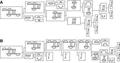
The grammar in Fig. 4 corresponds to the decomposition (parsing) of a joint structure into interior arcs and hybrids. Fig. 5A shows the corresponding parse tree. The full details of the decomposition procedures are described in Section 2 of the Supplementary Material, where we show that for each joint structure J_1,N;1,M, we indeed obtain a unique decomposition tree (parse tree), denoted by T_J1,N;1,M. More precisely, T_J1,N;1,M has root J_1,N;1,M and all other vertices correspond to a specific substructure of J_1,N;1,M obtained by the successive application of the decomposition steps of Fig. 4 and the loop decomposition of the secondary structures. Thus, the hybrid grammar is unambiguous. The two panels of Fig. 5 contrast the grammars of rip1 (Huang et al., 2009) and the hybrid grammar of rip2 introduced here. In rip1, hybrids were immediately decomposed into individual external base pairs and their associated interior loops, so that individual hybrids were not tractable in a straightforward manner.

Fig. 5.

Different grammars lead to different (parse) trees. We show the parse tree T_J1,11;1,11 for the same joint structure J_1,11;1,11 according to the grammars of rip2 (A) and rip1 (B), respectively.

Let us now have a closer look at the energy evaluation of J_i,j;h,ℓ. Each decomposition step in Fig. 4 results in substructures whose energies are assumed to contribute additively and generalized loops that can be evaluated directly. There are the following two basic scenarios:

(I) Interior Arc removal: the first type of decomposition is derived from the decomposition of TS of Huang et al. (2009). Most of the decomposition operations in Procedure (b) displayed in Fig. 4 can be viewed as the “removal” of an arc (corresponding to the closing pair of a loop in secondary structure folding) followed by decomposition. Both, loop type as well as the subsequent decomposition steps depend on the newly exposed structural elements. Following the approach of Zuker and Sankoff (1984) for secondary structures, we treat the loop-decomposition problem by introducing additional matrices. Without loss of generality, we can assume that we open an interior base pair R_iR_j.

The set of base pairs on R[i, j] consists of all interior pairs R_pR_q with i ≤p <q ≤j and all exterior pairs R_p S_h with i ≤ p ≤ j. An interior arc is exposed on R[i + 1, j − 1] if and only if it is not enclosed by any interior arc in R[i, j]. An exterior arc is exposed on R[i + 1, j − 1] if and only if it is not a descendant of any interior arc in R[i + 1, j − 1]. Given R_iR_j, the arcs exposed on R[i + 1, j − 1] correspond to the base pairs immediately interior of R_iR_j. Let us write for this set of ‘exposed base pairs’ and its subsets of interior and exterior arcs. As in secondary structure folding, the loop type is determined by E_R[i,j]≔E_R as follows: E_R = ∅, hairpin loop; E_R = Eⁱ_R and |E_R| = 1, interior loop (including bulge and stacks); E_R = Eⁱ_R, |E_R|≥2, multi-branch loop; E_R = E^e_R, kissing-hairpin loop; |Eⁱ_R|, |E^e_R| ≥ 1, general kissing loop.

This picture needs to be refined even further since the arc removal is coupled with further decomposition of the interval R[i + 1, j − 1]. This prompts us to distinguish TS and DTS with different classes of exposed base pairs on one or both strands. It will be convenient, furthermore, to include information on the type of loop in which it was found.

A TS J^▽_i,j;h,ℓ is of type E, if S[h, ℓ] is not enclosed in any base pair (J^▽,E_i,j;h,ℓ). Suppose J^▽_i,j;h,ℓ is located immediately interior to the closing pair S_pS_q (p < h < ℓ < q). If the loop closed by S_pS_q is a multi-loop, then J^▽_i,j;h,ℓ is of type M (J^▽,M_i,j;h,ℓ). If S_pS_q is contained in a kissing loop, we distinguish the types F and K, depending on whether or not E^e_S[h,ℓ] = ∅.

Analogously, there are in total four types of a hybrid J^Hy_i,j;h,ℓ, i.e. {J^Hy,EE_i,j;h,ℓ, J^Hy,EK_i,j;h,ℓ, J^Hy,KE_i,j;h,ℓ, J^Hy,KK_i,j;h,ℓ}.

(II) Block decomposition: the second type of decomposition is the splitting of joint structures into ‘blocks’. Here, the hybrid grammar differs from the grammar of Huang et al. (2009) in two ways. First, we use the hybrid as a new block of the grammar, decomposing a hybrid by removing its exterior arcs in parallel simultaneously starting from the right. Second, we split a joint structure into blocks via alternating decompositions of RTS and DTS as shown in the Procedure (a) of Fig. 4.

In order to guarantee the maximality hybrids, we observe that the RTS's J^RT,KK_i,j;h,ℓ, J^RT,KE_i,j;h,ℓ, J^RT,EK_i,j;h,ℓ and J^RT,EE_i,j;h,ℓ can appear in two scenarios, depending on whether or not there exists an exterior arc R_i1 S_h1 such that R[i, i₁ − 1] and S[h, h₁ − 1] are isolated segments. In case such an exterior arc exists, we say the RTS is of type (B) or (A), otherwise. Similarly, a DTS, J^DT,KK_i,j;h,ℓ, J^DT,KE_i,j;h,ℓ, J^DT,EK_i,j;h,ℓ or J^DT,EE_i,j;h,ℓ is of type (B) or (A) depending on whether R_iS_h is an exterior arc. In Fig. 6A, we display the decomposition of J^DT,KKB_i,j;h,ℓ into hybrids and RTS of type (A) and in Fig. 6B, we display the decomposition of J^RT,KKA_i,j;h,ℓ into secondary structure segments and DTS accordingly.

Fig. 7.

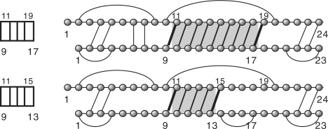
Hybrid probability: the maximality of hybrids implies that—although the intervals [h₁, ℓ₁] and [h₂, ℓ₂] overlap—they belong to two distinct hybrids (gray).

Fig. 6.

Decomposition of J^DT,KKB_i,j;h,ℓ (l.h.s.) and J^RT,KKA_i,j;h,ℓ (r.hs.).

Suppose J^DT_i,j;r,ℓ is a DTS contained in a kissing loop, that is, we have either E^e_R[i,j] ≠ ∅ or E^e_S[h,ℓ] ≠ ∅. Without loss of generality, we may assume E^e_R[i,j] ≠ ∅. Then, at least one of the two ‘blocks’ contains at least an exterior arc belonging to E^e_R[i,j] labeled by K or F, otherwise, see Fig. 6A.

2.3 Forward recursions

The computation of the partition function proceeds ‘from the inside to the outside’, see Equation (3). The recursions are initialized with the energies of individual external base pairs and empty secondary structures on subsequences of length up to 4. In order to differentiate multi- and kissing-loop contributions, we introduce the partition functions Qmi,j and Qki,j. Here, Qmi,j denotes the partition function of secondary structures on R[i, j] or S[i, j] having at least one arc contained in a multi-loop. Similarly, Qki,j denotes the partition function of secondary structures on R[i, j] or S[i, j] in which at least one arc is contained in a kissing loop. Let 𝕁ξ,Y1Y2Y3i,j;h,ℓ be the set of substructures Ji,j;h,ℓ ⊂ J1,N;1,M, induced from some joint structure J1,N;1,M, such that Ji,j;h,ℓ appears in TJ1,N;1,M as an interaction structure of type ξ ∈ {DT, RT, ▽, △, □, ○} with loop-subtypes Y1,Y2 ∈ {M, K, F} on the subintervals R[i, j] and S[h, ℓ], Y3 ∈ {A, B}. Let Qξ,Y1Y2Y3i,j;h,ℓ denote the partition function of the set 𝕁ξ,Y1Y2Y3i,j;h,ℓ. All recursions for Qξ,Y1Y2Y3i,j;h,ℓ represent a reformulation of the hybrid grammar specified in Fig. 4.

For instance, the recursion for Q^DT,KKB_i,j;h,ℓ displayed in Fig. 6A is given by:

(1)

where the corresponding recursion for Q^Hy,KK_i,j;h,ℓ is

(2)

Analogously, the recursions for Q^Hy,EE_i,j;h,ℓ, Q^Hy,EK_i,j;h,ℓ and Q^Hy,KE_i,j;h,ℓ read:

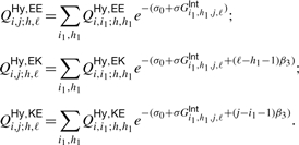(3)

2.4 Hybrid probabilities

Since the probabilities of individual base pairs are not independent, it is not possible to compute the probabilities for particular hybrids directly from them. Hybrid probabilities thus cannot be obtained in a simple way from the backward recursions described by Huang et al. (2009).

Given two RNA sequences, our notion of probability is based on the ensemble of all possible joint interaction structures. Let Q^I denote the partition function of all these joint structures that can formed by two input RNA sequences. The probability of a fixed joint structure J_1,N;1,M is given by

(4)

In difference to the computation of the hybrid-partition function ‘from the inside to the outside’ (IO), the computation of probabilities of specific substructures is obtained ‘from the outside to the inside’. The same principle applies to the computation of base pairing computation of base pairing probabilities of secondary structures (McCaskill, 1990) and joint structures (Huang et al., 2009).

Let J = J_1,N;1,M, with associated decomposition tree T(J) and let Λ_Ji,j;h,ℓ = {J ∣ J_i,j;h,ℓ ∈ T(J)} denote the set of all joint structures J such that J_i,j;h,ℓ is contained in the decomposition tree T(J). Then we have, by construction,

(5)

Following the (OI)-paradigm, the probability of a parent structure, ℙ_θs, is computed prior to the calculation of ℙ_Ji,j;h,ℓ. The conditional probability ℙ_{Ji,j;h,ℓ|θs} equals Q_θs(J_i,j;h,ℓ)/Q(θ_s), where Q(θ_s) is the partition function of θ_s, and Q_θs(J_i,j;h,ℓ) the partition function of all those θ_s, that have in addition J_i,j;h,ℓ as a child in their parse trees. Consequently, ℙ_Ji,j;h,ℓ can inductively be computed by summing over all probabilities ℙ_θs, i.e.

(6)

Let ℙ^Hy_i,j;h,ℓ denote the probability of the set of substructures J such that the specific hybrid substructure, J^Hy_i,j;h,ℓ, appears in the decomposition tree T(J), i.e. J^Hy_i,j;h,ℓ ∈ T(J). Since each joint structure J^Hy_i,j;h,ℓ is either one of the four types J^Hy,EE_i,j;h,ℓ, J^Hy,EK_i,j;h,ℓ, J^Hy,KE_i,j;h,ℓ or J^Hy,KK_i,j;h,ℓ, we arrive at

(7)

We remark that, by construction, for [h₁, ℓ₁]≠[h₂, ℓ₂], the hybrid probabilities ℙ^Hy_i,j;h1,ℓ1 and ℙ^Hy_i,j;h2,ℓ2 quantify disjoint classes of joint structures. This is a consequence of the maximality of hybrids, which implies that, for fixed interval [i, j], each [h₁, ℓ₁] corresponds to a unique hybrid J^Hy_i,j;h1,ℓ1. Based on the notion of hybrid probability, we can introduce

(8)

which is, according to the above, the probability of the target site [i, j] and furthermore

(9)

measuring, for each base i in R the probability that i is contained in a hybrid. A particulary instructive observable is the interaction base pairing matrix, given by

(10)

Clearly, π_i,k measures the probability that a pair of nucleotides (i, k), located on different strands, is contained in an interaction region. In contrast with the base pairing probabilities, large values of π_i,k do not imply that i and k actually form an exterior base pair. Instead, it highlights regions of intermolecular interactions.

2.5 Boltzmann sampling

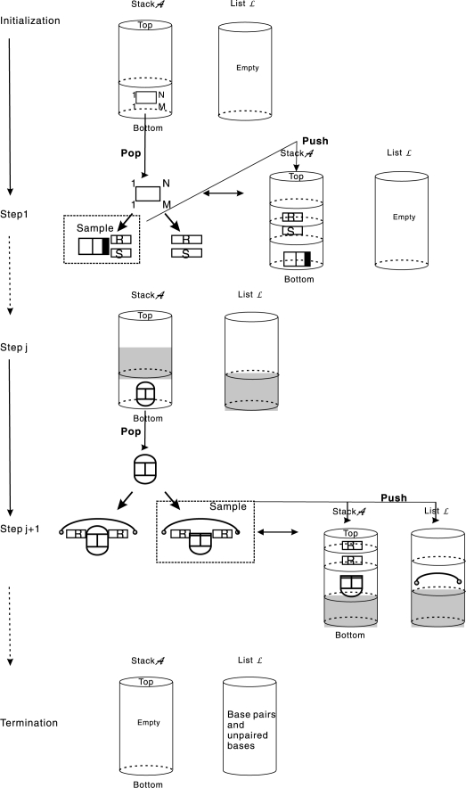
A dynamic programming scheme for the computation of a partition function implies a corresponding stochastic backtracing procedure that can be used to sample from the associated distribution (Tacker et al., 1996). The usefulness of this approach for RNA secondary structures is discussed by Ding and Lawrence (2003). The same ideas can of course also produce representative samples from the Boltzmann equilibrium distribution of RNA interaction structures (Fig. 8).

Fig. 8.

Stochastic backtracing algorithm: elements of stack 𝒜 are successively decomposed according to the hybrid-grammar. The resulting arcs and unpaired vertices are stored in the list ℒ which, once 𝒜 is empty, eventually contains the Boltzmann-sampled interaction structure.

The basic data structure of the algorithm is a stack 𝒜 that stores tuples of the form {(i, j; h, ℓ; ξ)} describing a pair of intervals [i, j] in R and [h, ℓ] in S and the type ξ of the—not further specified—joint structure formed by the two intervals. The stack 𝒜, initialized with (1, N; 1, M, ?) where ‘?’ denotes the unspecified type, guides the backtracing which is complete as soon as 𝒜 is empty. A list ℒ is used to collect the interior and exterior arcs and unpaired bases generated by the decompositions and eventually define the sampled interaction structure. In the first step, (1, N; 1, M, ?) is decomposed according to the grammar in Fig. 4 into either (i) a pair of secondary structures, or (ii) a RTS (i, N; j, M; RTEE) with probabilities derived as explained above. Depending on the stochastic choice, we push either (i) (1, N; 0, 0; sec) and (0, 0; 1, M; sec) or (ii) (1, i − 1; 0, 0, sec), (0, 0; 1, j − 1; sec) and (i, N; j, M; RTEE) into the stack 𝒜.

Given 𝒜 and ℒ, we can associate a probability by considering the decomposition of the particular type of joint structure. For instance, suppose we have extracted (i, j; h, ℓ, DTKKB) from stack 𝒜, see Fig. 6. Then, the probabilities for continuing with one of the five decompositions displayed in Fig. 6, for each position of the break points i₁ ∈ [i, j] and h₁ ∈ [h, ℓ], is given by

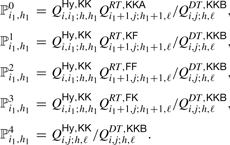One of these decompositions is accordingly sampled and the respective output is pushed back into stack 𝒜. For instance, if ℙ¹_i1,h1 is selected, then we push (i, i₁; h, h₁; HyKK) and (i₁ + 1, j; h₁ + 1, ℓ; RTKF) back into stack 𝒜.

3 RESULTS AND CONCLUSIONS

We presented here a modified and improved unambiguous grammar for the RIP. Compared with rip1 (Huang et al., 2009), it reduces the computational efforts, in particular the memory consumption, by about a third. In the Supplementary Material, we contrast rip2 with rip1 and show that hybrids (as opposed to TS, RTS or DTS) are uniquely suited for identifying the interaction regions of two RNA molecules. The complete set of recursions is compiled in Section 3 of the Supplementary Material. It comprises 9 4D-arrays Q^△,▽,□_i,j;r,s for TS of various types, 20 4D-arrays Q^RT_i,j;r,s for RTS and 20 4D-arrays Q^DT_i,j;r,s for DTS. The implementation has been complemented by a stochastic backtracing facility. Fig. 9 gives an example of the output produced by rip2 (see also Supplementary Material, Fig. 4). Despite algorithmic improvements, rip2 still requires quite substantial computational resources for practical applications. rip2 is in practise limited to problem sizes of on current hardware. While rip2 is still not an efficient tool for large-scale routine applications, it is suitable for investigating the fine details of particular interactions. Future work will thus focus on controlled approximations with the aim of a drastic reduction of both: CPU and memory consumption.

Fig. 9.

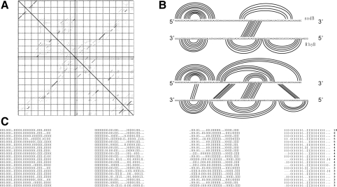
Interaction of sodB–RhyB. (A) Base-pairing probability matrix. The upper right triangle shows the probabilities obtained from the exact backwards recursion, the lower left triangle is the estimate from a sample of 10 000 structures obtained by stochastic backtracing, showing that the estimates converge quickly. (B) Comparison of the structure proposed in Geissmann and Touati (2004) and the rip2 prediction. While the major stable hairpins agree and rip2 correctly predicts the primary interaction region, rip2 also identifies additional interaction regions that may stabilize the interaction. (C) Sampled joint structures (here the 20 most frequent ones) are represented as dot-bracket strings: () and [] represent pairs of interior and exterior arc, respectively, while dots indicate unpaired bases. | separates the two RNA sequences which are both written in 5^′ → 3^′ direction.

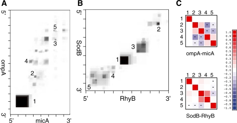
The major advantage of stochastic sampling is that it provides a generic and convenient means to estimate quantities that cannot be easily computed directly by backwards recursion (Ding and Lawrence, 2003). Both, the ompA-MicA and sodB-RhyB complexes show a primary, highly likely, hybrid region and several additional less stable points of contact, see Fig. 10. In these examples, it is of interest to investigate in detail how the putative interaction regions influence each other: is the binding cooperative so that the major hybrids in Fig. 10 are positively correlated, or do they constitute mutually exclusive contacts? Once a sufficiently large Boltzmann sample is obtained, we can easily compute, e.g. correlations ρ_PQ between indicator variables P and Q that measure the existence of external base pairs in two different hybrids. Fig. 10C provide examples, showing that there are strong correlations between hybridization regions. These multiple contacts can contribute substantially to the total interaction energy.

Fig. 10.

Interaction maps. The ompA–MicA interaction (A) has a dominating interaction region that brings together the 3^′ end of ompA and the 5^′ terminus of MicA. The sodB–RhyB interactions (B) has two clear hybridization regions in the middle of the molecules and a diffuse contact area at the 3^′ end of sodB. The grayscale show the probabilities π_ik. Tick marks indicate every 10th nucleotide. The correlations between the major binding regions can be computed easily from Boltzmann samples. The heatmaps show the correlation coefficients for the most probable interaction regions (indicated by numbers in the interaction maps). (C) For sodB–RhyB, we observe fairly weak correlations, except for the cooperative interaction between contacts 3 and 4. In case of ompA–MicA, we observe strong negative correlations between conflicting hybridization regions.

REFERENCES

- Akutsu T. Dynamic programming algorithms for RNA secondary structure prediction with pseudoknots. Disc. Appl. Math. 2000;104:45–62. [Google Scholar]
- Alkan C, et al. RNA-RNA interaction prediction and antisense RNA target search. J. Comput. Biol. 2006;13:267–282. doi: 10.1089/cmb.2006.13.267. [DOI] [PubMed] [Google Scholar]
- Andronescu M, et al. Secondary structure prediction of interacting RNA molecules. J. Mol. Biol. 2005;345:1101–1112. doi: 10.1016/j.jmb.2004.10.082. [DOI] [PubMed] [Google Scholar]
- Argaman L, Altuvia S. fhlA repression by OxyS RNA: kissing complex formation at two sites results in a stable antisense-target RNA complex. J. Mol. Biol. 2000;300:1101–1112. doi: 10.1006/jmbi.2000.3942. [DOI] [PubMed] [Google Scholar]
- Bachellerie J, et al. The expanding snoRNA world. Biochimie. 2002;84:775–790. doi: 10.1016/s0300-9084(02)01402-5. [DOI] [PubMed] [Google Scholar]
- Banerjee D, Slack F. Control of developmental timing by small temporal RNAs: a paradigm for RNA-mediated regulation of gene expression. Bioessays. 2002;24:119–129. doi: 10.1002/bies.10046. [DOI] [PubMed] [Google Scholar]
- Benne R. RNA editing in trypanosomes. the use of guide RNAs. Mol. Biol. Rep. 1992;16:217–227. doi: 10.1007/BF00419661. [DOI] [PubMed] [Google Scholar]
- Bernhart S, et al. Partition function and base pairing probabilities of RNA heterodimers. Algorithms Mol. Biol. 2006;1:3. doi: 10.1186/1748-7188-1-3. [DOI] [PMC free article] [PubMed] [Google Scholar]
- Busch A, et al. IntaRNA: efficient prediction of bacterial sRNA targets incorporating target site accessibility and seed regions. Bioinformatics. 2008;24:2849–2856. doi: 10.1093/bioinformatics/btn544. [DOI] [PMC free article] [PubMed] [Google Scholar]
- Chitsaz H, et al. Proceedings of the 9th Workshop on Algorithms in Bioinformatics (WABI) Vol. 5724. Lectures Notes in Computer Science. Springer; 2009a. biRNA: fast RNA-RNA binding sites prediction; pp. 25–36. [Google Scholar]
- Chitsaz H, et al. A partition function algorithm for interacting nucleic acid strands. Bioinformatics. 2009b;25:i365–i373. doi: 10.1093/bioinformatics/btp212. [DOI] [PMC free article] [PubMed] [Google Scholar]
- Ding Y, Lawrence CE. A statistical sampling algorithm for RNA secondary structure prediction. Nucleic Acid Res. 2003;31:7280–7301. doi: 10.1093/nar/gkg938. [DOI] [PMC free article] [PubMed] [Google Scholar]
- Dirks R, et al. Thermodynamic analysis of interacting nucleic acid strands. SIAM Rev. 2007;49:65–88. [Google Scholar]
- Dowell RD, Eddy SR. Evaluation of several lightweight stochastic context-free grammars for RNA secondary structure prediction. BMC Bioinformatics. 2004;5:7. doi: 10.1186/1471-2105-5-71. [DOI] [PMC free article] [PubMed] [Google Scholar]
- Geissmann T, Touati D. Hfq, a new chaperoning role: binding to messenger RNA determines access for small RNA regulator. EMBO J. 2004;23:396–405. doi: 10.1038/sj.emboj.7600058. [DOI] [PMC free article] [PubMed] [Google Scholar]
- Giegerich R, Meyer C. Lecture Notes in Computer Science. Vol. 2422. London: Springer; 2002. Algebraic Dynamic Programming; pp. 349–364. [Google Scholar]
- Hekimoglu B, Ringrose L. Non-coding RNAs in polycomb/trithorax regulation. RNA Biol. 2009;6:129–137. doi: 10.4161/rna.6.2.8178. [DOI] [PubMed] [Google Scholar]
- Hofacker IL, et al. Fast folding and comparison of RNA secondary structures. Monatsh. Chem. 1994;125:167–188. [Google Scholar]
- Huang FWD, et al. Partition function and base pairing probabilities for RNA-RNA interaction prediction. Bioinformatics. 2009;25:2646–2654. doi: 10.1093/bioinformatics/btp481. [DOI] [PubMed] [Google Scholar]
- Kugel J, Goodrich J. An RNA transcriptional regulator templates its own regulatory RNA. Nat. Struct. Mol. Biol. 2007;3:89–90. doi: 10.1038/nchembio0207-89. [DOI] [PubMed] [Google Scholar]
- McCaskill JS. The equilibrium partition function and base pair binding probabilities for RNA secondary structure. Biopolymers. 1990;29:1105–1119. doi: 10.1002/bip.360290621. [DOI] [PubMed] [Google Scholar]
- McManus MT, Sharp PA. Gene silencing in mammals by small interfering RNAs. Nat. Rev. 2002;3:737–747. doi: 10.1038/nrg908. [DOI] [PubMed] [Google Scholar]
- Mneimneh S. On the approximation of optimal structures for RNA-RNA interaction. IEEE/ACM Trans. Comp. Biol. Bioinform. 2009;6:682–688. doi: 10.1109/TCBB.2007.70258. [DOI] [PubMed] [Google Scholar]
- Mückstein U, et al. Thermodynamics of RNA-RNA binding. Bioinformatics. 2006;22:1177–1182. doi: 10.1093/bioinformatics/btl024. [DOI] [PubMed] [Google Scholar]
- Mückstein U, et al. Translational control by RNA-RNA interaction: improved computation of RNA-RNA binding thermodynamics. In: Elloumi M, et al., editors. Bioinformatics Research and Development — BIRD 2008. Vol. 13. Berlin: Communication in Computer and Information Science. Springer; 2008. pp. 114–127. [Google Scholar]
- Narberhaus F, Vogel J. Sensory and regulatory RNAs in prokaryotes: A new german research focus. RNA Biol. 2007;4:160–164. doi: 10.4161/rna.4.3.5308. [DOI] [PubMed] [Google Scholar]
- Pervouchine D. IRIS: intermolecular RNA interaction search. Proc. Genome Inform. 2004;15:92–101. [PubMed] [Google Scholar]
- Qin J, Reidys CM. A combinatorial framework for RNA tertiary interaction. Technical Report 0710.3523, arXiv. 2007 Available at http://arxiv.org/PS_cache/arxiv/pdf/0710/0710.3523v3.pdf. [Google Scholar]
- Rehmsmeier M, et al. Fast and effective prediction of microRNA/target duplexes. Gene. 2004;10:1507–1517. doi: 10.1261/rna.5248604. [DOI] [PMC free article] [PubMed] [Google Scholar]
- Rivas E, Eddy SR. A dynamic programming algorithms for RNA structure prediction including pseudoknots. J. Mol. Biol. 1999;285:2053–2068. doi: 10.1006/jmbi.1998.2436. [DOI] [PubMed] [Google Scholar]
- Salari R, et al. Proceedings of the 9th Workshop on Algorithms in Bioinformatics (WABI) Vol. 5724. Lecture Notes in Computer Science. Springer; 2009. Fast prediction of RNA-RNA interaction; pp. 261–272. [Google Scholar]
- Tacker M, et al. Algorithm independent properties of RNA structure prediction. Eur. Biophy. J. 1996;25:115–130. [Google Scholar]
- Tafer H, et al. RNAsnoop: efficient target prediction for box H/ACA snoRNAs. Bioinformatics. 2009 doi: 10.1093/bioinformatics/btp680. University of Leipzig. Available at http://www.bioinf.uni-leipzig.de/Publications/PREPRINTS/09-025.pdf. [DOI] [PubMed] [Google Scholar]
- Tjaden B, et al. Target prediction for small, noncoding RNAs in bacteria. Nucleic Acids Res. 2006;34:2791–2802. doi: 10.1093/nar/gkl356. [DOI] [PMC free article] [PubMed] [Google Scholar]
- Udekwu K, et al. Hfq-dependent regulation of OmpA synthesis is mediated by an antisense RNA. Genes Dev. 2005;19:2355–2366. doi: 10.1101/gad.354405. [DOI] [PMC free article] [PubMed] [Google Scholar]
- Urban JH, Vogel J. Translational control and target recognition by Escherichia coli small RNAs in vivo. Nucleic Acids Res. 2007;35:1018–1037. doi: 10.1093/nar/gkl1040. [DOI] [PMC free article] [PubMed] [Google Scholar]
- Zuker M, Sankoff D. RNA secondary structures and their prediction. Bull. Math. Biol. 1984;46:591–621. [Google Scholar]
Associated Data
This section collects any data citations, data availability statements, or supplementary materials included in this article.