Optimized motion estimation for MRE data with reduced motion encodes

Abstract

Motion estimation is an essential step common to all magnetic resonance elastography (MRE) methods. For dynamic techniques, the motion is obtained from a sinusoidal fit of the image phase at multiple, uniformly spaced relative phase offsets, φ, between the motion and the motion encoding gradients (MEGs). Generally, eight values of φ sampled at the Nyquist interval π/4 over [0, 2π). We introduce a method, termed reduced motion encoding (RME), that reduces the number of φ required, thereby reducing the imaging time for an MRE acquisition. A frequency-domain algorithm was implemented using the discrete Fourier transform (DFT) to derive the general least-squares solution for the motion amplitude and phase given an arbitrary number of φ. A closed form representation of the condition number of the transformation matrix which is used for estimating motion was introduced to determine the sensitivity to noise for different sampling patterns of φ. Simulation results confirmed the minimum error sampling patterns suggested from the condition number maps. The minimum noise in the motion estimate is obtained when the sampled φ are essentially evenly distributed over the range [0, π) with an interval π/n, where n is the number of φ sampled, or alternatively with an interval 2π/n over the range [0, 2π) which represents the Nyquist interval. Simulations also show that the noise level decreases as n increases as expected. The decrease in noise is the largest when n is small and it becomes less significant as n increases. The algorithm also makes it possible to estimate the motion from only two values of φ, which cannot be accomplished with traditional methods because sampling at the Nyquist interval is indeterminate. Finally, noise levels in motion estimated from phantom studies and in vivo results taken with different n agreed with that predicted by simulation and condition number calculations.

1. Introduction

Magnetic resonance elastography (MRE) measures and visualizes the mechanical properties of a tissue in vivo. Different approaches have been described based on dynamic methods (Muthupillai et al 1995, Kruse et al 2000, Suga et al 2003) and steady-state techniques (Sinkus et al 2000, Weaver et al 2001, McCracken et al 2005). Dynamic MRE applies intermittent or continuous harmonic mechanical excitation to the tissue and estimates the shear modulus from the measured wavelength. Generally boundary effects create reflections that interfere with the induced wavefront which can confound the wavelength estimation involved in determining the mechanical properties of the tissue. While in complex organs such as the breast, the accurate quantification of wavelength is difficult. Manduca et al (1996) circumvented this limitation by applying the local frequency estimation (LFE) to MRE data. Recently, a novel transient method was developed as an alternative (McCracken et al 2005). This approach uses transient impulses for mechanical excitation instead of harmonic wavefronts and exhibited better contrast resolution of deeper brain tissues. In the steady-state methods, any vibration pattern is perfectly acceptable but the boundary effects must be incorporated into the mechanical property estimation process.

For dynamic and steady-state MRE methods, two steps are required to obtain a map of tissue mechanical properties. The first step is to estimate the induced tissue motion using a phase contrast pulse sequence (Muthupillai et al 1996, Sinkus et al 2000, Weaver et al 2001). The sequence is modified to characterize cyclic motion that uses multiple acquisitions at different relative phases between the motion and motion encoding gradients. Then in the second step the tissue motion information is used to reconstruct the tissue mechanical properties.

A number of approaches have been developed to reduce acquisition time without introducing significant additional noise. For example, Hadamard encoding of motion in 3D can reduce the imaging time by 33% (Hausmann et al 1991). It effectively uses one acquisition as the reference for all three-acquisition directions and therefore reduces the conventional six-acquisition method to a four-acquisition scheme. In another approach, Weaver et al (2003) used a frequency encoding gradient to encode both periodic motion and position to increase image SNR and reduce image acquisition time. In this paper, we present a motion reconstruction method which reduces the acquisition time by minimizing the number of relative phases that are required for the reconstruction. A frequency-domain least-squares optimization model was developed to estimate the motion using an arbitrary number and distribution of relative phases. Strictly speaking, the method is not a nonuniform Fourier transform algorithm. Most nonuniform Fourier transforms are based on interpolating on an over-sampled FFT for randomly spaced data (Dutt and Rokhlin 1993, Liu and Nguyen, 1998, Beylkin, 1995, Steidl, 1998). Our method is a least-squares algorithm fitting the designated nonequispaced samples to a known-frequency harmonic wave. The nonequispaced samples are selected based on smaller-unit equispaced samples; thus we can derive an exact form representation for the motion parameters.

A general form was developed to estimate motion with any number of phase offsets, in comparison with the conventional method where the number of phase offsets is restricted to powers of 2 greater than or equal to 4. In a clinical examination, if the recovered motion using four acquisitions is too noisy, six or seven phases might be sufficient without acquiring eight phase offsets. The flexibility to reconstruct the motion from arbitrarily sampled phases allows more flexibility in the acquisition; e.g., the motion might be reconstructed dynamically during the acquisition and halted when a specified SNR is achieved. The method also makes it possible to reconstruct the motion with two phase offsets, which is lower than the limit of four phase offsets required by the conventional method. Although algorithm such as three-point discrete Fourier transform (DFT) for fast generalized Fourier analysis has been applied by many groups (Dubois and Venetsanopoulos 1978, Suzuki et al 1986), none have previously applied this to MRE. In addition reconstructing the motion from a smaller set of sampled phases might be useful in reducing the acquisition time to image physiologic motion more rapidly.

2. Methods

The phase of each pixel in the MR image, f (φ), can be expressed as a function of the relative phase offset φ (Muthupillai et al 1995, 1996):

$$f(\phi )=Acos(\phi +\theta ),$$ (1)

where φ is the relative phase offset between the externally induced motion and motion encoding gradients. The amplitude, A, and phase, θ, characterize the harmonic motion completely and can be used to recover the mechanical properties with different reconstruction techniques, such as direct substitution of image displacement into the elasticity equations (Manduca et al 2001) or subzone-based inversion (Van Houten et al 1999).

The estimation method used previously was the FFT, which transforms the measured image phase from the φ domain to a frequency domain (Oppenheim et al 1999). However, this method requires φ to be sampled evenly across one cycle of the motion at the Nyquist intervals, φ = 2π φ_n/N (φ_n = 0,…, N − 1) where N is the number of φ acquired. Besides, N must be a power of 2, since the FFT requires dyadic sampling. We present here a detailed procedure for fitting the image phase with the cosine function in the frequency domain for arbitrary sampling distributions of φ. The method eliminates the dyadic sampling requirements and provides the flexibility to optimize the number of measured relative phases and the resulting SNR. In addition, this method provides a way to process incomplete data sets in situations where physiologic activity restricts imaging times, such as heart data.

2.1. The least-squares fitting with full acquisition

Harmonic motion of a known frequency is completely characterized by the amplitude, A, and relative phase, θ. Generally the motion information is estimated by a least-squares fit in the frequency domain when transforming the time-domain image phases into the frequency domain. Because the frequencies of the motion and of the motion encoding gradient are controlled very accurately, for linear elastic materials, the desired signal energy of the DFT of the image phases is concentrated exclusively in the second term, i.e., in the fundamental frequency (Oppenheim et al 1999).

We will first examine the process for uniformly spaced samples in detail. The cosine function, f(φ_n), can be expressed as a linear combination of complex exponentials:

$$f({\phi }_n)=Acos\left(\frac{2\pi {\phi }_n}{N}+\theta \right)=\frac{A}{2}{\text{e}}^{\text{i}(\frac{2\pi {\phi }_n}{N}+\theta )}+\frac{A}{2}{\text{e}}^{-\text{i}(\frac{2\pi {\phi }_n}{N}+\theta )}.$$ (2)

The corresponding discrete frequency-domain sequence F(0), F(1),…, F(N − 1) is obtained by applying the DFT on the right-hand side of equation (2) (Oppenheim et al 1999).

Explicitly

$$\begin{array}{ll}F({\omega }_n)& =\sum _{{\phi }_n=0}^{N-1}f({\phi }_n){\text{e}}^{-\text{i}2\pi {\phi }_n{\omega }_n/N}\\ & =\sum _{{\phi }_n=0}^{N-1}\frac{A}{2}{\text{e}}^{\text{i}(\frac{2\pi {\phi }_n}{N}+\theta )}{\text{e}}^{-\text{i}2\pi {\phi }_n{\omega }_n/N}+\sum _{{\phi }_n=0}^{N-1}\frac{A}{2}{\text{e}}^{-\text{i}(\frac{2\pi {\phi }_n}{N}+\theta )}{\text{e}}^{-\text{i}2\pi {\phi }_n{\omega }_n/N}\\ & =\frac{A}{2}{\text{e}}^{\text{i}\theta }\sum _{{\phi }_n=0}^{N\sum 1}{\text{e}}^{\text{i}\frac{2\pi {\phi }_n}{N}(1-{\omega }_n)}+\frac{A}{2}{\text{e}}^{-\text{i}\theta }\sum _{{\phi }_n=0}^{N-1}{\text{e}}^{-\text{i}\frac{2\pi {\phi }_n}{N}(1+{\omega }_n)}\\ & =\{\begin{array}{cc}0,\hfill & {\omega }_n\ne 1,N-1\hfill \\ \frac{AN}{2}{\text{e}}^{\text{i}\theta },\hfill & {\omega }_n=1\hfill \\ \frac{AN}{2}{\text{e}}^{-\text{i}\theta },\hfill & {\omega }_n=N-1.\hfill \end{array}\end{array}$$ (3)

For a harmonic signal at the fundamental frequency, all terms of F(ω) are zero except the conjugate pair F(1) and F(N − 1), which preserve the information of amplitude A and phase θ. Either of them can be used to estimate A and θ.

2.2. The least-squares fitting with partial phase data

Full acquisition of raw MR phase data, however, can require long acquisition time to obtain all N values. The new method finds the contribution of each time-domain sample to the fundamental frequency and estimates A and θ using fewer values of f(φ_n). From the general expression for F(ω_n)

$$F({\omega }_n)=\frac{A}{2}{\text{e}}^{\text{i}\theta }\sum _{{\phi }_n=0}^{N-1}{\text{e}}^{\text{i}\frac{2\pi {\phi }_n}{N}(1-{\omega }_n)}+\frac{A}{2}{\text{e}}^{-\text{i}\theta }\sum _{{\phi }_n=0}^{N-1}{\text{e}}^{-\text{i}\frac{2\pi {\phi }_n}{N}(1+{\omega }_n)},$$

the fundamental frequency term F(1) may be retrieved by separating the contribution from each time-domain sample:

$$\begin{array}{ll}F(1)& =\frac{A}{2}{\text{e}}^{\text{i}\theta }\sum _{{\phi }_n=0}^{N-1}\text{1}+\frac{A}{2}{\text{e}}^{-\text{i}\theta }\sum _{{\phi }_n=0}^{N-1}{\text{e}}^{-\text{i}\frac{4\pi {\phi }_n}{N}}\\ & =\frac{AN}{2}(cos\theta +isin\theta )+\frac{A}{2}(cos\theta -isin\theta )\\ & \times \left[\left(cos\frac{4\pi {\phi }_{n1}}{N}+cos\frac{4\pi {\phi }_{n2}}{N}+\dots \right)-i\left(sin\frac{4\pi {\phi }_{n1}}{N}+sin\frac{4\pi {\phi }_{n2}}{N}+\dots \right)\right].\end{array}$$ (4)

Different patterns of φ result in different formulations for the fundamental frequency F(1). The matrix form of the real and imaginary parts of F(1) can be derived by applying a transformation matrix, T, on the amplitude and phase matrix, D:

$$F=TD,$$ (5)

where $F=\left(\begin{array}{c}Re[F(1)]\\ Im[F(1)]\end{array}\right),D=\left(\begin{array}{c}\frac{A}{2}cos\theta \\ \frac{A}{2}sin\theta \end{array}\right)$ and T varies with different patterns of φ_n:

$$T=\left[\begin{array}{ll}N+\left(cos\frac{4\pi {\phi }_{n1}}{N}+cos\frac{4\pi {\phi }_{n2}}{N}+\dots \right)& -\left(sin\frac{4\pi {\phi }_{n1}}{N}+sin\frac{4\pi {\phi }_{n2}}{N}+\dots \right)\\ -\left(sin\frac{4\pi {\phi }_{n1}}{N}+sin\frac{4\pi {\phi }_{n2}}{N}+\dots \right)& N-\left(cos\frac{4\pi {\phi }_{n1}}{N}+cos\frac{4\pi {\phi }_{n2}}{N}+\dots \right)\end{array}\right].$$

The D matrix can be computed as T⁻¹F and motion parameters A and θ can then be estimated. At least two relative phases are required except for the case φ_n2 = φ_n1 ± N/2, when φ_n2 and φ_n1 give identical information because of the symmetry about 2π for both sines and cosines in the T matrix. Here is the proof. In the case of different φ_n1 where φ_n1b = φ_n1a + N/2, the T matrix for φ_n1a and φ_n1b can be expressed respectively as

$$\begin{array}{ll}{T}_a& =\left[\begin{array}{ll}N+\left(cos\frac{4\pi {\phi }_{n1a}}{N}+cos\frac{4\pi {\phi }_{n2}}{N}+\dots \right)& -\left(sin\frac{4\pi {\phi }_{n1a}}{N}+sin\frac{4\pi {\phi }_{n2}}{N}+\dots \right)\\ -\left(sin\frac{4\pi {\phi }_{n1a}}{N}+sin\frac{4\pi {\phi }_{n2}}{N}+\dots \right)& N-\left(cos\frac{4\pi {\phi }_{n1a}}{N}+cos\frac{4\pi {\phi }_{n2}}{N}+\dots \right)\end{array}\right],\\ T_b& =\left[\begin{array}{ll}N+\left(cos\frac{4\pi {\phi }_{n1b}}{N}+cos\frac{4\pi {\phi }_{n2}}{N}+\dots \right)& -\left(sin\frac{4\pi {\phi }_{n1b}}{N}+sin\frac{4\pi {\phi }_{n2}}{N}+\dots \right)\\ -\left(sin\frac{4\pi {\phi }_{n1b}}{N}+sin\frac{4\pi {\phi }_{n2}}{N}+\dots \right)& N-\left(cos\frac{4\pi {\phi }_{n1b}}{N}+cos\frac{4\pi {\phi }_{n2}}{N}+\dots \right)\end{array}\right]\\ & =[\begin{array}{l}N+\left(cos\frac{4\pi ({\phi }_{n1a}+N/2)}{N}+cos\frac{4\pi {\phi }_{n2}}{N}+\dots \right)\\ -\left(sin\frac{4\pi ({\phi }_{n1a}+N/2)}{N}+sin\frac{4\pi {\phi }_{n2}}{N}+\dots \right)\end{array}\\ & \begin{array}{l}-\left(sin\frac{4\pi ({\phi }_{n1a}+N/2)}{N}+sin\frac{4\pi {\phi }_{n2}}{N}+\dots \right)\\ N-\left(cos\frac{4\pi ({\phi }_{n1a}+N/2)}{N}+cos\frac{4\pi {\phi }_{n2}}{N}+\dots \right)\end{array}]\\ & =[\begin{array}{l}N+\left(cos\left(\frac{4\pi {\phi }_{n1a}}{N}+2\pi \right)+cos\frac{4\pi {\phi }_{n2}}{N}+\dots \right)\\ -\left(sin\left(\frac{4\pi {\phi }_{n1a}}{N}+2\pi \right)+sin\frac{4\pi {\phi }_{n2}}{N}+\dots \right)\end{array}\\ & \begin{array}{l}-\left(sin\left(\frac{4\pi {\phi }_{n1a}}{N}+2\pi \right)+sin\frac{4\pi {\phi }_{n2}}{N}+\dots \right)\\ N-\left(cos\left(\frac{4\pi {\phi }_{n1a}}{N}+2\pi \right)+cos\frac{4\pi {\phi }_{n2}}{N}+\dots \right)\end{array}]=T_a,\end{array}$$ (6)

which are the same. As a consequence, the range of φ we are interested in can be limited to [0, π].

By selecting different φ_n, the reconstruction process results in different noise levels for A and θ. The optimum combinations were obtained using a closed-form solution for the condition number and are presented in the next section.

2.3. Condition number of partial phase data motion reconstructions

Different combinations of relative phase offsets result in different noise amplifications when calculating the D matrix from F and T in equation (5). The following discussion uses the condition number to evaluate the error propagation from the measured value F to the amplitude and phase matrix, D.

When a small perturbation is applied on F, the problem of computing D = T⁻¹F has the condition number k (Trefethen and Bau 1997, Skare et al 2000):

$$k=\underset{\delta F}{sup}\left(\frac{\Vert T^{-1}\cdot \delta F\Vert }{\Vert \delta F\Vert }/\frac{\Vert T^{-1}F\Vert }{\Vert F\Vert }\right).$$

sup means the supremum of the formula over all infinitesimal perturbations δF. With this definition, k is bounded by

$$k\ge \frac{\Vert T^{-1}\cdot \delta F\Vert }{\Vert \delta F\Vert }/\frac{\Vert T^{-1}F\Vert }{\Vert F\Vert }=\frac{\Vert T^{-1}\cdot \delta F\Vert }{\Vert T^{-1}F\Vert }/\frac{\Vert \delta F\Vert }{\Vert F\Vert }.$$

Then,

$$\frac{\Vert T^{-1}\cdot \delta F\Vert }{\Vert T^{-1}F\Vert }\le k\frac{\Vert \delta F\Vert }{\Vert F\Vert }\Rightarrow \frac{\Vert \delta D\Vert }{\Vert D\Vert }\le k\frac{\Vert \delta F\Vert }{\Vert F\Vert }.$$

The expression indicates that the relative error in D is bounded by the condition number of the matrix T⁻¹ times the relative error in the measurement F. When the condition number is close or equal to 1, the propagated error in D will be close to the error in the measurement F which is the case for an orthogonal matrix T such as that of a Fourier transform with full number of phase offsets employed. On the other hand, a large condition number results in a large error in D because the measurement error is amplified. Thus, by analyzing the condition number of the matrix T (T⁻¹), we can decide which pattern of relative phase offsets minimizes the amplification of noise during the motion estimation process.

3. Simulation results

In addition to the closed form of the condition number, Monte Carlo simulations were used to examine the variation in the noise level with different combinations of relative phases between the motion and the MEGs, φ. Tests on different numbers of φ were performed. The simulation results are also compared with the solution calculated from the condition number. Finally, the optimal sampling patterns for each number of relative phase offsets were selected and the corresponding noise levels were plotted.

3.1. Tests with two relative phases

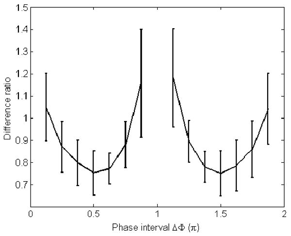
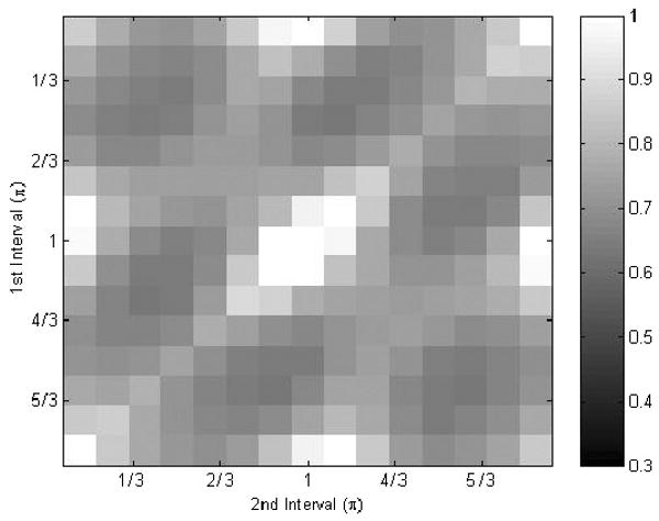
The simulation was first performed with two relative phase offsets, where the conventional method cannot be applied because of the indeterminacy of the solution. Figure 1 shows the influence of the phase interval between the sampled φ on the reconstruction error in A when the MR signal is corrupted by 5% random noise on the magnitude. The mean value of the estimation error is plotted versus the phase interval. Error bars are provided in the cases where the first phase offset is not fixed. Figure 2 shows the corresponding condition number map. From both figures, the trends in the estimation error on the intervals [0, π) and [π, 2π) are found to be similar. The optimal phase intervals for two relative phases can be found around π/2 or 3π/2, while the intervals near the ‘pole’ area 0, π or 2π give very large errors. Similar noise patterns were found when estimating the phase θ and displacement (A* cos θ) of the motion.

Figure 1.

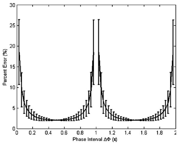
The mean value of estimation error in the motion amplitude, with error bars, as a function of the phase interval where the starting phase offset is not fixed.

Figure 2.

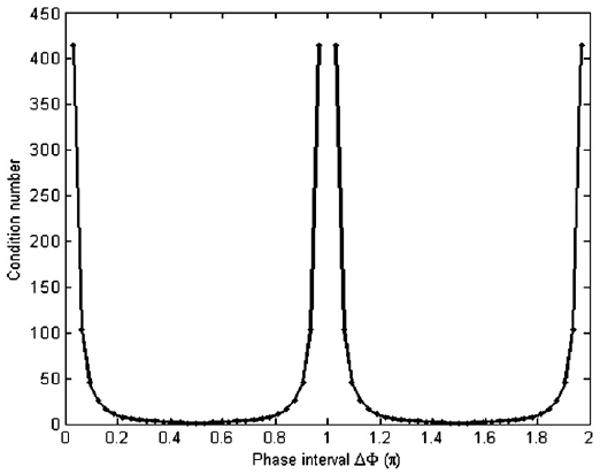
The condition number map of the transformation matrix T⁻¹ for two relative phases.

From equation (6) it is evident that φ_n = φ_n1 and φ_n = φ_n1 + N/2 (i.e. an interval π) have the same T which is why the trends over the [0, π) and [π, 2π) intervals are the same. It also suggests that the estimation could not be applied when the phase intervals are 0, π or 2π. Other than these ‘pole’ areas, a fairly wide range of values generate small errors with little variation. In addition, the equation explains why for two relative phases, the algorithm makes the estimation possible where the conventional reconstruction method cannot be applied using the Nyquist interval φ = π.

Some nonuniform sampling methods (Scoular and Fitzgerald, 1992, Prendergast et al 2004) result in similar sampling patterns as found in our simulation result; however, their sampling rate must be at least the Nyquist rate. This limitation is not applicable in our case because the frequency of the signal is known.

3.2. More than two relative phases

The simulated error patterns from estimating motion parameters using three to five relative phases and the relevant condition number map are illustrated in figures 3(a)–(f), still with 5% random noise (SNR = 20) added to the magnitude of the raw MR data. For three and four phase offset cases, each interval between the adjacent phase offsets is used as the image axis in order to reduce the image dimensions.

Figure 3.

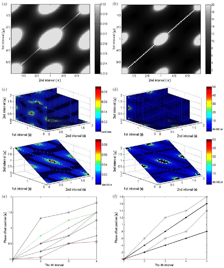
(a) The mean relative error in the estimated displacement (A* cos θ) when three relative phases are used. (b) The condition number map of the transformation matrix T⁻¹. (c) The simulated error patterns of estimating A from four relative phases. (d) The condition number map with characteristic slices for four relative phase offsets. (e) Phase offset position versus the ith phase offset with the condition number = 1 from four relative phases. The relative phases started at a fixed position are plotted. (f) Phase offset position versus the ith phase offset with the condition number = 1 from five relative phases.

(This figure is in colour only in the electronic version)

The error image of figure 3(a) is windowed tightly to show the dark regions where the error is minimized. Several other large bright regions were also found in the noise pattern map. Nine ‘poles’, i.e. the indeterminate points, such as (0, 0) and (π, 2π), were included in these regions and were associated with extremely large errors. Symmetry is found in the four quadrants of this plot. The reconstruction error patterns on A and θ have a similar pattern to that of the displacement and are not shown here. Figure 3(b) is the condition number map of the transformation matrix T⁻¹, which shows a pattern very similar to the simulated noise map. The small condition number regions correspond to the low amplified noise regions. From both graphs, the optimal phase intervals can be found to have sample patterns that are essentially evenly distributed over the range [0, π). However, many other nearly optimal sampling patterns also exist.

Figure 3(c) shows characteristic slices that contain both the regions of the least error and the largest error for four relative phase offsets. The regions with errors less than 1.45% were highlighted with dark blue. And the bright spots indicate the regions of a large error, which represent sampling patterns that should be avoided because of the excessive error involved. Symmetry is found in the eight quadrants of the plot, where each quadrant has one cube with edge length π. The corners of all eight smaller cubes are seen to have a large estimation error. Totally 27 regions that include 27 ‘poles’ were found in the noise pattern map with the large estimation error. However, 97.3% of the regions are found to have errors less than 2.8% when estimating A, which means that a large number of patterns would produce nearly optimal motion estimation. Some straight lines with a larger error were found in some cross sections. This is because some of the phase offsets were overlapped and essentially only two or three phase offsets were used for estimation. The relevant condition number map in figure 3(d) does show the consistency with the errors depicted in figure 3(c). In figure 3(e) some of the patterns are represented with the ith phase offset position. The essential phase interval of π/4 over the range [0, π) and π/2 over the range [0, 2π) can be found among these patterns. It can also be observed that the regions with the best condition number include not only the essential phase intervals, but also some other special combinations. This is because the inclusion of four relative phases allows additional symmetry characteristics to form the patterns that have the condition number of 1.

A similar analysis for five relative phases was also performed. Some characteristic phase patterns that have the condition number of 1 were selected and illustrated in figure 3(f). The two straight lines with asterisks are essential patterns that have either π/5 phase intervals, even sampling over [0, π), or 2π/5 phase intervals, even sampling over [0, 2π). In addition, 99.4% of the phase patterns were found to have errors less than 2.8% when estimating A. The rest of the regions are found to be separated ‘poles’ which should be avoided. The four-dimensional phase interval patterns can be viewed as a series of three-dimensional cubes. By viewing the cubes one by one, the ‘poles’ are observed to locate at the corners of those cubes, whose value on the axis is 0, π or 2π for all four dimensions. The optimal phase patterns are observed to be essentially evenly distributed over the range [0, π) by π/5 phase intervals.

3.3. Essential phase offset patterns

From the previous sections, the optimal phase patterns are observed to be essentially evenly distributed over the range [0, π) by π/M (M is the number of relative phases used) or over the range [0, 2π) by 2π/M. These do not only refer to the evenly sampled phase offset patterns, but also include those unevenly sampled patterns with which the offsets can be essentially wrapped into [0, π) or [0, 2π) ranges forming the same patterns as the evenly sampled ones. Figure 4 shows several examples for M = 4. The 3π/2, 5π/4 offset is equivalent to π/2, π/4 according to equation (6) and can be wrapped back into the [0, π) interval. It can also be observed that the pattern with the 2π/4 interval evenly distributed in the range [0, 2π) is different from the ones with the π/4 interval over the range [0, π) and cannot be wrapped back. It is also worth noting that such wrappings cannot generate all patterns with the condition number of 1 when M is even. Additional symmetry characteristics exist to form the patterns that have the condition number of 1. The last pattern shown in figure 4 is one of the examples. However, when M = 3, 5 or other odd number except 1, the Nyquist interval 2π/M is equivalent to the pattern obtained by evenly sampling the [0, π) interval. In fact, all patterns with the condition number of 1 can be obtained by such wrappings when M is odd. Thus for an odd number of phase offsets, the optimal phase interval is essentially evenly distributed by π/M over the range [0, π). While for an even number (except M = 2), the optimal phase intervals are π/M over the range [0, π), 2π/M over the range [0, 2π) and some other special patterns that can form the condition number of 1.

Figure 4.

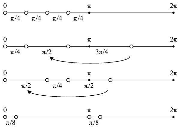
The optimal phase interval patterns for four relative phase offsets.

3.4. Error trend on the number of phase offsets

Essentially evenly distributed (π/M) phase offsets within the [0, π) interval were found to have the least estimation error when estimating the motion parameters A and θ. When the number of phase offsets M changes, the error follows the trend of one over the square root of M (Palmer, 1912, Pugh, 1966), while the conditioning stays the same. This trend indicates that the more data acquired, the more accurate the reconstructed phase and amplitude. The error decrease is significant when the number of phases is small. As the number increases, the error reduction with M slows and not much difference is found in the reconstructed results. Thus, it may not be necessary to use large numbers of phase offsets when acquiring raw MRE data. By estimating the noise level in the acquisition, the number of phase offsets required for a given accuracy can be determined.

4. Experimental results

Two phantom data sets, one with N = 16 and the other with N = 32, were obtained to test the simulation results. In vivo breast data obtained with N = 16 were also considered. Subsets of two and three relative phases were then extracted from these data sets and the motion reconstruction performance using fewer relative phase offsets were compared with that using all of the offsets. The shear modulus elastograms obtained with different numbers of phase offsets were also compared. All of the parameters affecting the elasticity reconstructions, including smoothing, regularization and spatial filtering (Doyley et al 2007) were kept the same for all cases.

4.1. Phantom data I: homogeneous case

A homogeneous gel was used to validate the simulation results. N = 16 evenly distributed relative phase offsets were acquired on a GE 1.5T MR scanner using a gradient echo pulse sequence (Weaver et al 2003) with phase cycling to remove the baseline phase. All possible combinations of 2 of the 16 phase offsets were reconstructed. The mean reconstruction difference ratios in amplitude between 2 and 16 phase offsets (with error bars) are shown in figure 5. The variation in per cent difference was caused by the different starting phase offsets chosen for a fixed phase interval. The noise level in the measurement is approximately 50% so the error bars in figure 5 are proportionally higher than those in figure 1 where the noise is only 5%. Small variations in the mean difference ratio were found when the phase interval was π/2 or 3π/2. With other intervals, large variations in the mean difference ratio can be seen in the figure. Thus the calculated motion is most stable when Δφ is π/2 or 3π/2.

Figure 5.

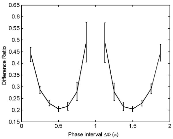
The mean values of estimation errors (with error bars) versus different phase intervals from a phantom experiment.

The motion map for one slice of gel is shown in figure 6 with estimation from 16 (left) and 2 (middle) phase offsets. In the middle image, the phase offsets are the first and the fifth, which have a phase interval of π/2, but the use of any of the phase offsets with the same intervals produces similar results. The right image is the difference between the two former images. The acquisition time is decreased by a factor of 8 when using two phase offsets whereas the motion estimation results have a difference of 8.3%.

Figure 6.

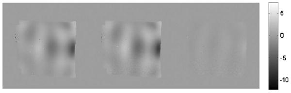
The displacement estimated from 16 (left) and 2 (middle) phase offsets; the right image is the subtraction of the former two images.

4.2. Phantom data II: cone inclusion

A block phantom with a cone inclusion was imaged on a Philips 3T MR scanner using a spin echo sequence (Sinkus et al 2000) and N = 32 evenly distributed relative phase offsets. The motion was reconstructed from all possible combinations of 3 of the 32 phase offsets. The mean reconstruction difference ratios in amplitude between 3 and 32 phase offsets are shown in figure 7. Similar noise patterns were found when the phantom results were compared with simulation results. The motion amplitude map for one slice of the phantom is shown in figure 8 with estimation from 32 (left) and 3 (middle) phase offsets. Both of them clearly show the big cone pattern and the difference image is shown on the right. In the middle image, the phase offsets are the 2nd, the 8th and the 16th, which have phase intervals of approximately π/3. Compared with the 32 phase offset image, the acquisition time from the 3 phase offset image is decreased by a factor of 10 whereas the motion estimation results have a 12.74% relative error. Although the error level is increased, the motion map retains the same features as the map from the full phase offset. The baseline phase variation was removed from the data in generating figures 7 and 8 to make it comparable to the other results where phase cycling was employed.

Figure 7.

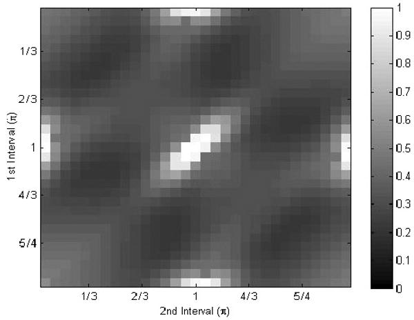
Noise pattern in the estimated amplitude for Tofu when three relative phases are used.

Figure 8.

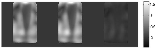
The motion amplitude estimated from 32 (left) and 3 (middle) phase offsets; the right image is the difference between the former two images.

4.3. In vivo results

Sixteen evenly distributed relative phase offsets were acquired on a GE 1.5T MR scanner from a volunteer. All possible combinations of 2 of the 16 phase offsets were reconstructed. The mean reconstruction difference ratios in displacement between 2 phase offsets and 16 phase offsets (with error bars) are shown in figure 9. Both the mean of difference ratios and the variations of difference ratios were found to be small, when the phase interval was around π/2 or 3π/2. For intervals that are near the ‘poles’, large variations in the mean difference ratio can be seen. In order to reduce the noise effect, a threshold was used to filter out the region that has a difference ratio larger than 5.

Figure 9.

The estimation errors versus different phase intervals from an in vivo exam when two phases are used.

The estimation results for three relative phases are shown in figure 10. Similar to the phantom results, the first and second intervals both contribute noise to the reconstruction. Similar noise patterns were found when in vivo results were compared with simulation results. Also, in order to reduce the noise effect, a threshold was used to filter out the region that has a motion displacement ratio larger than 5.

Figure 10.

Noise pattern in the estimated displacement when three relative phases are used.

The motion maps and shear modulus elastograms for one slice of acquisition are shown in figure 11, with estimation from 16 (left), 3 (middle) and 2 (right) phase offsets. In the right image, the phase offsets are the first and the fifth, which have a phase interval of π/2, but the use of any of the phase offsets with the same intervals produced similar results. In the middle image, the phase offsets are the first, the third and the seventh, which approximately have phase intervals of π/3. The motion map from 16 phase offsets is seen to be smoother than the ones with 3 and 2 phase offsets. However, the essential features of the image are the same when using 3 or 2 phase offsets. The shear modulus elastograms estimated from 16, 3 and 2 phase offsets are also seen to have similar features. The percentage difference in the shear modulus was calculated for each pixel and averaged over all pixels reconstructed in the slice. Reducing the number of phase offsets from 16 to 3 results in a 9.35% change in the shear modulus. Reducing the number of phase offsets from 16 to 2 results in a 10.05% change in the shear modulus. However, the acquisition time would be reduced by a factor of 5 when three phase offsets were used or by a factor of 8 when two phase offsets were used. It should be noted that, when the viscosity is being estimated, it might be more sensitive to noise than the elasticity.

Figure 11.

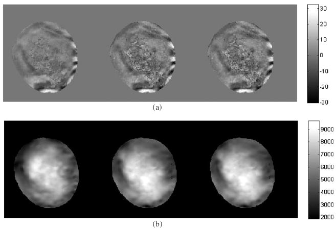
(a) The motion maps (in microns) estimated from 16 (left), 3 (middle) and 2 (right) phase offsets. (b) The shear modulus elastograms (in Pa) estimated from 16 (left), 3 (middle) and 2 (right) phase offsets.

5. Discussion

The reduced motion encoding (RME) method allows acquisitions with only two phases between the motion and the motion encoding gradients which significantly reduces the imaging time. However, the flexibility that RME provides is potentially much more significant. Many patterns of acquired phases could yield almost optimal SNR. In particular, the flexibility allows either a small number of high SNR measurements, such as spin echo measurements, or a larger number of lower SNR measurements, such as gradient echo measurements, to be employed.

The future work will focus on exploiting the flexibility found in the pattern of phases to adapt the method for specific clinical applications. RME offers flexibility that will be extremely useful when physiology imposes acquisition limitations. For example, MRE of the myocardium involves three cyclical processes: cardiac motion, the motion encoding gradients and the vibratory motion. MRE might allow retrospectively gated MRE acquisitions to be acquired in much less time because the fixed phase relationships between the vibratory motion and the motion encoding gradients would not be required. In addition, the method can also deal with interrupted acquisitions with incomplete clinical data. Another application would be to reduce sensitivity to phase wrapping for large vibratory motion. Further efforts are needed to investigate the relationship between phase pattern and the maximum unwrappable amplitude. The effects of baseline phases which would require phase cycling also require attention especially when comparing spin and gradient echo acquisitions.

6. Conclusion

Magnetic resonance elastography (MRE) measures mechanical vibrations by acquiring phase images at multiple relative phase offsets. The acquisition time of conventional MRE can be extraordinary long which could be an insuperable obstacle for MRE being applied routinely in the clinic. Thus reduction of acquisition time is an important goal for clinical MRE.

The RME method described here reduces imaging time significantly by reducing the number of phase offsets required. The minimum number of phase offsets required to estimate the motion is reduced from 4 to 2 if RME is employed. The noise decreases with the square root of the number of acquisitions as expected. Simulation and phantom results show that the estimation error is well characterized by the condition number of the transformation matrix. Generally for a given number of phase offsets φ acquired, the optimal samplings of φ to reduce noise are found to be essentially evenly distributed over the range [0, π) or over the range [0, 2π). Although sampling intervals near the ‘poles’ can cause large estimation error, a fairly wide distribution of sampling patterns was found to produce essentially optimal estimation errors, allowing a good deal of flexibility in selection of φ. In this sense, RME allows more flexible acquisitions than the conventional method and the acquisition time can be more closely matched to the required SNR.

References

- Beylkin G. On the fast Fourier-transform of functions with singularities. Appl Comput Harmon Anal. 1995;2:363–81. [Google Scholar]
- Doyley M, Feng Q, Weaver J, Paulsen K. Performance analysis of steady state harmonic elastography. Phys Med Biol. 2007;52:2657–74. doi: 10.1088/0031-9155/52/10/002. [DOI] [PubMed] [Google Scholar]
- Dubois E, Venetsanopoulos AN. New algorithm for radix-3 Fft. IEEE Trans Acoust Speech Signal Process. 1978;26:222–5. [Google Scholar]
- Dutt A, Rokhlin V. Fast Fourier-transforms for nonequispaced data. Siam J Sci Comp. 1993;14:1368–93. [Google Scholar]
- Hausmann R, Lewin SJ, Laub G. Phase-contrast Mr Angiography with reduced acquisition time—new concepts in sequence design. J Magn Reson Imaging. 1991;1:415–22. doi: 10.1002/jmri.1880010405. [DOI] [PubMed] [Google Scholar]
- Kruse SA, Smith JA, Lawrence AJ, Dresner MA, Manduca A, Greenleaf JF, Ehman RL. Tissue characterization using magnetic resonance elastography: preliminary results. Phys Med Biol. 2000;45:1579–90. doi: 10.1088/0031-9155/45/6/313. [DOI] [PubMed] [Google Scholar]
- Liu QH, Nguyen N. An accurate algorithm for nonuniform fast Fourier transforms (NUFFT's) IEEE Microw Guid Wave Lett. 1998;8:18–20. [Google Scholar]
- Manduca A, Dutt V, Borup DT, Muthupillai R, Ehman RL, Greenleaf JF. Reconstruction of elasticity and attenuation maps in shear wave imaging: an inverse approach. Medical Image Computing and Computer-Assisted Intervention—Miccai'98. 1998;1496:606–13. [Google Scholar]
- Manduca A, Muthupillai R, Rossman PJ, Greenleaf JF, Ehman RL. Image processing for magnetic resonance elastography. Proc SPIE. 1996;2710:616–23. [Google Scholar]
- Manduca A, Oliphant TE, Dresner MA, Mahowald JL, Kruse SA, Amromin E, Felmlee JP, Greenleaf JF, Ehman RL. Magnetic resonance elastography: non-invasive mapping of tissue elasticity. Med Image Anal. 2001;5:237–54. doi: 10.1016/s1361-8415(00)00039-6. [DOI] [PubMed] [Google Scholar]
- McCracken PJ, Manduca A, Felmlee J, Ehman RL. Mechanical transient-based magnetic resonance elastography. Magn Reson Med. 2005;53:628–39. doi: 10.1002/mrm.20388. [DOI] [PubMed] [Google Scholar]
- Muthupillai R, Lomas DJ, Rossman PJ, Greenleaf JF, Manduca A, Ehman RL. Magnetic-resonance elastography by direct visualization of propagating acoustic strain waves. Science. 1995;269:1854–7. doi: 10.1126/science.7569924. [DOI] [PubMed] [Google Scholar]
- Muthupillai R, Rossman PJ, Lomas DJ, Greenleaf JF, Riederer SJ, Ehman RL. Magnetic resonance imaging of transverse acoustic strain waves. Magn Reson Med. 1996;36:266–74. doi: 10.1002/mrm.1910360214. [DOI] [PubMed] [Google Scholar]
- Oppenheim AV, Schafer RW, Buck JR. Discrete-Time Signal Processing. Englewood Cliffs, NJ: Prentice-Hall; 1999. [Google Scholar]
- Palmer ADF. The Theory of Measurements. New York: McGraw-Hill; 1912. [Google Scholar]
- Prendergast RS, Levy BC, Hurst PJ. Reconstruction of band-limited periodic nonuniformly sampled signals through multirate filter banks. EEE Trans Circuits Syst I. 2004;51:1612–22. [Google Scholar]
- Pugh EM. The Analysis of Physical Measurements. Reading, MA: Addison-Wesley; 1966. [Google Scholar]
- Scoular SC, Fitzgerald WJ. Periodic nonuniform sampling of multiband signals. Signal Process. 1992;28:195–200. [Google Scholar]
- Sinkus R, Lorenzen J, Schrader D, Lorenzen M, Dargatz M, Holz D. High-resolution tensor MR elastography for breast tumour detection. Phys Med Biol. 2000;45:1649–64. doi: 10.1088/0031-9155/45/6/317. [DOI] [PubMed] [Google Scholar]
- Skare S, Hedehus M, Moseley ME, Li TQ. Condition number as a measure of noise performance of diffusion tensor data acquisition schemes with MRI. J Magn Reson. 2000;147:340–52. doi: 10.1006/jmre.2000.2209. [DOI] [PubMed] [Google Scholar]
- Steidl G. A note on fast Fourier transforms for nonequispaced grids. Adv Comput Math. 1998;9:337–52. [Google Scholar]
- Suga M, Matsuda T, Minato K, Oshiro O, Chihara K, Okamoto J, Takizawa O, Komori M, Takahashi T. Measurement of in vivo local shear modulus using MR elastography multiple-phase patchwork offsets. IEEE Trans Biomed Eng. 2003;50:908–15. doi: 10.1109/TBME.2003.813540. [DOI] [PubMed] [Google Scholar]
- Suzuki Y, Sone T, Kido KI. A new Fft algorithm of Radix-3, Radix-6, and Radix-12. IEEE Trans Acoust Speech Signal Process. 1986;34:380–3. [Google Scholar]
- Trefethen LN, Bau D., III . Numerical Linear Algebra. Philadelphia: SIAM; 1997. [Google Scholar]
- Van Houten EEW, Paulsen KD, Miga MI, Kennedy FE, Weaver JB. An overlapping subzone technique for MR-based elastic property reconstruction. Magn Reson Med. 1999;42:779–86. doi: 10.1002/(sici)1522-2594(199910)42:4<779::aid-mrm21>3.0.co;2-z. [DOI] [PubMed] [Google Scholar]
- Weaver J, Doyley M, Qin X, Van Houten E, Duncan L, Feng Q, Wang H, Kennedy F, Paulsen K. Improving MR elastography: measurement of cyclic motion using the frequency encoding gradients. Med Phys. 2003;30:1432–2. [Google Scholar]
- Weaver JB, Van Houten EEW, Miga MI, Kennedy FE, Paulsen KD. Magnetic resonance elastography using 3D gradient echo measurements of steady-state motion. Med Phys. 2001;28:1620–8. doi: 10.1118/1.1386776. [DOI] [PubMed] [Google Scholar]