Application of Reconstruction-Based Scatter Compensation to Thallium-201 SPECT:Implementations for Reduced Reconstructed Image Noise

Abstract

Scatter compensation in Tl-201 single photon emission computed tomography (SPECT) presents an interesting challenge because of the multiple emission energies and relatively large proportion of scattered photons. In this paper, we present a simulation study investigating reconstructed image noise levels arising from various implementations of iterative reconstruction-based scatter compensation (RBSC) in Tl-201 SPECT. A two-stage analysis was used to study single and multiple energy window implementations of reconstruction-based scatter compensation, and RBSC was compared to the upper limits on performance for other approaches to handling scatter. In the first stage, singular value decomposition of the system transfer matrix was used to analyze noise levels in a manner independent of the choice of reconstruction algorithm, providing results valid across a wide range of regularizations. In the second stage, the data were reconstructed using maximum-likelihood expectation-maximization, and the noise properties of the resultant images were analyzed. The best RBSC performance was obtained using multiple energy windows, one for each emission photopeak, and RBSC outperformed the upper limit on subtraction-based compensation methods. Implementing RBSC with the correct choice of energy window acquisition scheme is a promising method for performing scatter compensation for Tl-201 SPECT.

I. Introduction

The presence of scattered photons in single photon emission computed tomography (SPECT) projection data causes reduced contrast and a loss of quantitative accuracy in reconstructed images. A number of methods have been proposed to compensate for the effects of scatter [1]–[14], many of which involve estimating and subtracting the scattered component of the data. Such removal of scattered photons leads to an increase in statistical noise in the reconstructed image, causing degradation that may outweigh the benefits of performing the scatter correction [15]. An alternative to scatter subtraction is to model the scatter response function (SRF) during the reconstruction process [16]–[21]. This approach is called reconstruction-based scatter compensation (RBSC), and compensation is achieved, in effect, by mapping scattered photons back to their point of origin. Since all of the acquired counts are used, the noise increase found with scatter subtraction methods is avoided. In addition, RBSC can be used to reconstruct from energy windows which accept primarily scattered events. This allows for more counts to be included in the projection data, and there is potential to further reduce reconstructed image noise.

The accuracy of RBSC is dependent upon the accuracy of the scatter model used, and models have been developed that can provide very accurate three-dimensional (3-D) scatter compensation in SPECT [17], [18], [22]. The main disadvantage of RBSC is that the scatter models tend to be very computationally intensive, resulting in reconstruction times that are substantially longer than those required for other scatter compensation methods, and there exists a tradeoff between model accuracy and computational requirements. Recent advances in fast implementations of RBSC, such as using coarse-grid modeling approaches [23], unmatched projectors/backprojector pairs [23]–[25], and accelerated iterative algorithms [26], [27], have made RBSC reconstruction times clinically acceptable. Detailed evaluations of the accuracy of these methods are currently being performed by our group and others.

We have previously applied RBSC to Tc-99m SPECT [28], [29]. It was found that RBSC led to lower noise levels than subtraction-based scatter compensation methods. In addition, we found that nonphotopeak energy window data could be utilized to reduce image noise, but multiple energy windows were required to achieve this improvement. In this work we apply RBSC to the more complex situation of Tl-201 imaging, focusing upon the noise levels resulting from the various approaches studied. Other researchers have used subtraction-based approaches to scatter compensation when imaging Tl-201 [6]–[8], [30]–[34]. However, because of the relatively high proportion of scattered photons in Tl-201 projection data (on the order of 50% of the acquired counts), scatter subtraction results in an even higher noise increase than for Tc-99m imaging. Reconstruction-based scatter compensation has the potential to overcome this problem—by including and modeling the scattered events, they can be used in a productive manner.

The application of RBSC to Tl-201 imaging is more complicated than for Tc-99m. During thallium decay, photons are emitted across a wide range of energies, ranging from gamma rays at 135 and 167 keV to a series of X-rays at 69–83 keV. This complicates both attenuation and scatter compensation. The attenuation coefficient varies as a function of energy, and, due to beam hardening effects, the “average” attenuation coefficient for a given energy window will change as a function of source depth. The projection data for the lower energy windows will contain components donwnscattered from the gamma peaks in addition to components scattered from the nearby X-ray emissions. These effects, while complicating the situation, also mean that different energy windows will have very different primary and scattered components. In other words, the energies of the projection data carry additional information about the source distribution. This information can be preserved through the use of multiple energy windows, and may lead to both reduced bias and reduced noise levels as compared to using a single energy window.

In this work we investigate the utility of using RBSC, by modeling the scatter arising from each Tl-201 emission, to achieve scatter compensation in Tl-201 SPECT. We have studied implementing RBSC with a wide variety of single and multiple energy window data acquisition schemes, and compared the reconstructed image noise levels arising from each implementation. No model-specific evaluation of bias is included. The RBSC methods providing the lowest noise levels were compared with other approaches to handling scatter. Instead of singling out one of the many existing subtraction-based scatter compensation methods, we have compared RBSC to an idealized method which represents the upper limit on performance for the subtraction-based class of scatter compensation methods. In addition, we have compared RBSC to scatter discrimination and rejection methods which, although not achievable in practice, represent the upper limits on performance for these other approaches to handling scatter.

A two-stage analysis was used to evaluate the performance of each of the scatter compensation methods. In the first stage, singular value decomposition (SVD) of the system transfer matrix was used to study the noise levels resulting from each scatter compensation method. This SVD-based analysis has the benefit of being independent of the choice of reconstruction algorithm, and provides results that are summarized across a wide range of regularizations. Thus the SVD-based analysis provides flexible results that may hold for a wide range of imaging situations. In the second stage of the analysis, the data were reconstructed using the maximum-likelihood expectation-maximization (MLEM) algorithm, and the noise properties of the resultant images were studied. The results of the iterative analysis are shown to agree with the SVD-based analysis, and conclusions are drawn about the utility of using RBSC in Tl-201 SPECT.

II. Methods

A. Monte Carlo Simulations

The investigation was carried out using a Monte Carlo simulated phantom experiment. The phantom, shown in Fig. 1, was a 32 × 24-cm elliptical cylinder with infinite axial extent. It was filled with water and contained three cold rods (2-, 3-, and 5-cm diameter) in a uniform background of Tl-201 activity. This choice of phantom provided an extended scattering medium and a range of lesion sizes for contrast measurements, while remaining simple enough to expedite the analysis process. In particular, the axial uniformity of the phantom ensured that interslice scatter would be uniform along the axis. This allowed us to accurately include the 3-D effects of scatter while only simulating and reconstructing a single two-dimensional slice.

Fig. 1.

(a) The elliptical phantom activity image and (b) attenuation map. The phantom contained three cold rods, diameters 2, 3, and 5 cm, in a uniform background of Tl-201 activity, and the phantom was uniform in the axial direction.

The simulations were performed using the SIMIND Monte Carlo code [35]. The emissions arising from Tl-201 decay were simulated using the energies and relative abundances given in Table I. Up to four orders of scatter (both coherent and incoherent) were followed for the X-ray emissions, and up to ten orders were followed for the higher-energy gamma rays to accurately simulate downscatter to the lower-energy windows. The simulations were for a SPECT acquisition using a 40-cm-wide gamma camera equipped with a LEGP parallel hole collimator. The projection data were acquired into 64 bins, each 6.25-mm wide, and the scan was comprised of 128 views evenly spaced over 360°. The radius of rotation was 17 cm. The effects of attenuation, scatter and the detector response were included, but interactions within the collimator were not modeled (e.g., lead-fluorescence X-rays were not simulated). The camera used a 1.27-cm-thick NaI(Tl) crystal, and it was found that there was some loss of sensitivity for the higher energy photons due to incomplete absorption (9.1% loss at 167 keV, 1.3% loss at 135 keV, and negligible loss at the X-ray energies). The energy dependence of the detector sensitivity was accounted for in the reconstruction algorithm to preserve quantitative accuracy.

TABLE I.

Energies and Corresponding Relative Abundances for the Tl-201 Emissions that Were Used for the Monte Carlo Simulation and the Scatter Model Calculations

Energy (keV)	Relative Abundance (%)
68.89	25.5
70.82	43.3
80.11	15.0
82.58	4.1
135.3	2.5
167.38	9.6

The energy resolution of the camera was 11% full-width at half-maximum (FWHM) at 140 keV and varied as $1∕\sqrt{\text{energy}}$. A histogram of the energy spectrum of the simulated data is shown in Fig. 2, where the components arising from primary and scattered photons are indicated. The data were binned into the energy windows listed in Table II. In addition, the primary and scatter components of the projection data were stored separately to enable us to apply the idealized scatter 19compensation methods described in Section II-B2 below. A large number of photon histories (2.9 × 10¹⁰) were simulated to obtain essentially noise-free data. The data were later scaled and Poisson noise added to simulate a SPECT scan which acquired 3.0 × 10⁵ total counts in the “32% X-ray” window (this count level corresponds to 5.85 × 10⁵ total counts in the “Wide” energy window).

Fig. 2.

Histogram of the measured energy spectrum of the simulated projection data showing both the primary and scattered components at each energy.

TABLE II.

Description of the Energy Window Data Acquisition Schemes Studied for Each of the Scatter Compensation Methods

Name	No. Energy Windows	Energy windows used (keV)
RBSC Methods1:
32% X-ray	1	(64–88)
51% X-ray	1	(52–88)
4-X-ray	4	(64–70), (70–76), (76–82), (82–88)
6-X-ray	6	(52–58), (58–64), (64–70), (70–76), (76–82), (82–88)
X-ray+167	1	(64–88 + 150–185)
X-ray+G2	1	(64–88 + 120–185)
Dual-167	2	(64–88), (150–185)
Triple	3	(64–88), (120–150), (150–185)
Wide	1	(50–190)
TriScat	3	(64–88), (88–120), (120–185)
QuadScat	4	(64–88), (88–120), (120–150), (150–185)
5 Wins	5	(52–64), (64–88), (88–120), (120–150), (150–185)
Ideal Scatter Subtraction Methods2:
ISS Triple	3	(64–88), (120–150), (150–185)
Perfect Scatter Rejection Methods2:
PSR Triple	3	(64–88), (120–150), (150–185)
Perfect Scatter Discrimination Methods3:
PSD Triple	3 (6)	(64–88 primary), (120–150 primary), (150–185 primary), (52–88 scatter), (88–120 scatter), (120–185 scatter)

¹The SRF is modeled for these methods

²The SRF is not modeled for these methods

³The SRF is modeled for the scatter-only windows, but is not modeled for the primary-only windows

B. Reconstruction Methods

1) Reconstruction Algorithm

In the iterative analysis, the projection data were reconstructed using the MLEM algorithm with a rotation-based projector [17]. The effects of attenuation and detector response were modeled in the projector and backprojector for all cases, and scatter was also modeled when appropriate (refer to Section II-B2 for more information). To maintain quantitative accuracy, the energy dependencies of the attenuation coefficient and the detector efficiency were modeled in the projector and backprojector; in addition, the number of primary and scattered photons accepted by each energy window were also modeled. In practice, an approximate “average” attenuation coefficient would likely be used for each energy window to increase the speed of the projector and backprojector [36]. For the cases using more than one energy window, the data were reconstructed simultaneously to form a single image update at each iteration [37].

2) Scatter Compensation Methods

Reconstruction-based scatter compensation requires that the spatially-variant, object-dependent SRF be modeled during the reconstruction process. We have used the effective source scatter estimation (ESSE) model recently developed by Frey et al. [22]. The model works by calculating an “effective” scatter source, the attenuated projection of which gives the scattered component of the projection data. The model accounts for the spatial variance and depth dependence of the SRF, and has been found to work well for multiple- and large-angle scatters; the performance of the model for nonuniform attenuators is currently being evaluated. In order to apply the ESSE scatter model to Tl-201 imaging, the model was calibrated to account for each of the emission energies and relative abundances listed in Table I. For example, scatter in the “32% X-ray” window included components downscattered from the high-energy gamma emissions as well as components arising from the lower-energy X-ray emissions.

In order to gain an understanding of how the RBSC performance relates to that for other approaches to handling scatter, RBSC was compared to three idealized cases: i) perfect scatter rejection (PSR), ii) ideal scatter “subtraction” (ISS), and iii) perfect scatter discrimination (PSD). These three methods, described further below, are all idealized in that they cannot be achieved in practice. They represent the upper limit on performance for each approach to handling scatter. They are used to demonstrate how well modeling scatter (i.e., RBSC) performs compared to the best that could be achieved using other approaches to handling scatter.

The first of these methods, PSR, assumes that all scattered photons can be identified and rejected at acquisition, resulting in a data set comprised entirely of primary photon counts. This is the limiting case for scatter rejection methods, in which scatter discrimination (e.g., energy resolution) is used to limit the number of scattered photons that are accepted. In ISS, both primary and scattered photons are acquired, but it is assumed that the true mean (noise-free) scatter component is known. The scatter component is incorporated into the forward projection of the reconstruction algorithm to achieve scatter compensation [38], [39]; this is similar to performing prereconstruction scatter subtraction, but the compensation is performed during the reconstruction in order to maintain the Poisson structure of the noise in the projection data. The third method, PSD, is a hybrid of PSR and RBSC, in which it is assumed that photons can be tagged as either primary or scattered at acquisition. The primary counts are stored in one data set, and the scattered counts in another. The two data sets are then reconstructed simultaneously, using RBSC for the scattered data. This method is an alternative to PSR, and it is used to demonstrate the advantages of including scattered photons even if perfect scatter rejection capabilities existed.

We would like to reiterate that PSR, ISS, and PSD are idealized in that they require that either the true mean scatter component be known, or that primary and scattered counts can be perfectly differentiated at acquisition. In practice such ideals cannot be achieved, and the performance of practical implementations of these methods may fall well short of the idealized cases. For example, a practical implementation of scatter subtraction requires that the scattered component be estimated using the measured data. Hence the scatter estimate will be biased and contain a component due to the noise (the noise component may be relatively large or quite small depending upon the estimation method used); the result is a reconstructed image with both greater bias and somewhat higher variance than seen with ISS. In comparing RBSC to these idealized methods, we are holding RBSC to a very high standard.

C. Analysis Methods

Because SPECT images are inherently noisy, a regularization scheme is often applied to control the degree of noise in the image. This is usually achieved through the use of linear filters or by stopping iterative algorithms prior to convergence. There is a tradeoff between the degree of regularization applied (which suppresses some components of the image and leads to bias) and the degree of noise (variance) allowed to remain in the image. The choice of regularization is therefore task dependent. Since the degree of regularization affects the noise levels of the final image, it is important when comparing systems to evaluate their respective noise levels across the entire range of regularizations which may be desired. There is also an inherent difficulty in comparing iterative reconstructions which model different point responses: the images at each iteration may have very different bias and noise properties (i.e., are regularized differently). Since the rate of iterative recovery of image features may differ for each method, the images should not simply be compared at a given number of iterations.

In light of these considerations, we performed a two-stage analysis to evaluate the performance of RBSC relative to the other scatter compensation methods studied. The first stage of the analysis used SVD-based analysis methods to study reconstructed image noise levels in a manner that is independent of the choice of iterative reconstruction algorithm. In the second stage of the analysis, we studied the noise properties of images reconstructed using MLEM, taking care to account for the different rates at which image features are recovered with iteration. These analysis methods are described in more detail below.

1) SVD-Based Analysis Methods

In previous work with Tc-99m, we developed analysis methods based upon the SVD of the system transfer matrix [28], [29]. These methods are closely related to the generalized matrix inverse (GMI) reconstruction method [40], [41], and a brief summary of the methods is given here. The unfamiliar reader is encouraged to consult [28], [29], [40], and [41] for a more detailed description. The relevant statistically weighted imaging equation in SPECT can be written

$$\Psi \mathbf{F}\stackrel{‒}{\mathbf{x}}=\Psi \stackrel{‒}{\mathbf{p}}$$ (1)

where F is the system transfer matrix, Ψ is the statistical weighting matrix (the covariance matrix of the projections can be written as [Ψ^TΨ]⁻¹), $\stackrel{‒}{\mathbf{x}}$ is the vector of image pixels, and $\stackrel{‒}{\mathbf{p}}$ is the projection data vector. If the design matrix is decomposed using SVD: $\Psi \mathbf{F}\stackrel{\mathrm{SVD}}{\to }{\mathbf{USV}}^{\mathbf{T}}$, then the weighted least-squares reconstructed image ${\tilde{\mathbf{x}}}_{\mathbf{WLS}}$ can be obtained

$${\tilde{\mathbf{x}}}_{\mathbf{WLS}}={\mathbf{VS}}^{†}{\mathbf{U}}^{\mathbf{T}}\Psi \tilde{\mathbf{p}}$$ (2)

where $\tilde{\mathbf{p}}$ is the (noisy) measurement of the projection data. Here we have used the fact that U and V are unitary. The matrix S is diagonal, the diagonal elements of which are called the singular values and are arranged in descending order. The notation S^† denotes the pseudo-inverse of S, where the inverses of zero singular values have been set to zero, not infinity.

In addition to providing a means for reconstruction, the SVD provides a wealth of information about the imaging system. We have exploited this by calculating a metric called the “variance spectrum” $({\text{VARSPEC}}_i={\left[{\left({\mathbf{S}}_c{\mathbf{V}}_c^{\mathbf{T}}{\mathbf{VS}}^{†}\right)}_{ii}\right]}^2)$, which is calculated relative to a common singular vector basis (the common singular values and singular vectors are denoted by S_c and V_c, respectively). This metric summarizes the noise levels of GMI reconstructed image components across a wide range of regularizations. Each element of the VARSPEC metric is the variance of the GMI reconstructed image component in the direction of a common singular vector; the number of the singular vector and its corresponding singular value is referred to as the singular value index (i). The common basis allows for relative comparisons to be made; i.e., it converts the VARSPEC metric to a relative measured of reconstructed image variance. This approach provides fundamental results which are independent of the choice of reconstruction algorithm, and allows us to decouple bias properties from the noise analysis of the images.

An analogy can be drawn between the VARSPEC metric and the Fourier-based noise power spectrum [42]. Both of these metrics summarize the noise levels of a system, and both can be compared to corresponding signal power spectra to obtain information about the relative power of the signal and noise. Unlike the Fourier-based noise power spectrum, the VARSPEC metric does not assume stationarity of the noise, and it does not contain information about the noise correlation.

In this paper, the VARSPEC metric was calculated for each of the energy window schemes and scatter compensation methods listed in Table II. The transfer matrices were computed using the same projector as was used for the MLEM reconstructions, and statistical weighting was performed using the Monte Carlo simulated projection data as described in [28]. For the common basis, we chose to use the left singular vectors obtained from the SVD of the “32% X-ray” window transfer matrix. The SVD's and all other calculations were performed on a Cray T90 using Cray single precision (64-bit floating point). The VARSPEC metric is used in this paper to summarize the relative noise levels for each of the energy window schemes and scatter compensation methods studied.

2) Analysis of Iterative Reconstructions

The SVD-based analysis methods described above provide general and fundamental information about relative noise levels arising from the various scatter compensation methods studied. To lend weight to the results, a separate analysis of iteratively reconstructed images has been performed. Images were reconstructed using the MLEM algorithm and each of the scatter compensation methods and energy window schemes previously described. The contrast and noise properties of these images were then analyzed, taking care to account for the different rates of iterative recovery of image features for the methods.

In order to measure the image contrast, noise-free projection data were reconstructed out to 1000 iterations. Regions-of-interest (ROI's) were drawn within each cold rod and across the phantom background. The contrast ratio (CR) was then calculated for each rod as

$$\mathrm{CR}\equiv \mid \frac{\text{object}-\text{background}}{\text{object}+\text{background}}\mid$$ (3)

where “object” and “background” represent the mean pixel value in the corresponding ROI. The CR was calculated as a function of iteration, and provides a measure of the rate at which image contrast is recovered with iteration.

As a measure of the noise level of the reconstructed images, the variance of each pixel of the reconstructed image was estimated. This was done by reconstructing 100 independent noise realizations of the data and estimating the variance image at each iteration. As mentioned earlier, the rate of iterative recovery of image features depends upon the shape of the response function modeled in the projector and backprojector. Hence, it may not be valid to compare the reconstructed variance images at the same iteration, as images at a given iteration may be regularized differently. We have chosen to evaluate the variance of the reconstructions as a function of how image contrast is recovered with iteration. While this does not account for other components of bias, the results are more meaningful than simply comparing the images at the same iteration. Another possibility would have been to compare the images as a function of spatial resolution recovery; however, since scatter has a great effect upon image contrast, we feel the former comparison is more meaningful. Thus, the noise levels of the different methods will be compared by plotting the summed variance across the phantom background as a function of reconstructed image contrast at each iteration.

III. Results

A. SVD Analysis

As described in Section I, it may be advantageous to use multiple energy windows when imaging isotopes that have more than one emission peak. Since this is the case with Tl-201 imaging, we have studied implementing RBSC with a variety of single and multiple energy window data sets (Table II). These energy window schemes were chosen to demonstrate the effects of using the X-ray photopeaks alone, of including the higher-energy gama-ray photopeaks, and of including nonphotopeak (“scatter”) energy windows as well. In the following sections we use the VARSPEC metric to study the noise levels arising from each implementation of RBSC, and then compare the noise levels of the best RBSC methods to those for PSR, ISS, and PSD. Recall that the VARSPEC metric measures reconstructed image variance relative to the “32% X-ray” window RBSC method.

1) Comparison of X-Ray Photopeak Windows

We have calculated VARSPEC's for the RBSC methods that use projection data restricted to the X-ray photopeak region of the energy spectrum. The results are shown in Fig. 3. Two of the methods used a single energy window (“32% X-ray” and “51% X-ray”), and the remaining methods used multiple energy windows (“4 X-ray” and “6 X-ray”). The “32% X-ray” window resulted in a lower VARSPEC than for the “51% X-ray window.” This was because, even though the “51% X-ray” window had more counts, the additional counts were primarily due to scattered photons. The additional scattered counts had the effect of degrading the system response function, and this degradation outweighed the benefit of including more counts. Similar effects have been observed for Tc-99m imaging [28].

Fig. 3.

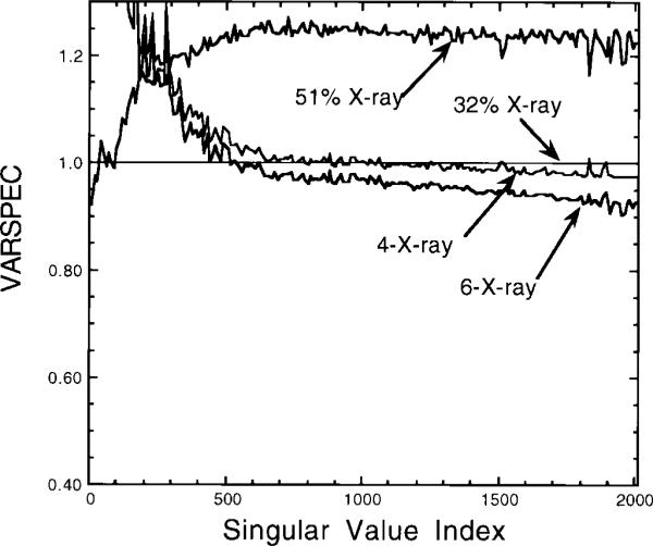
Comparison of VARSPEC's for four RBSC methods which use only photons near the X-ray emission region of the energy spectrum. Refer to Table II for descriptions of the methods.

A different trend was seen for the multiple-window methods. The “4 X-ray” and “6 X-ray” energy window data sets spanned the same energy ranges as the “32% X-ray” and “51% X-ray” windows, but did so using four and six energy windows, respectively. In this case, it was found that the wider energy range (“6 X-ray”) resulted in a lower VARSPEC than did the narrow energy range (“4 X-ray”). By using multiple energy windows, the additional scattered photons were not lumped in with the primaries, so the degradation mentioned above did not occur. The “6 X-ray” window method was found to give the lowest VARSPEC for the methods studied which use only the X-ray photopeak region of the energy spectrum.

2) Inclusion of Gamma Ray Photopeak Windows

Fig. 4 shows VARSPEC's for the RBSC methods which include one or both of the higher-energy gamma-ray photopeaks in addition to the X-ray photopeaks. For the single-window methods (“X-ray + 167” and “X-ray + G2”) the higher energy data were summed with the X-ray window data to yield a single, discontinuous energy window. The other cases (“Dual-167” and “Triple”) used multiple energy windows. In all cases, including the gamma-ray photopeaks led to lower VARSPEC's than using only the X-ray photopeaks. The best performance was obtained when using three energy windows, one for each emission energy (“Triple”). This result supports our hypothesis that the energy of the data carries some useful information. When using separate energy windows for the different regions of the energy spectrum, some of this information is preserved. The result is a system that is less sensitive to noise, leading to reconstructed images with lower variance.

Fig. 4.

VARSPEC plots for the methods which included gamma-ray photopeak energies in addition to X-ray energies. The 32% X-ray window VARSPEC is also shown for comparison.

3) Inclusion of Nonphotopeak Window Scatter Data

When using RBSC with accurate scatter models, energy windows containing primarily scattered photons can be included in the reconstruction without adversely affecting image quality [28], [29]. Fig. 5 shows VARSPEC's for the methods which include nonphotopeak regions of the energy spectrum in addition to the photopeak regions. Several single and multiple energy window cases are shown. Using a single wide energy window (“Wide”) resulted in the highest variance, worse than using only an X-ray window. Again, this is consistent with the result that lumping additional scattered photons in with primaries is not a good approach. However, using separate energy windows for nonphotopeak (scatter) and photopeak regions of the energy spectrum resulted in much lower variances. The case with five energy windows (“5 Wins”) performed the best, resulting in a VARSPEC that was somewhat lower than that achieved when not including scatter windows. This result agrees with trends observed with Tc-99m—if separate energy windows are used for photopeak and nonphotopeak regions of the energy spectrum, then nonphotopeak scattered counts can be used productively. However, if the scatter counts are lumped in with the primaries, the resultant degradation of the system response function makes the system more sensitive to noise, and this effect outweighs the benefits of including more counts.

Fig. 5.

Plots of the VARSPEC's for the methods which include scatter windows in addition to photopeak energy windows. The 32% X-ray window is included for comparison.

4) Comparison of RBSC to Other Approaches of Handling Scatter

Having studied a number of implementations of RBSC for thallium imaging, we turn now to comparing the best RBSC method with other, idealized approaches to handling scatter (ISS, PSR, and PSD). The cases using multiple energy windows (three photopeak windows, plus nonphotopeak windows for RBSC and PSD) provided the most interesting results, and the VARSPEC's for these methods are shown in Fig. 6. Similar trends between scatter compensation methods were observed when acquiring into a single energy window (results not shown). The VARSPEC for ISS was the highest, due to the noise increase resulting from the subtraction step. Separation of scatter (PSD) resulted in a slightly lower variance than did scatter rejection (PSR). This is evidence that the outright rejection of scatter may not be the best method. These results are academically interesting, and may help guide future research in scatter compensation. Of practical interest, RBSC performed better than ISS, but fell well short of both PSR and PSD. This is an indication that improving the scatter discriminating capabilities of SPECT cameras (e.g., by improving energy resolution) could lead to a reduction in reconstructed image noise levels [43].

Fig. 6.

Comparison of the VARSPEC's for the various scatter compensation methods using multiple energy windows. Each method used three photopeak windows, and RBSC and PSD include additional scatter windows as well.

B. Iterative Reconstructions

The results of the SVD-based analysis were corroborated by analyzing the contrast and variance of iterative MLEM reconstructions. We present here the results for the multiple window implementations of RBSC, ISS, PSR, and PSD. The contrast ratios for the 5-cm cold rod are plotted as a function of iteration in Fig. 7. Though all of the scatter compensation methods recovered very good contrast, the rate of iterative recovery of image contrast differed for each of the methods. For example, contrast recovery was slowest for RBSC. Because scatter is modeled for RBSC, the modeled point response function was wider, and iterative recovery of image features was slowed.

Fig. 7.

Contrast ratio of the 5-cm cold rod plotted as a function of iteration number for each of the various scatter compensation methods. The energy window schemes were the same as in Fig. 6.

In Fig. 8 we show reconstructed images for each of the scatter compensation methods. Fig. 8 includes reconstructions from both noise-free and noisy data, and reconstructed variance images over 100 noise realizations are also included. Each image is shown at the iteration which provided a contrast ratio of 0.6 in the 5-cm rod (80 iterations for RBSC, 50 for ISS, 30 for PSR, and 100 for PSD). At these respective iterations, the noise-free reconstructions were found to be qualitatively very similar. However, the noisy and variance images exhibit some interesting effects: there were substantial differences in the structure and magnitude of the variance images, and the noisy images had some differences in noise texture. We have not performed a detailed study of the differences in noise correlation arising from the different treatments of scatter, and it should be noted that such differences would be expected to affect the usefulness of reconstructed images for tasks such as lesion detection.

Fig. 8.

Sample MLEM reconstructed images for each scatter compensation method at the iteration which had CR = 0.6 (refer to Fig. 7). Columns, left to right: RBSC 5 Wins, ISS Triple, PSR Triple, and PSD Triple. Rows, top to bottom: noise-free data, noisy data, and variance images. All of the images have been displayed using the same grayscale, shown at the right.

To quantify the differences in the variance images, the pixels in the background were summed and plotted as a function of contrast ratio of the 5-cm rod. Plotting versus contrast ratio as opposed to versus iteration accounts for some of the effects of differing iterative convergence rates, and helps ensure a meaningful comparison can be drawn. The results are shown in Fig. 9. The observed trends agree with the variance spectra results; namely, ISS resulted in the highest reconstructed image variance, followed by RBSC, PSR, and PSD. In addition to differences in the overall variance, the structure of the variance images differed for each method. The methods which include scatter modeling (RBSC and PSD) generally had lower variance near the image center than at the image edges, whereas the variance was more radially constant for the cases which did not model scatter (PSR and ISS). Such an effect may have important consequences when the organ being imaged is near the center of the body, e.g., cardiac imaging. Further research is required to determine if RBSC methods provide greater benefit for imaging objects deep within the body.

Fig. 9.

Summed variance in the phantom background plotted as a function of contrast ratio recovery for each of the scatter compensation methods. The methods and energy window schemes are the same as used in Figs. 6–8.

IV. Discussion

The results of the preceding sections have allowed us to draw conclusions about the utility of performing RBSC in Tl-201 SPECT, as compared to using other approaches to handling scatter. The agreement between the SVD-based analysis methods and the analysis of the iterative reconstructions suggests that similar results may be found for a wider range of imaging situations and reconstruction algorithms; however, the results of this paper were based solely upon a single simulated source distribution with uniform scattering media. While the results may be similar for other source and attenuation distributions, further evaluation is required before the conclusions of this work can be generalized. The specific conclusions drawn in this paper are intended to guide development of future approaches to performing scatter compensation in Tl-201 SPECT, and a number of remaining issues need to be addressed before any practical applications of RBSC should be considered.

The study was limited to a simulation experiment of a phantom for which the scatter models worked very well. Modeling scatter for nonuniform attenuators is more difficult, and bias may become a more significant issue in these situations. In addition, for Tl-201 imaging, modeling scatter arising from the multiple emission peaks is more difficult than if there were only one emission energy. Though the ESSE scatter model worked very well in this regard, other scatter models may not generalize so easily. A number of researchers are currently developing and evaluating scatter models for use in SPECT, and the tradeoff between bias and computational effort needs to be fully evaluated for each model. In addition, further evaluation of fast implementations of RBSC needs to be performed.

We have shown that using multiple energy windows can result in lower reconstructed image noise levels in many situations, but we have not addressed the issue of increased reconstruction times that result from the use of multiple energy windows. The time required for reconstruction will scale roughly with the number of energy windows, which may prohibit the use of a large number of energy windows in a clinical setting. For example, the moderate reduction of noise levels obtained by including additional nonphotopeak energy windows is unlikely to warrant the corresponding increase in reconstruction times. Additionally, many clinical systems offer a limited number of energy windows (2–4), and disk storage space may place an additional limit on the number of windows that may be practical. In light of these considerations, performing Tl-201 SPECT with RBSC and two or three energy windows (e.g., “Dual-167” or “Triple” from Table II) may be a good approach.

V. Summary and Conclusions

We have investigated applying reconstruction-based scatter compensation to Tl-201 SPECT using a variety of energy window schemes, and compared the resultant reconstructed image noise levels to those arising from other, idealized approaches to handling scatter. This was done using a simulated phantom experiment with uniform scattering media. A fundamental analysis was first performed using SVD-based analysis methods, and the results were corroborated through analysis of the contrast and variance of iterative MLEM reconstructions. Due to the multiple emission energies of Tl-201, using RBSC with multiple energy windows was found to result in images with lower variance than was found when using a single energy window. In particular, using separate windows for the X-ray photopeaks and the gamma photopeaks was advantageous, and using additional nonphotopeak windows was moderately beneficial.

When compared with other approaches to handling scatter, RBSC was found to result in lower noise levels than could be obtained with scatter subtraction methods. However, other idealized methods (PSR and PSD) were found to outperform RBSC, indicating that improvements in imaging hardware (e.g., better energy resolution) could lead to improvements in image quality. In future work, the bias of RBSC scatter models need to be evaluated for nonuniform attenuators, and recently developed fast implementations of RBSC need to be validated. When this is accomplished, RBSC may potentially emerge as the scatter compensation method of choice in SPECT.

References

- [1].Jaszczak RJ, Greer KL, Floyd CE, Jr., Harris CC, Coleman RE. Improved SPECT quantitation using compensation for scattered photons. J. Nucl. Med. 1984;25:893–900. [PubMed] [Google Scholar]
- [2].Axelsson B, Msaki P, Israelsson A. Subtraction of Compton-scattered photons in single-photon emission computerized tomography. J. Nucl. Med. 1984;25:290–294. [PubMed] [Google Scholar]
- [3].Ichihara T, Ogawa K, Motomura N, Kubo A, Hashimoto S. Compton scatter compensation using the triple-energy window method for single-and dual-isotope SPECT. J. Nucl. Med. 1993;34:2216–2221. [PubMed] [Google Scholar]
- [4].King MA, Hademenos GJ, Glick SJ. A dual-photopeak window method for scatter correction. J. Nucl. Med. 1992;33:605–612. [PubMed] [Google Scholar]
- [5].Floyd CE, Jaszczak RJ, Greer KL, Coleman RE. Deconvolution of Compton scatter in SPECT. J. Nucl. Med. 1985;26:403–408. [PubMed] [Google Scholar]
- [6].Hutton BF, Osiecki A, Meikle SR. Transmission-based scatter correction of 180° myocardial single-photon emission tomographic studies. Eur. J. Nucl. Med. 1996;23:1300–1308. doi: 10.1007/BF01367584. [DOI] [PubMed] [Google Scholar]
- [7].Meikle SR, Hutton BF, Bailey DL. A transmission-dependent method for scatter correction in SPECT. J. Nucl. Med. 1994;35:360–367. [PubMed] [Google Scholar]
- [8].Narita Y, Iida H, Eberl S, Nakamura T. Monte Carlo evaluation of accuracy and noise properties of two scatter correction methods. Proc. 1996 IEEE Nuclear Science Symp. and Medical Imaging Conf.; Anaheim, CA. 1996. pp. 1434–1438. [DOI] [PubMed] [Google Scholar]
- [9].Msaki P, Axelsson B, Dahl CM, Larsson SA. Generalized scatter correction method in SPECT using point scatter distribution functions. J. Nucl. Med. 1987;28:1861–1869. [PubMed] [Google Scholar]
- [10].Ogawa K, Harata Y, Ichihara T, Kubo A, Hashimoto S. A Practical method for position-dependent Compton scatter correction in SPECT. IEEE Trans. Med. Imag. 1991;10:408–412. doi: 10.1109/42.97591. [DOI] [PubMed] [Google Scholar]
- [11].Koral KF. SPECT Compton-scattering correction by analysis of energy spectra. J. Nucl. Med. 1988;29:195–202. [PubMed] [Google Scholar]
- [12].Gagnon D, Todd-Pokropek A, Arsenault A, Dupras G. Introduction to holospectral imaging in nuclear medicine for scatter subtraction. IEEE Trans. Med. Imag. 1989;8:245–250. doi: 10.1109/42.34713. [DOI] [PubMed] [Google Scholar]
- [13].Hamill JJ, Devito RP. Scatter reduction with energy-weighted acquisition. IEEE Trans. Nucl. Sci. 1989;36 [Google Scholar]
- [14].Pretorius PH, Rensburg A. J. v., Aswegen A. v., Lotter MG, Serfontein DE, Herbst CP. The channel ratio method of scatter correction for radionuclide image quantitation. J. Nucl. Med. 1993;34:330–335. [PubMed] [Google Scholar]
- [15].deVries DJ, King MA, Soares EJ, Tsui BMW, Metz CE. Evaluation of the effect of scatter correction on lesion detection in hepatic SPECT imaging. IEEE Trans. Nucl. Sci. 1997;44:1733–1740. [Google Scholar]
- [16].Frey EC, Tsui BMW. A practical method for incorporating scatter in a projector–backprojector for accurate scatter compensation in SPECT. IEEE Trans. Nucl. Sci. 1993;40:1107–1116. [Google Scholar]
- [17].Frey EC, Ju ZW, Tsui BMW. A fast projector–backprojector pair modeling the asymmetric, spatially varying scatter response function for scatter compensation in SPECT imaging. IEEE Trans. Nucl. Sci. 1993;40:1192–1197. [Google Scholar]
- [18].Beekman F, Eijkman E, Viergever M, Borm G, Slijpen E. Object shape dependent PSF model for SPECT imaging. IEEE Trans. Nucl. Sci. 1993;40:31–39. [Google Scholar]
- [19].Beekman FJ, Kamphuis C, Viergever MA. Improved SPECT quantitation using fully three-dimensional iterative spatially variant scatter response compensation. IEEE Trans. Med. Imag. 1996;15:491–499. doi: 10.1109/42.511752. [DOI] [PubMed] [Google Scholar]
- [20].Floyd CE, Jaszczak RJ, Coleman RE. Inverse Monte Carlo: A unified reconstruction algorithm. IEEE Trans. Nucl. Sci. 1985;NS-32:779–785. [PubMed] [Google Scholar]
- [21].Welch A, Gullberg GT, Christian PE, Datz FL. A transmission map-based scatter correction technique for SPECT in inhomogenous media. Med. Phys. 1995;22:1627–1635. doi: 10.1118/1.597422. [DOI] [PubMed] [Google Scholar]
- [22].Frey EC, Tsui BMW. A new method for modeling the spatially-variant, object-dependent scatter response function in SPECT. Proc. 1996 IEEE Nuclear Science Symp. and Medical Imaging Conf.; Anaheim, CA. 1996. pp. 1082–1086. [Google Scholar]
- [23].Kadrmas DJ, Frey EC, Tsui BMW. Fast implementations of iterative reconstruction-based scatter compensation for fully 3-D SPECT reconstruction. Phys. Med. Biol. 1998;43(4):857–873. doi: 10.1088/0031-9155/43/4/014. vol. 43. 1998. [DOI] [PMC free article] [PubMed] [Google Scholar]
- [24].Kamphuis C, Beekman FJ, Viergever MA, van Rijk PP. Accelerated fully 3-D SPECT reconstruction using dual matrix ordered subsets (abstract) J. Nucl. Med. 1996;37:62P. doi: 10.1007/s002590050188. [DOI] [PubMed] [Google Scholar]
- [25].Zeng GL, Weng Y, Gullberg GT. Iterative reconstruction with attenuation compensation from cone-beam projections acquired via nonplanar orbits. IEEE Trans. Nucl. Sci. 1997;44:98–106. [Google Scholar]
- [26].Hudson HM, Larkin RS. Accelerated image reconstruction using ordered subsets of projection data. IEEE Trans. Med. Imag. 1994;13:601–609. doi: 10.1109/42.363108. [DOI] [PubMed] [Google Scholar]
- [27].Byrne CL. Block-iterative methods for image reconstruction from projections. IEEE Trans. Image Processing. 1996;5:792–794. doi: 10.1109/83.499919. [DOI] [PubMed] [Google Scholar]
- [28].Kadrmas DJ, Frey EC, Tsui BMW. Analysis of the reconstructibility and noise properties of scattered photons in Tc-99m SPECT. Phys. Med. Biol. 1997;42:2493–2516. doi: 10.1088/0031-9155/42/12/014. [DOI] [PMC free article] [PubMed] [Google Scholar]
- [29].Kadrmas DJ, Frey EC, Tsui BMW. An SVD investigation of modeling scatter in multiple energy windows for improved SPECT images. IEEE Trans. Nucl. Sci. 1996;43:2275–2284. doi: 10.1109/23.531892. [DOI] [PMC free article] [PubMed] [Google Scholar]
- [30].deVries DJ, King MA, Weinstein H. Scatter correction for Tl-201 cardiac imaging: A Monte Carlo investigation. J. Nucl. Med. 1994;35:192. [Google Scholar]
- [31].Floyd JL, Mann RB, Shaw A. Changes in quantitative SPECT Thallium-201 results associated with the use of energy-weighted acquisition. J. Nucl. Med. 1991;32:805–807. [PubMed] [Google Scholar]
- [32].Galt JR, Cullom SJ, Garcia EV. SPECT quantification: A simplified method of attenuation and scatter correction for cardiac imaging. J. Nucl. Med. 1992;33:2232–2237. [PubMed] [Google Scholar]
- [33].Hademenos GJ, King MA, Ljungberg M, Zubal GI, Harrell CR. A scatter correction method for Tl-201 images: A Monte Carlo investigation. IEEE Trans. Nucl. Sci. 1993;40:1179–1186. [Google Scholar]
- [34].Li J, Tsui BMW, Frey EC, Gullberg GT. Deconvolution scatter compensation for Thallium-201 fan-beam cardiac SPECT. Proc. 1995 IEEE Nuclear Science Symp. and Medical Imaging Conf.; San Francisco, CA. 1995. pp. 1175–1179. [Google Scholar]
- [35].Ljungberg M, Strand S-E. A Monte Carlo program for the simulation of scintillation camera characteristics. Comput. Meth. Prog. Biomed. 1989;29:257–272. doi: 10.1016/0169-2607(89)90111-9. [DOI] [PubMed] [Google Scholar]
- [36].Pretorius PH, King MA, Pan T-S, Hutton BF. Attenuation correction strategies for multi-energy photon emitters using SPECT. presented at IEEE 1996 Nuclear Science Symp. and Medical Imaging Conf.; Anaheim, CA. 1996. [Google Scholar]
- [37].Frey EC, Tsui BMW. Use of the information content of scattered photons in SPECT by simultaneous reconstruction from multiple energy windows. J. Nucl. Med. 1994;35:17. [Google Scholar]
- [38].Lange K, Carson R. E.M. reconstruction algorithms for emission and transmission tomography. J. Comput. Assit. Tomogr. 1984;8:306–316. [PubMed] [Google Scholar]
- [39].Bowsher JE, Johnson VA, Turkington TG, Jaszczak RJ, Floyd CE, Coleman RE. Bayesian reconstruction and use of anatomical a priori information for emission tomography. IEEE Trans. Med. Imag. 1996;15:673–686. doi: 10.1109/42.538945. [DOI] [PubMed] [Google Scholar]
- [40].Huesman RH, Gullberg GT, Greenberg WL, Budinger TF. Donner algorithms for reconstruction tomography. Lawrence Berkeley Lab. PUB-214; 1977. [Google Scholar]
- [41].Smith MF, Floyd CE, Jaszczak RJ, Coleman RE. Reconstruction of SPECT images using generalized matrix inverses. IEEE Trans. Med. Imag. 1992;11:165–175. doi: 10.1109/42.141640. [DOI] [PubMed] [Google Scholar]
- [42].Riederer SJ, Pelc NJ, Chelser DA. The noise power spectrum in computed tomography. Phys. Med. Biol. 1978;23:446–454. doi: 10.1088/0031-9155/23/3/008. [DOI] [PubMed] [Google Scholar]
- [43].Kadrmas DJ, Frey EC, Tsui BMW. Effects of improving energy resolution upon the performance of scatter compensation techniques in SPECT (abstract) J. Nucl. Med. 1997;38(5):89P. [Google Scholar]