Analysis of the Reconstructibility and Noise Properties of Scattered Photons in Tc-99m SPECT

Abstract

Since scattered photons carry degraded spatial information, scatter is typically considered a source of contamination in SPECT. However, with the advent of scatter modeling methods and reconstruction-based scatter compensation (RBSC), it may be possible to utilize scattered data in a productive manner. In this work we analyze the reconstructibility of scattered photon projection data and investigate the potential for using scattered photons to reduce the noise levels of SPECT images. We have simulated projection data for an elliptical phantom containing three cold rods in a uniform background of Tc-99m activity. A variety of photopeak and scatter energy windows were formed, as well as corresponding RBSC transfer matrices. Each statistically weighted matrix was decomposed using SVD and analyzed in terms of reconstructibility and noise properties. Results indicate that scattered photons contain sufficient information to reconstruct the source activity, but the scatter-only matrices are very poorly conditioned. We have also evaluated several methods of utilizing scattered events via RBSC, and compared them with other, idealized methods of handling scatter. It was found that scattered photons can be used productively when photopeak and non-photopeak data are separated through the use of multiple energy windows. The RBSC methods outperformed ideal scatter subtraction, but fell short of methods which assume perfect discrimination between scattered and primary events. The knowledge gained by this study may help guide future research and lead to better approaches to handling scatter in SPECT.

1. Introduction

One of the most difficult image degrading factors to account for in SPECT imaging is that some photons will scatter in the patient and then be detected. These scattered photons carry degraded spatial information, so energy discrimination is often used to reduce the number that are detected. However, imperfect energy resolution coupled with the presence of small angle and coherent scatter limits the extent to which scattered photons can be rejected. In some situations, e.g. Tl-201 imaging, scattered events can exceed 50% of the acquired counts. If adequate compensation is not performed, scatter leads to a loss of contrast and inaccurate quantitation in reconstructed images.

A number of methods have been proposed to compensate for scatter (Axelsson et al 1984, Jaszczak et al 1984, Floyd et al 1985b, Msaki et al 1987, Koral et al 1988, Gagnon et al 1989, Hamill and Devito 1989, Ogawa et al 1991, King et al 1992, Pretorious et al 1993). Most of these methods attempt to estimate the scatter contamination and then remove it using either subtraction or deconvolution techniques. There have been a number of studies comparing these methods (Yanch et al 1988, Gilardi et al 1988, Ljungberg et al 1990, Frey et al 1992, Frey et al 1993b, Ljungberg et al 1994). The primary concerns affecting these methods are: (i) the scatter estimates may be inaccurate, leading to bias in the reconstructed image; and (ii) the scatter compensation is often accompanied by a substantial increase in statistical noise. In addition, many of the methods require estimating parameters that may change for each patient and imaging protocol.

With the advent of faster computers and accelerated iterative reconstruction algorithms, a different approach to scatter compensation is receiving much attention. Reconstruction-based scatter compensation (RBSC) is a technique in which the scatter response function (SRF) is modeled during the reconstruction process (Floyd et al 1985a, Bowsher and Floyd 1991, Smith et al 1992b, Beekman et al 1993, Frey and Tsui 1993, Frey et al 1993a, Welch et al 1995). In effect, scatter compensation is performed by mapping scattered photons back to their point of origin. Compared to subtraction-based scatter compensation methods, RBSC has been shown to produce images with both less bias and reduced variance (Frey et al 1992). The main disadvantage of RBSC is the relatively large computational cost of computing the scatter contribution at each iteration, which becomes prohibitive when performing fully 3D reconstructions. Several researchers are currently investigating methods of modeling the SRF which are fast and accurate for non-uniform attenuators.

Several investigators have studied the spatial distribution of Compton scattered photons using Monte Carlo methods (Floyd et al 1984, Frey and Tsui 1991). It was found that the SRF contains a peaked component, even for energies well below the photopeak. This suggests that photons which are scattered retain some spatial information about the source activity distribution. The premise of this work is that this information can be used, by including scattered photons and modeling the SRF during the reconstruction, to improve the noise characteristics of SPECT imaging. There has been some evidence presented by other researchers supporting this hypothesis. Smith et al (1992b) investigated using two windows, a photopeak window and a lower energy scatter window, to simultaneously constrain Tc-99m activity estimates. Their experiment essentially performed RBSC using two energy windows and the generalized matrix-inverse (GMI) reconstruction method. The paper focused on the bias of the reconstructed image, and they found a slight improvement compared to using dual energy window scatter subtraction. Though statistical noise was not directly addressed in the text, RBSC resulted in smaller uncertainties in their activity estimates than did scatter subtraction.

When using iterative reconstructions, the rate at which image features are recovered depends upon the response function modeled in the projector and backprojector. Since images at the same iteration may have very different bias and noise properties (i.e., they are regularized differently), it is difficult to compare their noise levels in a meaningful way. In previous work (Kadrmas et al 1996) we developed methods, based upon the singular value decomposition (SVD) of the system transfer matrix, to investigate the reconstructibility and noise properties of SPECT systems employing a variety of single and multiple energy window schemes. The SVD-based analysis methods provide a means for meaningful comparison of noise levels that is valid across a wide range of regularizations. The results indicated that RBSC led to lower image noise than scatter subtraction. Perfect scatter rejection (the ideal and physically unachievable case in which only unscattered photons are acquired) had the lowest noise level of the methods studied, even though this case had the lowest number of counts. It was also demonstrated that low energy scattered photons had some potential for being used to reduce image noise. However, in order to fully investigate the potential for scattered counts to reduce SPECT noise levels, it was found necessary to model the statistics more accurately by including statistical weights in the imaging equation.

In this work we employ a systematic approach to investigate the potential benefits of including scattered photons in SPECT. In doing so, we have extended the SVD-based analysis methods to include statistical weights in the imaging equation. The investigation can be broken down into four stages: (i) analysis of the reconstructibility and noise properties of scattered photon data near the photopeak; (ii) evaluation and comparison of several methods of handling the scattered photons investigated in (i); (iii) analysis of the reconstructibility and noise properties of scattered photons in energy windows below the photopeak; and (iv) evaluation and comparison of methods which use low energy photons in addition to photopeak data. We have made an attempt to find energy window schemes which lead to the lowest noise levels when using RBSC, and we compare the best RBSC methods with other, idealized methods of handling scatter. We also investigate a new method, RBSC with scatter discrimination, which is shown to outperform scatter rejection methods. This method is not achievable in practice, but it illustrates the limiting potential for using scattered photons in conjunction with primary photons. Finally, we discuss some of the limitations of our investigation and draw conclusions based upon this work..

2. Theory

This paper relies heavily upon SVD-based analysis methods which are valid for a wide range of regularizations and are independent of the choice of iterative reconstruction algorithm. In this section we extend the theoretical formulation of Kadrmas et al (1996) to include statistical weighting in the imaging equation, and derive expressions for the (weighted) signal power and variance metrics. A basic introduction to weighted generalized matrix-inverse (W-GMI) reconstruction methods using SVD is also presented, but the unfamiliar reader is encouraged to consult one or more of the references (Huesman et al 1977, Golub and Loan 1989, Press et al 1988, Smith et al 1992) for more information on the subject.

2.1. Weight Least Squares Estimation Using SVD

The weighted projection image formation process in SPECT may be written in matrix-vector form as (Gullberg et al 1995):

$$\Psi \mathbf{F}\stackrel{\rightharpoonup }{\mathbf{y}}=\Psi \stackrel{\rightharpoonup }{\mathbf{p}},$$ (1)

where,

F ≡ the M × N photon transfer matrix,

$\stackrel{\rightharpoonup }{\mathbf{y}}$ ≡ the N × 1 true image vector,

$\stackrel{\rightharpoonup }{\mathbf{p}}$ ≡ the M × 1 mean projection data vector, and

Ψ ≡ the M × M weighting matrix.

The product ΨF is known as the design matrix. The weighting matrix, Ψ , is diagonal, and the diagonal elements are the statistical weights. The Poisson statistics of the projection data can be approximated using Gaussian statistics by choosing the variance of each projection datum to be its mean (noise-free) value. The corresponding weights are then given by inverting the resultant standard deviations. In the case of typical SPECT, for which the noise in the projection data is uncorrelated, Ψ has an interesting property—the product Ψ^TΨ is equal to Φ⁻¹ , where Φ is the covariance matrix of the projection data. This notation for Ψ^TΨ will be used below. To avoid division by zero problems, data with mean value less than or equal to 0.1 were assigned a weight of $1.0∕\sqrt{0.1}$ in this paper. This threshold also avoids potential numerical errors for data which are very near to zero.

The WLS solution is readily obtained from eq. (1) by decomposing the design matrix using SVD:

$$\Psi \mathbf{F}\stackrel{SVD}{\to }{\mathbf{USV}}^{\mathbf{T}},$$ (2)

where,

U ≡ M × M unitary matrix of left singular vectors,

S ≡ M × N diagonal matrix of singular values, and

V ≡ N × N unitary matrix of right singular vectors.

The matrices U and V form orthonormal bases for the projection and image spaces, respectively. This change of coordinates has the advantage that the system matrix becomes diagonal; i.e., it is the matrix S. The diagonal elements of S are called the singular values, and are usually arranged in descending order. If any of the singular values are zero, the problem is singular and cannot be inverted exactly. The right singular vectors corresponding to the zero singular values form a basis for the null space, which is the subset of the image space which contains all information that is irretrievably lost during the projection operation. In other words, the range is that subset of the image space that can be reconstructed from the projection data, and the null space is the subset that cannot be reconstructed. Further, if any of the singular values are small, the problem is referred to as being ill-conditioned, and the solution will be sensitive to small perturbations in the data (e.g. noise and numerical error). When this is the case, the solution can be regularized by zeroing the small singular values, thereby excluding the ill-conditioned image components from the solution. The SVD of the design matrix, then, provides information about the reconstructibility of the projection data. It also diagnoses cases in which the reconstruction will be sensitive to noise in the projection data and identifies which components of the image will be most sensitive to noise.

For practical reasons eq. (1) is usually multiplied on the left by F^TΨ^T. The SVD is then performed on the product F^TΦ⁻¹F (Gullberg and Zeng 1994), giving VS²V^T, where the exponent on S indicates squaring of the singular values (S² = S^TS). In cases when M > N, F^TΦ⁻¹F is smaller than ΨF and computational time is saved. In addition, the decomposition is more easily accomplished since F^TΦ⁻¹F is symmetric. The disadvantage of this approach is that the left singular vectors of ΨF are not calculated explicitly during the SVD of F^TΦ⁻¹F, and must be calculated later using:

$$\mathbf{U}=\Psi {\mathbf{FVS}}^{†},$$ (3)

where S^† indicates the pseudo-inverse of S.

The W-GMI reconstructed image can be written as:

$$\stackrel{\rightharpoonup }{\mathbf{y}}={\mathbf{VS}}^{†}{\mathbf{U}}^{\mathbf{T}}\Psi \tilde{\mathbf{p}},$$ (4)

where p̃ indicates the measured (noisy) projection data. In calculating S^†, the inverse of zero singular values are set to zero, not ∞, so that components in the null space are excluded from the solution image. If no regularization is performed (i.e., all non-zero singular values are included in the reconstruction), then eq. (4) represents the WLS solution to eq. (1). While W-GMI is an interesting approach to image reconstruction, iterative methods exist which are more practical for SPECT. However, the SVD calculated during W-GMI reconstruction provides a wealth of fundamental information about the imaging system, and can also be used to compute useful metrics summarizing the propogation of noise through the reconstruction (see below). We show W-GMI reconstructions in this paper to provide the reader with a feeling for how the degree of regularization affects reconstructed image quality, and to demonstrate that the variance spectra described below accurately reflect the noise levels of the reconstructed image.

2.2. Signal Power and Variance Metrics

The SVDs obtained during the W-GMI reconstruction process were used to analyze the reconstructibility of scattered photon projection data, and also to calculate the signal power and “variance spectrum” metrics. The reasons for using these metrics were discussed in detail by Kadrmas et al (1996). In short, they provide information about the relative powers of signal and noise in the reconstructed image in a manner that is valid for a wide range of regularizations. This allows conclusions to be drawn which are essentially regularization-independent. The spectra presented in this paper differ from those used previously in that statistical weights have been included, i.e. the weighted least-squares criterion is being used.

We define the measured signal power spectrum, MSP^RSV (with superscript indicating the right singular vector basis has been used), to be the diagonal elements of the autocorrelation of the weighted mean (noise-free) projections as expressed in the right singular vector basis:

$${\mathrm{MSP}}_i^{\mathrm{RSV}}\equiv {\langle \left({\mathbf{S}}^{†}{\mathbf{U}}^{\mathbf{T}}\Psi \tilde{\mathbf{p}}\right){\left({\mathbf{S}}^{†}{\mathbf{U}}^{\mathbf{T}}\Psi \tilde{\mathbf{p}}\right)}^{\mathbf{T}}\rangle }_{ii}.$$ (5)

The angled brackets indicate the expectation value, and p̃: is the measured projection data vector. The expectation can be calculated using the mean projection data, and eq. (5) reduces to:

$${\mathrm{MSP}}_i^{\mathrm{RSV}}={\left[{\left({\mathbf{S}}^{†}{\mathbf{U}}^{\mathbf{T}}\Psi \stackrel{\rightharpoonup }{\mathbf{p}}\right)}_{ii}\right]}^2.$$ (6)

Each element of MSP^RSV is simply the signal power of the image component which lies along the direction of the corresponding singular vector.

Analogous to the signal power, the variance spectrum, VAR ^RSV, is defined to be the diagonal elements of the autocorrelation of the noise of the projections as expressed in the right singular vector basis:

$${\mathrm{VAR}}_i^{\mathrm{RSV}}\equiv {\langle \left({\mathbf{S}}^{†}{\mathbf{U}}^{\mathbf{T}}\Psi \tilde{\mathbf{n}}\right){\left({\mathbf{S}}^{†}{\mathbf{U}}^{\mathbf{T}}\Psi \tilde{\mathbf{n}}\right)}^{\mathbf{T}}\rangle }_{ii},$$ (7)

where ñ represents the vector of noise in the measured projections; i.e., $\tilde{\mathbf{p}}=\stackrel{\rightharpoonup }{\mathbf{p}}+\tilde{\mathbf{n}}$. The expectation value ⟨ññ^T⟩ is the covariance matrix Φ, and eq. (7) reduces to:

$${\mathrm{VAR}}_i^{\mathrm{RSV}}={\left[{\left({\mathbf{S}}^{†}\right)}_{ii}\right]}^2,$$ (8)

where we have used the fact that U is unitary. The elements of VAR ^RSV are simply the variances of the image components lying along the directions of each singular vector. Since the units are appropriate, we will refer to VAR ^RSV as a power spectrum, though it should not be confused with the traditional noise power spectrum (which, unlike VAR ^RSV, assumes stationarity and includes information about the noise correlation).

2.3. Transformation to Common Basis

For the same reasons as discussed in Kadrmas et al (1996), the power spectra used in this paper will be transformed into the same space and basis before comparison. We have chosen to use the projection space (left) singular vectors of the 20% wide photopeak energy window using RBSC as our common basis. Expressing the spectra in this basis enhances the differences of each relative to the “standard” case of modeling scatter in a single photopeak window. The details of the transformation are not repeated here, but the final forms of the power spectra are given below:

$${\mathrm{MSP}}_i^{\mathrm{LSV}}={\left[{\left({\mathbf{S}}_{20\%}{\mathbf{V}}_{20\%}^{\mathbf{T}}{\mathbf{VS}}^{†}{\mathbf{U}}^{\mathbf{T}}\Psi \stackrel{\rightharpoonup }{\mathbf{p}}\right)}_{ii}\right]}^2$$ (9)

and

$${\mathrm{VAR}}_i^{\mathrm{LSV}}={\left[{\left({\mathbf{S}}_{20\%}{\mathbf{V}}_{20\%}^{\mathbf{T}}{\mathbf{VS}}^{†}\right)}_{ii}\right]}^2,$$ (10)

where S_20% and V_20% are the singular values and right singular vectors of the 20% window RBSC design matrix, respectively.

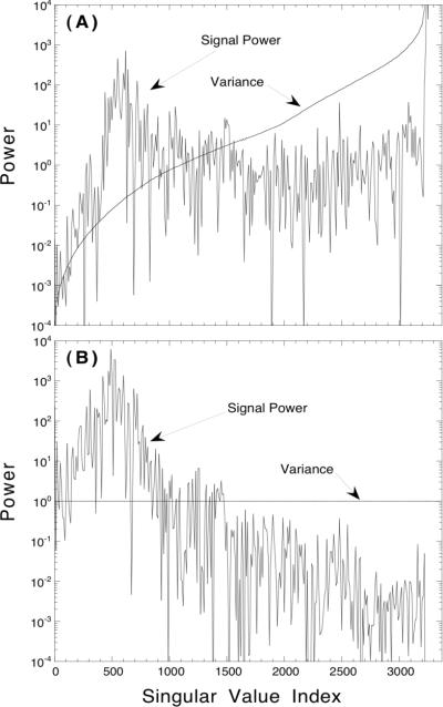
Sample plots of the signal power and variance spectra for an elliptical phantom are provided in Figure 1. These data are for a 20% wide photopeak energy window using RBSC, and the spectra are shown in both the image space (right singular vector basis) and projection space (left singular vector basis). The shape of the signal power spectrum depends on the ordering of the singular values and how the object features are represented in the singular vector basis. The “noise-like” fluctuations of the signal power spectrum are not noise related. The spectra in both spaces demonstrate the relative magnitude of the signal power to the variance for the various image components. However, the image space variance spectrum varies over several orders of magnitude, whereas the projection space variance spectrum is relatively flat. Using the projection space variance spectrum allows for easier comparison with other variance spectra–it enhances relative differences between spectra.

Figure 1.

Semi-logarithmic plots of the signal power and variance spectra calculated in (A) the image space (right singular vector basis) and (B) the projection space (left singular vector basis). The data are for a 20% wide photopeak energy window using RBSC at a count level of 3×10⁵ total counts.

The elements of MSP^RSV are the signal powers of the image components along the direction of each of the singular vectors. The true signal power spectrum is dependent upon the object to be imaged and the count level of the projection data. However, measured signal power spectra may differ from the true signal power spectrum. For example, the elements of the signal power which are in the null space will not be represented by the measured signal power spectrum. Also, inconsistencies between the projection data and the models used to generate the transfer matrices will give rise to bias in the measured signal power spectrum. We have calculated MSP^RSV for each of the data acquisition and reconstruction methods studied in this paper. Errors in MSP^RSV were found to be small enough to have negligible effect upon the relative noise levels of the various methods. This is not surprising since many of the methods studied are idealized in that the primary and scatter components are know exactly. In addition, the investigation has been limited to the energy range for which the scatter model used is reasonably accurate. Hence the bias in the reconstructed image is very small for each of the methods. Since the variance spectra are each relative to (essentially) the same signal power, they describe the relative differences in signal-to-noise between methods. Since they do not affect our conclusions, no further signal power spectra will be presented in this paper.

3. Methods

In order to investigate the fundamental issues regarding the reconstructibility and noise properties of scattered photons in SPECT, we have applied the SVD-based analysis methods discussed in the previous section to a Monte Carlo simulated phantom experiment. The use of Monte Carlo simulations allowed us to perfectly differentiate between primary and scattered photons, which was critical to the investigation undertaken but could not be achieved using experimental methods. In this section we describe the simulation experiment in depth, followed by details regarding the acquisition, reconstruction, and SVD analysis methods.

3.1. The Phantom

The phantom used in the simulation experiment is shown in Figure 2, and consisted of a water-filled cylinder with elliptical (32 × 24 cm) cross-section and infinite axial extent. Three cold rods with diameters 2, 3 and 5 cm were placed in the phantom, which had a uniform background of Tc-99m activity. The use of such a phantom that is uniform in the axial direction allows us to account for the 3D contributions of scatter and detector response while only treating a single 2D slice of the data. The analytical form of the phantom was used for the Monte Carlo simulations, and a transaxial slice of the phantom was digitized into a 64 × 64 matrix (pixel size = 0.625 cm) for display and reconstruction purposes.

Figure 2.

The elliptical phantom activity image (left) and attenuation map (right). The phantom contains 3 cold rods, with diameters of 2, 3 and 5 cm, in a uniform background of Tc-99m activity.

3.2. Monte Carlo Simulations

The SIMIND Monte Carlo program (Ljungberg and Strand 1989) was used to simulate projection data for a SPECT scan consisting of 128 evenly spaced views over 360° and using a primary photon energy of 140 keV. The imaging system simulated a gamma camera equipped with a low energy high resolution (LEHR) parallel-hole collimator. The energy resolution of the simulated camera was 11% at 140 keV and varied as $1∕\sqrt{\text{energy}}$. The effects of attenuation and ten orders of scatter (including coherent scatter) were included in the simulation, but photon interactions within the collimator were not modeled. Both inter- and intra-slice scatter were included. Since the phantom was uniform in the axial direction, single-slice 2D reconstructions can be performed that include the 3D effects of inter-slice scatter and detector response blurring.

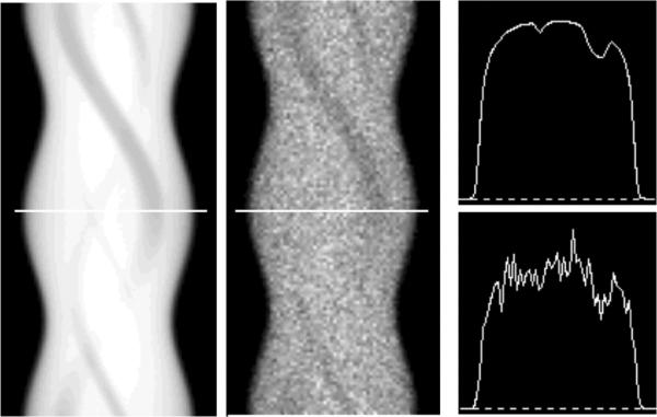
The projection data were simulated using 64 bins, each 0.625 cm wide. Primary data were stored separately from data which had undergone at least one scatter. A large number (8.7 × 10⁷) of photon histories were simulated at each viewing angle to obtain essentially noise-free data. The data were later scaled and Poisson noise was added to imitate a SPECT scan with 3 × 10⁵ total acquired counts in the 20% energy window. Figure 3 shows sinograms for a 20% wide photopeak energy window, demonstrating the noise-free quality of the simulated data relative to the noise level studied.

Figure 3.

Sinograms of the essentially noise-free Monte Carlo simulated projection data (left) and noisy projection data (center) at a count level of 3×10⁵ total counts. Horizontal profiles of the noise-free (top right) and noisy (bottom right) projection data are also shown.

3.3. Data Acquisition and Reconstruction Methods

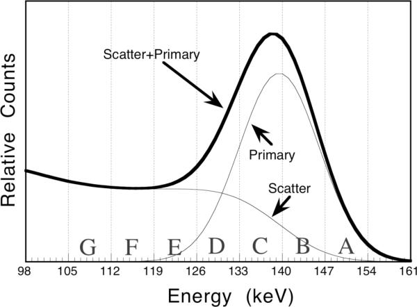
In this section we outline the energy window schemes and approaches to handling scatter that were studied in this paper. The measured energy spectrum of the simulated experiment is shown in Figure 4, where the components arising from primary and scattered photons are shown separately. A series of seven 7 keV wide energy windows have been defined over the energy range of 105– 154 keV and labeled by the letters A – G as shown in the figure. The energy windows used in this paper were all formed by combining windows A – G in various ways, and the labels of the inclusive windows will be used to describe each data set. For example, a single 20% wide energy window centered on 140 keV would accept photons from 126 – 154 keV, and is defined by the label ABCD. Multiple window projection data sets are designated by their constituent windows separated by commas. For example ABCD, EFG refers to a projection data set consisting of two windows: ABCD and EFG. Treatment of the multiple energy window data is discussed further in the following sections.

Figure 4.

Histogram of the measured energy spectrum indicating the components arising from scattered and primary photons. The series of 7 keV wide energy windows used in this study are indicated on the figure by the labels A – G.

Reconstruction-based scatter compensation was implemented using a number of energy window schemes. The RBSC methods were then compared with other, idealized approaches to handling scatter: Perfect Scatter Rejection, Ideal Scatter Subtraction, and Perfect Scatter Discrimination. For Perfect Scatter Rejection, only primary photons are acquired and reconstructed. In Ideal Scatter Subtraction, both primary and scattered photons are acquired, but the mean (noise-free) scatter component is subtracted prior to reconstruction. Perfect Scatter Discrimination is a new method in which primary and scattered photons are tagged and separated at acquisition. The resulting pair of data sets are then reconstructed simultaneously (modeling the SRF for the scatter-only data) to form a single image.

Perfect Scatter Rejection and Perfect Scatter Discrimination are the limiting cases in which it is assumed each photon can be tagged as either scattered or primary at acquisition. This would be realizable only for a detector with perfect energy resolution. Likewise, Ideal Scatter Subtraction is the limiting case in which the true mean scatter component is subtracted from the noisy projection data. This case would also be unrealizable in practice because the true scatter component is not known. Rather, it must be estimated using various methods and, as a result, is both biased and noisy. It is useful to study these idealized methods because they represent the upper limit for each approach for handling scatter. In contrast, the RBSC methods are not idealized since the scatter models used were not perfectly consistent with the Monte Carlo simulated data. Inaccuracies in the scatter models would lead to bias in the reconstructed images, an important effect in considering practical implementations of RBSC. The bias in the variance spectra arising from the model inaccuracies was found to be small enough to have negligible effect upon the conclusions of this paper. Comparing the (non-idealized) RBSC methods with other, idealized methods holds RBSC to a very high standard.

3.4. Transfer Matrices

To obtain accurate results, the effects of attenuation, detector response and scatter needed to be included in the calculation of the transfer matrices. While this can be done very accurately using Monte Carlo simulation (Floyd et al 1985a, Bowsher and Floyd 1991, Smith et al 1992a), it can be very computationally expensive, especially to obtain low noise results along the long scatter tails. For this reason we have chosen to generate the transfer matrices using a projector which models the effects of attenuation, detector response and scatter. The slab-derived scatter estimation (SDSE) model was used (Frey and Tsui 1993, Frey et al 1993a). Beekman et al (1993) have independently developed an essentially identical scatter model. The model is based on parametrizing the SRF for point sources placed in a large uniformly attenuating slab and has the advantage of not requiring any arbitrary parameters. It takes into account the shape of the scattering medium and position of the source to estimate the asymmetric, spatially variant SRF. The SDSE model has been shown to work very well in photopeak energy windows for uniformly attenuating objects and works moderately well for non-uniformly attenuating objects (Frey and Tsui 1994). However, assumptions are made which are not valid for low energies windows, and the scatter model exhibits some loss of accuracy at these energies. We have limited this investigation to the energy range for which the SDSE model is reasonably accurate. A new scatter model is currently being developed in our laboratory which should be more accurate for nonuniform attenuators and large angle scattering, and this model will allow lower energies to be included in the future.

Once the transfer matrices were generated, the corresponding design matrices (ΨF) were formed using weights from the essentially noise-free Monte Carlo projection data as described in the theory section. For the cases with multiple energy windows, each window was treated as an additional set of equations describing the source distribution. Hence the transfer matrices were larger for these cases.

3.5. Singular Value Decompositions

Once the design matrices were calculated, they were squared and the resulting products (F^TΨ⁻¹F) were decomposed using SVD. The SVDs were performed on a Cray T916 using the LAPACK routine SGESVD (Anderson et al 1990). All calculations were performed using Cray single precision (64-bit floating point). The singular values for each design matrix were then analyzed, and the signal power and variance spectra were computed. The SVD results were also used to compute the W-GMI reconstructed images and analytically calculated variance images for each method.

4. Results

4.1. Reconstructibility of Scattered Photons Near the Photopeak

Figure 5 shows the total response function for a line source placed off-center in the elliptical phantom for the 20% wide photopeak energy window. The components of the response due to primary and scattered photons are also shown. While the SRF is much broader than the primary photon response function, it still contains a peaked component. This indicates that scatter does contain some spatial information about the source activity distribution. To assess the quality of this information and study how it affects the reconstruction problem, we have decomposed the primary-only, scatter-only, and primary-plus-scatter design matrices using SVD. The resultant singular value spectra are shown in Figure 6. Each case had 8 zero singular values, but all the singular values beyond index 3228 were found to be so small as to be dominated by roundoff error. Thus we determined each matrix had rank 3228 and an effective nullity of 143. The presence of the null space is due to insufficient angular sampling and is typical for SPECT scans using an insufficient number of views.

Figure 5.

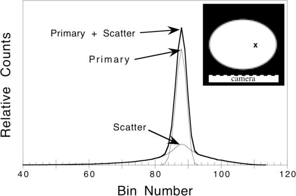
The total line source response function for a 20% wide energy window centered on the photopeak. The components of the response due to primary and scattered photons are indicated. The data are for a line source placed off-center in the elliptical phantom (inset).

Figure 6.

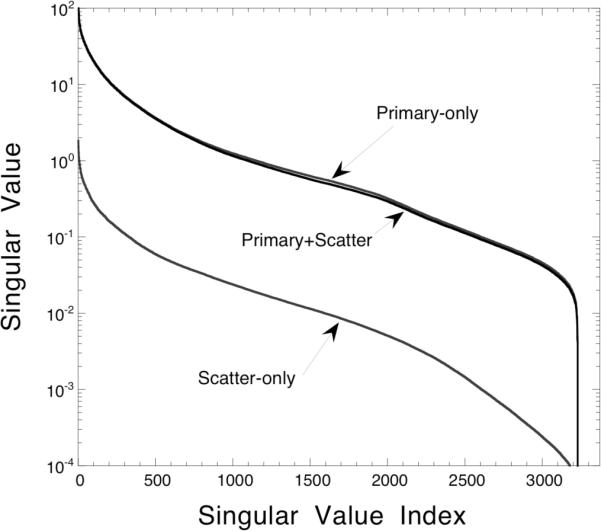
Singular value spectra for the primary-only, scatter-only, and primary plus scatter data using the 20% wide photopeak energy window. The vertical axis has been displayed using a logarithmic scale.

Since the primary-only, scatter-only, and primary-plus-scatter design matrices have the same ranks and nullities, the dimensions of the ranges and null spaces are the same for these matrices. It would be interesting to determine whether or not the actual ranges of each matrix coincide. If the primary-only and scatter-only design matrices have identical ranges, then the scatter-only data contains sufficient information to reconstruct the same image features as the primary data.

The right singular vectors corresponding to the zero singular values form a basis for the null space of each matrix. The degree of overlap between the ranges and null spaces of the matrices can be determined by computing the matrix product ${\mathbf{V}}_{\mathrm{p}}^{\mathbf{T}}{\mathbf{V}}_{\mathrm{s}}$, where V_p and V_s are the right singular vectors of the primary and scattered photon design matrices, respectively. Each element of ${\mathbf{V}}_{\mathrm{p}}^{\mathbf{T}}{\mathbf{V}}_{\mathrm{s}}$ is the dot product of the corresponding primary and scattered photon singular vectors. The matrix product ${\mathbf{V}}_{\mathrm{p}}^{\mathbf{T}}{\mathbf{V}}_{\mathrm{s}}$ can be broken into four regions (Figure 7) which contain the image components which are (I) common to the ranges of both matrices, (II) common to the null spaces of both matrices, and (III,IV) contained within the range of one matrix but the null space of the other. The sum of the squares of the ${\mathbf{V}}_{\mathrm{p}}^{\mathbf{T}}{\mathbf{V}}_{\mathrm{s}}$ elements in regions III and IV were found to be zero (up to the numerical accuracy of the computer used), indicating there was no crossover between the range of the primary photon design matrix and the null space of the scattered photon design matrix. This demonstrates that, not only does each matrix have the same rank and nullity, but the ranges and null spaces are also identical. In other words, if accurate scatter models are used and the data are consistent, then the scattered photon data theoretically contain sufficient information to reconstruct the exact same image as can be reconstructed from the primary photons. However, as can be seen from the singular value spectra, the scatter-only design matrix is poorly conditioned, indicating reconstructions from scatter-only projection data will be very sensitive to noise and other errors.

Figure 7.

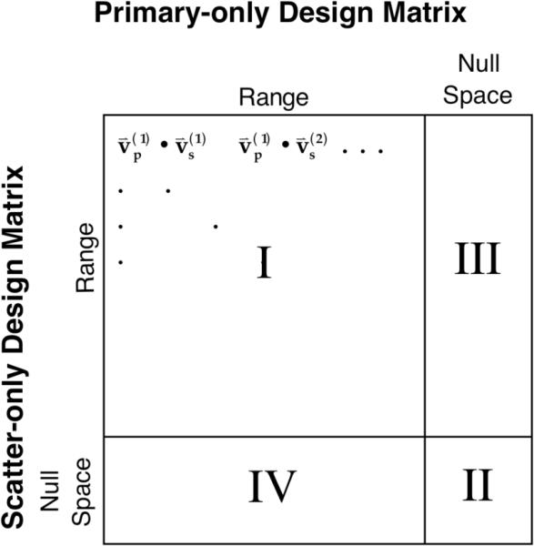
Diagram of the matrix product ${\mathbf{V}}_{\mathrm{p}}^{\mathbf{T}}{\mathbf{V}}_{\mathrm{s}}$ and the regions: (I) image components which are common to the range of both design matrices, (II) common null space image components, and (III,IV) image components which are in the range of one design matrix but the null space of the other.

We have reconstructed the noise-free primary-only and scatter-only projection data using the W-GMI reconstruction method. The images were regularized by truncating the singular value spectra at various indices, and the results are shown in Figures 8 and 9. Several observations can be made about these images. First, none of the scatter-only images accurately recover high frequency information about the phantom. This can be attributed to the ill-conditioning of the scatter-only design matrix. That matrix is so poorly conditioned that errors such as the small amount of noise in the “noise-free” simulation, slight inaccuracies in the scatter model and numerical error in the calculations are magnified drastically. While these effects are not substantial when using better-conditioned design matrices, the scatter-only design matrix is so poorly conditioned that these small inconsistencies in the data become important. To further demonstrate this, we have generated and reconstructed a noise-free and consistent data set (as opposed to using the Monte Carlo simulated data) using the transfer matrix and phantom image. The reader familiar with SVD will note that mathematically this amounts to little more than regularizing the phantom image by limiting the number of singular vectors used to represent the image. The resultant images are shown in Figure 10. The differences in the images of Figures 9 and 10 demonstrate the effects that small inconsistencies in the Monte Carlo data and numerical error can have when reconstructing with an ill-conditioned transfer matrix.

Figure 8.

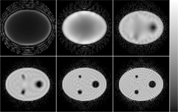
Noise-free W-GMI reconstructions of the primary-only data (Perfect Scatter Rejection). The images were regularized by truncating the singular value spectrum at: (top row, left to right) 500, 1000, 1500; (bottom row) 2000, 2500 and 3000 singular values.

Figure 9.

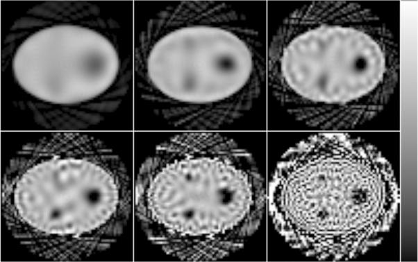
Noise-free W-GMI reconstructed images for the Monte Carlo scatter-only projection data in the 20% wide photopeak energy window. The images were regularized by truncating the singular value spectrum at: (top row, left to right) 100, 250, 400; (bottom row) 500, 750 and 1500 singular values.

Figure 10.

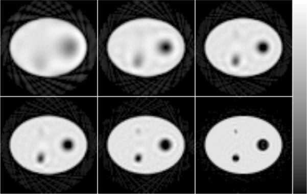
Noise-free W-GMI images reconstructed from consistent (model-generated) scatter-only projection data in the 20% wide photopeak energy window. The images are ordered in the same way as in Figure 9, and indicate the image quality obtainable from consistent, noise-free data and minimal numerical error.

Second, the images of Figures 8 and 9 have very different characteristics at the various degrees of regularization shown. Recall the early singular value indices correspond to image components which are less sensitive to noise, and the latter indices correspond to image components which are more sensitive to noise. These images indicate that, when using the primary photon data, high frequency information near the phantom surface is recovered more easily than lower frequency information at greater depths. For the scatter-only data all high frequency information tends to be more difficult to recover. The reason is that the shallow peak and broad tails of the SRF tend to blur any high frequency features.

The results of this section indicate that scatter-only projection data does contain reconstructible information about the source activity distribution, but this information is very poorly conditioned. Reconstruction from scatter-only projection data is therefore possible, but unlikely to provide any benefit because such reconstructions will be very sensitive to noise and inaccuracies in the scatter models used. However, this result does suggest that scattered photons might be useful when used in conjunction with primary photons. This premise is investigated further in the following sections.

4.2. Evaluation of Photopeak Window Methods

We have shown that scattered photons with energies near the emission peak contain useful, though poorly conditioned, information about the source distribution. We turn now to investigating approaches to handling scatter in photopeak energy windows (Table I), and we analyze the noise levels of each of these methods. The variance spectra for each of the photopeak window methods studied are shown in Figure 11. Perfect Scatter Discrimination was found to result in the lowest variance, followed closely by Perfect Scatter Rejection. The 20% Window RBSC method outperformed Ideal Scatter Subtraction, but performed worse than Perfect Scatter Rejection. This indicates that, if scattered counts are combined with primaries as in the 20% Window RBSC method, then the scattered counts have the effect of increasing the variance of the reconstructed image. This is because the presence of scattered photons results in a degraded response function (less peaked and longer tails than the primary-only response function), hence the corresponding design matrix is more poorly conditioned. However, if the scattered photons are separated from the primaries (as in Perfect Scatter Discrimination), then no such degradation occurs and the scattered data can be used to reduce the variance. Instead of degrading the primary-only response function, the tagged scattered photons provide an additional data set which can be used in a productive manner. Of course, Perfect Scatter Discrimination is unrealizable in practice. However, this result indicates that discarding scattered photons might not be the best approach, even if gamma cameras are developed in the future which have better scatter discrimination capabilities.

Table I.

Description of the methods studied which use only data in a 20% wide energy window centered on the 140 keV photopeak.

Name	Description
Ideal Scatter Subtraction	The true mean (noise-free) scatter component is subtracted prior to reconstruction
20% Window RBSC	The SRF is modeled during the reconstruction
Perfect Scatter Rejection	Only primary photons are acquired and reconstructed
Perfect Scatter Discrimination	Two data sets are acquired—one containing only primary photons, the other only scattered photons—and both data sets are reconstructed simulataneously

Figure 11.

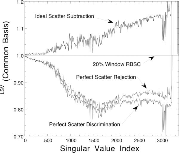
Variance spectra for each of the methods that use only photons from a 20% wide photopeak energy window. The spectra have been expressed using the common basis formed by the left singular vectors of the 20% Window RBSC design matrix.

4.3. Reconstructibility of Lower Energy Scattered Photons

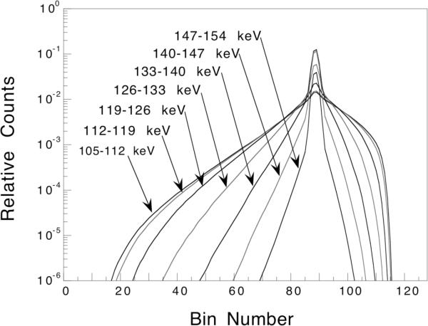
We have shown that scattered photons with energies near the photopeak can be used in the reconstruction to gain some reduction in variance. The question that follows, then, is whether or not lower energy scattered photons can also be used for the same purpose. Figure 12 shows the total response function for a line source placed in our phantom for each of the 7 keV wide energy windows A – F. The response function becomes broader for lower energies because fewer primary and more scattered photons are included. Also, at the lower energies there are more large angle and multiple scatters, which results in a SRF which is both broader and more difficult to model.

Figure 12.

Total line source response functions for the 7 keV wide energy windows A – G. The data are for a line source placed off-center in the elliptical phantom, and the vertical axis has been displayed using a logarithmic scale. The profiles are not normalized, so the relative number of counts in each window can be assessed from the figure.

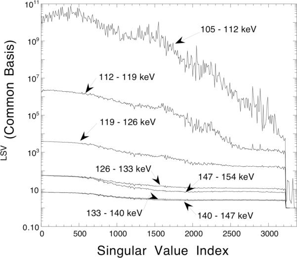
To assess the quality of information in these windows, we have computed design matrices for each and decomposed them using SVD. The resultant singular value spectra are shown in Figure 13, and the corresponding variance spectra are shown in Figure 14. Again we found that the ranges (and null spaces) for each window were essentially identical. The design matrices for the lower energy windows, which contain mostly multiple or wide angle scattered photons, were very poorly conditioned. They resulted in variance spectra which were several orders of magnitude higher than for the windows near the photopeak, even though the number of counts in each window were on the same order of magnitude. The investigation was stopped at 105 keV for two reasons. First, the scattered photon design matrices were becoming very poorly conditioned at these energies; and, second, this was the lower limit of the energy range for which the SDSE scatter model was reasonably accurate.

Figure 13.

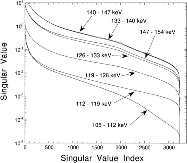
Singular value spectra for each of the 7 keV wide energy windows A–G. The vertical axis has been displayed using a logarithmic scale.

Figure 14.

Variance spectra, expressed using the common basis, for each of the 7 keV wide energy windows A–G. The vertical axis has been displayed using a logarithmic scale.

4.4. Evaluation of Methods Including Lower Energy Scattered Photons

A number of methods were studied that use low energy photons in addition to photopeak window data (Table II). Several energy window schemes were studied using RBSC; and for the other approaches to handling scatter, data from the entire energy range of 105–154 keV was included (when applicable). The resultant variance spectra are shown in Figure 15, where the 20% Window RBSC method has been included for comparison.

Table II.

Description of the energy windows and methods studied which include low energy photons. Each of the methods use RBSC except for Perfect Scatter Rejection, and the 20% Window RBSC method is included for comparison. The labels used for the energy windows are defined in Figure 4, and multiple windows are designated by separating the labels by commas.

Name	Energy Windows	Description
20% Window RBSC	ABCD	20% wide photopeak window
49 keV Window RBSC	ABCDEFG	Single, wide energy window
Contiguous Windows RBSC	A, B, C, D, E, F, G	Seven small energy windows
Dual Window RBSC	ABCD, EFG	20% wide photopeak window and a secondary scatter window
Perfect Scatter Rejection	ABCDEFG primary-only	Only primary photons are acquired and reconstructed
Perfect Scatter Discrimination	ABCDEFG primary-only, ABCDEFG scatter-only	Separate primaries from scatter and reconstruct simultaneously, using RBSC for the scattered data

Figure 15.

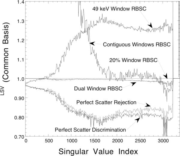
Plots of the variance spectra for the cases which used low energy photons in addition to photopeak data. The 20% Window RBSC case is included for comparison, and all spectra have been expressed using the photopeak window left singular vectors as a common basis.

When performing RBSC, using a single 49 keV wide energy window resulted in a relatively low variance for the earliest image components (representing low frequency, shallow depth information), but the latter image components had a relatively high variance. The opposite effect was seen when using a large number of smaller windows (Contiguous Windows RBSC method). Dual Window RBSC performed the best of the practical methods, resulting in a variance spectrum that was slightly lower than that for the 20% Window RBSC method. This case approximates perfect scatter discrimination—the photopeak window contains mostly primary counts, and the lower energy window contains primarily scatter. The large differences between the RBSC spectra demonstrate the importance of choosing the correct energy window scheme when low energy scattered photons are included in the data. In practice, the use of multiple energy windows carries a significant computational cost, and this must be weighed against the benefits of including low energy data.

Of the idealized approaches to handling scatter, Perfect Scatter Discrimination again resulted in the lowest variance, outperforming Perfect Scatter Rejection. However, the inclusion of low energy scattered photons led to only small improvements as compared to using only photons near the photopeak (compare the Perfect Scatter Discrimination curves of Figures 11 and 15). Again, we see that scattered photons can be included in the reconstruction to reduce image noise; but the poor conditioning of the scattered photon design matrix means that only a slight reduction in variance can be obtained.

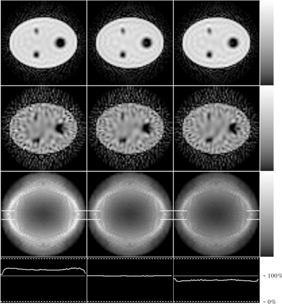
Figure 16 shows noisy and noise-free W-GMI reconstructions and variance images for three of the methods: 49 keV Window RBSC, Dual Window RBSC, and Perfect Scatter Discrimination. These three cases form a representative set containing a poor choice of energy windows (49 keV Window RBSC), the best practically achievable method studied (Dual Window RBSC), and the best idealized method studied (Perfect Scatter Discrimination). The images were regularized by truncating the singular value spectrum at index 2000. The noise-free images (top row) are very similar for each of these methods, and indicate that, in the absence of noise, each of these methods provides nearly the same reconstructed images. This result is in agreement with the SVD analysis. The images reconstructed from noisy data (middle row) show some differences in noise texture and extent, and these differences in noise levels are demonstrate more dramatically by the variance images and relative profiles (bottom two rows).

Figure 16.

Images for 49 keV Window RBSC (left), Dual Window RBSC (center), and Perfect Scatter Discrimination (right): noise-free data (top row), noisy data (second row), and variance images (third row). Horizontal profiles (bottom row) show the relative heights of these variance images (thick lines) relative to the “standard” 20% Window RBSC variance image (thin line). They were obtained by dividing these variance images by that for the 20% Window RBSC method, and then taking profiles across the resultant “relative” variance images. All images were regularized by including 2000 singular values in the W-GMI reconstruction, and the images of each row are displayed using the greyscales shown at the right.

The variance images were divided by the variance image for the 20% Window RBSC method (not shown), and horizontal profiles were drawn across the resultant “relative” variance images (bottom row of the figure). The differences in the variance images agree with the variance spectra results presented earlier. The average variance across the phantom for the 49 keV Window RBSC method was 24% higher than that for the 20% Window RBSC method, and Dual Window RBSC and Perfect Scatter Discrimination resulted in variance reductions of 1% and 18%, respectively. When more singular values were included in the reconstruction, greater differences between the methods were observed. These results demonstrate that the variance spectra correlate with the variance of W-GMI reconstructed images.

5. Discussion

The results shown in the preceding sections were all for count levels corresponding to 3 × 10⁵ total counts in the 20% wide photopeak window. We repeated the analysis for each of the key methods at three other count levels: 0.75 × 10⁵, 1 . 5 × 10⁵ and 6 × 10⁵ total counts in the 20% photopeak window. No substantial differences in relative noise levels were observed, and the conclusions drawn in this paper are valid throughout this range of count levels.

It is important to keep in mind the limitations of this study. We have focused upon reconstructed image noise levels, making comparisons valid across a wide range of regularizations. In order to implement a scatter compensation scheme, it is important to account for a number of other factors, such as computational requirements of the reconstruction, potential bias resulting from inaccuracies in the scatter models or estimates, capability of multiple-energy window acquisition, and so on. This work is intended to guide future research in handling scatter in SPECT. One difference between this paper and earlier work (Kadrmas et al 1996) is that the statistics of the problem were modeled more accurately by including statistical weights in the SVD analysis. This had the most effect upon the performance of RBSC methods which use multiple energy windows, and we found that using a pair of windows was better than using a large number of smaller windows.

One of the things that we have not addressed in this paper is what happens below 105 keV. For example, there may be an improvement in the quality of the scattered data as we approach 90 keV. This is the energy of the backscatter peak, which contains many photons that have been emitted in a direction away from the detector and undergone a single scatter through 180°. The result is a response function for backscattered photons which is similar to that for primary photons, but blurred by the collimator response function at the depths at which the backscatter occurs. The SRF near 90 keV will consist of a component due to backscattered photons in addition to components arising from multiply scattered photons. It is likely the design matrix for a backscatter energy window would be better conditioned than for other, low energy scatter windows, and inclusion of such data might be a fruitful area for future study.

On a similar note, energy windows near 70–90 keV will contain a large number of counts arising from lead fluorescence x-rays produced within the collimator. The spatial distribution of these x-rays contains both primary-like and scatter-like components (Moore et al 1995). It may be possible to model the distribution of fluorescence x-rays in a manner similar to RBSC. Since there is a primary-like component, using an x-ray energy window in addition to photopeak windows may result in further reductions in reconstructed image variance.

6. Summary and Conclusions

This study addressed some of the fundamental issues regarding the phenomenon of photon scatter in SPECT. We have analyzed the reconstructibility of scattered photons in Tc-99m SPECT and investigated methods of using scattered counts to reduce the noise levels of reconstructed images. Techniques based upon the SVD of the system design matrix were used to determine the range and null space of systems which reconstruct scattered projection data through the use of scatter models. The analysis was performed for energies as low as 105 keV. In all cases it was found that the ranges (and null spaces) for the scatter-only and primary-only design matrices coincided exactly. In other words, the scattered photon projection data theoretically contain sufficient information to reconstruct, in the absence of noise, the exact same image as primary photons. However, the scattered photon design matrices were found to be poorly conditioned, and hence very sensitive to noise. This condition was found to worsen at lower energies.

In terms of utilizing scattered photons to reduce image noise, we have compared a variety of methods which model the scatter response function during the reconstruction (reconstruction-based scatter compensation). To accomplish this, we used analysis techniques based upon the SVD of the system design matrix. These techniques provide information for a wide range of regularizations, and allow us to draw conclusions which are essentially regularization-independent. Systems using both single and multiple energy windows were studied, and it was found that the noise properties of the various image components were dependent upon the energy windows used. In all cases it was found that more than one energy window was required if low energy photons were to be included to reduce variance.

Reconstruction-based scatter compensation was also compared to other, idealized methods of handling scatter. Lower noise levels were achieved with RBSC than with Ideal Scatter Subtraction, but both fared worse than if all scattered photons could be rejected outright at acquisition (Perfect Scatter Rejection). However, if it were possible to tag and separate the primary and scattered components at acquisition, then the resulting pair of data sets could be reconstructed using RBSC to obtain the lowest noise levels (Perfect Scatter Discrimination). Of course, perfect discrimination of scattered events from primaries cannot be achieved in practice. However, this case does indicate that outright rejection of scattered photons may not be the best approach.

The best achievable method studied was Dual Window RBSC, which employed a photopeak window and a secondary scatter window. This approximates Perfect Scatter Discrimination: the upper window accepts mostly unscattered events, whereas the lower window contains primarily scatter. It was found that Dual Window RBSC provided some reduction in variance as compared to using a single photopeak window, but it did not approach the limiting case of Perfect Scatter Discrimination. This is evidence that improvements in the scatter discrimination capabilities of gamma cameras could lead to reductions in the noise levels of reconstructed images. Since RBSC outperformed the idealized limit on subtraction-based scatter compensation, it is deemed worthwhile for researchers to continue working to bring RBSC to the clinic. The results of this study indicate that scattered photons can be utilized through RBSC to achieve some reductions in the noise levels of Tc-99m SPECT images. However, the energy window scheme must chosen carefully to ensure that the scattered photon counts are used productively.

References

- Anderson E, Bai Z, Bischof C, Demmel JW, Dongarra JJ, Du Croz J, Greenbaum A, Hammarling S, McKenney A, Sorenson D. Computer Science Dept. Technical Report CS-90-105. University of Tennessee; Knoxville: 1990. LAPACK: A portable linear algebra library for high-performance computers. [Google Scholar]
- Axelsson B, Msaki P, Israelsson A. Subtraction of Compton-scattered photons in single-photon emission computerized tomography. J. Nucl. Med. 1984;25:490–494. [PubMed] [Google Scholar]
- Beekman FJ, Eijkman EGJ, Viergever MA, Borm GF, Slijpen ETP. Object shape dependent PSF model for SPECT imaging. IEEE Trans. Nucl. Sci. 1993;NS-40:31–39. [Google Scholar]
- Bowsher JE, Floyd CE. Treatment of Compton scattering in maximum-likelihood, expectation-maximization reconstructions of SPECT images. J. Nucl. Med. 1991;32:1285–91. [PubMed] [Google Scholar]
- Floyd CE, Jaszczak RJ, Coleman RE. Inverse Monte Carlo: a unified reconstruction algorithm. IEEE Trans. Nucl. Sci. 1985a;NS-32:779–785. [PubMed] [Google Scholar]
- Floyd CE, Jaszczak RJ, Greer KL, Coleman CE. Deconvolution of Compton scatter in SPECT. J. Nucl. Med. 1985b;26:403–8. [PubMed] [Google Scholar]
- Floyd CE, Jaszczak RJ, Harris CC, Coleman RE. Energy and spatial distribution of multiple order Compton scatter in SPECT: a Monte Carlo investigation. Phys. Med. Bio. 1984;29:1217–30. doi: 10.1088/0031-9155/29/10/005. [DOI] [PubMed] [Google Scholar]
- Frey EC, Ju Z-W, Tsui BMW. A fast projector-backprojector pair modeling the asymmetric, spatially varying scatter response function for scatter compensation in SPECT imaging. IEEE Trans. Nucl. Sci. 1993a;NS-40:1192–1197. [Google Scholar]
- Frey EC, Tsui BMW. Spatial properties of the scatter response function in SPECT. IEEE Trans. Nucl. Sci. 1991;NS-38:789–794. [Google Scholar]
- Frey EC, Tsui BMW. A practical method for incorporating scatter in a projector-backprojector for accurate scatter compensation in SPECT. IEEE Trans. Nucl. Sci. 1993;NS-40:1107–1116. [Google Scholar]
- Frey EC, Tsui BMW. Modeling the scatter response function in inhomogenous scattering media for SPECT. IEEE Trans. nucl. Sci. 1994;NS-41:1585–93. [Google Scholar]
- Frey EC, Tsui BMW, King MA, Ljungberg M. A quantitative comparison of extended dual photon window and iterative reconstruction based scatter compensation. J. Nucl. Med. 1993b;34:72. [Google Scholar]
- Frey EC, Tsui BMW, Ljungberg M. Conference Record of the 1992 IEEE Medical Imaging Conference. 1992. A comparison of scatter compensation methods in SPECT: subtraction-based techniques versus iterative reconstruction with accurate modeling of the scatter response; pp. 1035–37. [Google Scholar]
- Gagnon D, Todd-Pokropek A, Arsenault A, Dupras G. Introduction to holospectral imaging in nuclear medicine for scatter subtraction. IEEE Trans. Med. Imag. 1989;MI-8:245–50. doi: 10.1109/42.34713. [DOI] [PubMed] [Google Scholar]
- Gilardi MC, Bettinardi V, Todd-Pokropek A, Milanesi L, Fazio F. Assessment and comparison of three scatter correction techniques in single photon emission computed tomography. J Nucl. Med. 1988;29:1971–79. [PubMed] [Google Scholar]
- Golub GH, Loan CFV. Matrix Computations. John Hopkins University Press; Baltimore: 1989. [Google Scholar]
- Gullberg GT, Huesman RH, Zeng GL, Foresti SA. Conference Record of the 1995 IEEE Medical Imaging Conference. 1995. Efficient estimation of dynamic cardiac SPECT kinetic parameters using weighted least squares estimation of dynamic reconstructions; pp. 1684–88. [Google Scholar]
- Gullberg GT, Zeng GL. A reconstruction algorithm using singular value decomposition of a discrete representation of the exponential radon transform using natural pixels. IEEE Trans. Nucl. Sci. 1994;NS-41:2812–19. [Google Scholar]
- Hamill JJ, Devito RP. Scatter reduction with energy-weighted acquisition. IEEE Trans. Nucl. Sci. 1989;NS-36 [Google Scholar]
- Huesman RH, Gullberg GT, Greenberg GL, Budinger TF. Lawrence Berkeley Lab. Publ. PUB-214. 1977. Donner Algorithms for Reconstruction Tomography. [Google Scholar]
- Jaszczak RJ, Greer KL, Floyd CE, Harris CC, Coleman RE. Improved SPECT quantitation using compensation for scattered photons. J. Nucl. Med. 1984;25:893–900. [PubMed] [Google Scholar]
- Kadrmas DJ, Frey EC, Tsui BMW. An SVD investigation of modeling scatter in multiple energy windows for improved SPECT imaging. IEEE Trans. Nucl. Sci. 1996;43:2275–84. doi: 10.1109/23.531892. [DOI] [PMC free article] [PubMed] [Google Scholar]
- King MA, Hademenos GJ, Glick SJ. A dual-photopeak window method for scatter correction. J. Nucl. Med. 1992;33:605–612. [PubMed] [Google Scholar]
- Koral KF, Wang X, Rogers WL, Clinthorne NH, Wang X. SPECT Compton-scattering correction by analysis of energy spectra. J. Nucl. Med. 1988;29:195–202. [PubMed] [Google Scholar]
- Ljungberg M, King MA, Hademenos GJ, Strand S-E. Comparison of four scatter correction methods using Monte Carlo simulated source distributions. J. Nucl. Med. 1994;35:143–51. [PubMed] [Google Scholar]
- Ljungberg M, Msaki P, Strand S-E. Comparison of dual-window and convolution scatter correction techniques using the Monte Carlo method. Phys. Med. Biol. 1990;35:1099–1110. [Google Scholar]
- Ljungberg M, Strand S-E. A Monte Carlo program for the simulation of scintillation camera characteristics. Comp. Meth. Prog. Biomed. 1989;29:257–272. doi: 10.1016/0169-2607(89)90111-9. [DOI] [PubMed] [Google Scholar]
- Msaki P, Axelsson B, Dahl CM, Larsson SA. Generalized scatter correction method in SPECT using point scatter distribution functions. J. Nucl. Med. 1987;28:1861–69. [PubMed] [Google Scholar]
- Moore SC, English RJ, Syravanh C, Tow DE, Zimmerman RE, Chan KH, Kijewski MF. Simultaneous Tc-99m/Tl-201 imaging using energy-based estimation of the spatial distribution of contaminant photons. IEEE Trans. Nucl. Sci. 1995;42:1189–95. [Google Scholar]
- Ogawa K, Harata Y, Ichihara T, Kubo A, Hashimoto S. A practical method for position-dependent Compton scatter correction in single photon CT. IEEE Trans. Med. Imag. 1991;MI-10:408–12. doi: 10.1109/42.97591. [DOI] [PubMed] [Google Scholar]
- Press WH, et al. Numerical Recipes in C. Cambridge University Press; Cambridge: 1988. [Google Scholar]
- Pretorious PH, van Rensburg AJ, van Aswegen A, Lotter MG, Serfontein DE, Herbst CP. The channel ratio method of scatter correction for radionuclide image quantitation. J. Nucl. Med. 1993;34:330–35. [PubMed] [Google Scholar]
- Smith MF, Floyd CE, Jaszczak RJ, Coleman RE. Reconstruction of SPECT images using generalized matrix inverses. IEEE Trans. Med. Imag. 1992a;MI-11:165–175. doi: 10.1109/42.141640. [DOI] [PubMed] [Google Scholar]
- Smith MF, Jaszczak RJ, Coleman RE. Conference Record of the 1992 IEEE Medical Imaging Conference. 1992b. Simultaneously constraining SPECT activity estimates with primary and secondary energy window projection data; pp. 1175–77. [DOI] [PubMed] [Google Scholar]
- Welch A, Gullberg GT, Christian PE, Datz FL. A transmission-map-based scatter correction technique for SPECT in inhomogenous media. Med. Phys. 1995;22:1627–35. doi: 10.1118/1.597422. [DOI] [PubMed] [Google Scholar]
- Yanch JC, Flower MA, Webb S. A comparison of deconvolution and windowed subtraction techniques for scatter compensation in SPECT. IEEE Trans. Med. Imag. 1988;MI-7:13–20. doi: 10.1109/42.3924. [DOI] [PubMed] [Google Scholar]