AUTOMATED ACTIN FILAMENT SEGMENTATION, TRACKING AND TIP ELONGATION MEASUREMENTS BASED ON OPEN ACTIVE CONTOUR MODELS

Abstract

This paper presents an automated method for actin filament segmentation and tracking for measuring tip elongation rates in Total Internal Reflection Fluorescence Microscopy (TIRFM) images. The main contributions of the paper are: (i) we use a novel open active contour model for filament segmentation and tracking, which is fast and robust against noise; (ii) different strategies are proposed to solve the filament intersection problem, which is shown to be the main difficulty in filament tracking; and (iii) this fully automated method avoids the need of human interaction and thus reduces required time for the entire elongation measurement process on an image sequence. Application to experimental results demonstrated the robustness and effectiveness of this method.

1. INTRODUCTION

The ability of actin proteins to self-assemble into long filaments of over 10 µm in length and ~7 nm in thickness is important for eukaryotic cells: actin filaments provide cells with mechanical integrity, generate forces for cell movement by polymerization, and act as tracks for intracellular transport by motor proteins. Total Internal Reflection Fluorescence Microscopy (TIRFM), is a technique that has be used widely to image the kinetics of polymerization of individual actin filaments growing on a glass surface in vitro [2, 3, 7].

The two ends of an actin filament (the “barbed” and “pointed” end, respectively) grow at different rates. Surface tethers act as pivot points that can be used as fiducial markers to help distinguish the elongation of each end [2, 3, 7]. Two basic features of actin kinetics that can be extracted from such images are (i) the average rate of filament elongation at each end, and (ii) the fluctuations in the average rate. Both of these two numbers depend in a unique way on the details of the microscopic mechanism of monomer addition to the ends of the filament [2, 3].

Measurement of filament elongation versus time in TIRFM images is typically performed using manual or semi-automated methods [2, 7]. The lack of fully automated image analysis methods to simultaneously measure multiple filaments limits the use of TIRFM as an efficient method to extract detailed statistics on filament elongation.

Tracking techniques on similar image data have been proposed. Hadjidemetriou et al. [4] developed a method to automatically track microtubules (MT) which are characterized locally using level sets of minimal paths. Smal et al. [10] utilized particle filters (PF) to track tips of polymerizing MTs. Kong et al. [6] employed a PF-based method similar to [10] to track MT tips. Open active contours were then used to segment MT bodies based on estimated tip locations. Saban et al. [9] automatically detected tips in the first frame and then proceeded to track each tip separately by searching for the closest match in subsequent frames.

In this paper, we report a novel and fully automated image analysis method for actin filament segmentation, tracking and tip elongation measurement in TIRFM images of actin polymerization in vitro. We use open active contour models which can stretch along the filament body to segment and track filaments. To solve the filament intersection problem, we propose two strategies, greater tip stiffness and tip “jump” strategies. In every frame, newly appeared filaments are detected. To accurately measure the tip elongation rate of filaments, contiguous frame registration is performed.

2. METHODOLOGY

2.1. Filament Segmentation

Conventional 2D segmentation methods such as active contour models (Snake) [5] are not straightforwardly applicable to this problem because of the following reasons. (i) Computed boundaries of intersected filaments are linked together and therefore cannot be distinguished as different filaments; (ii) The width of filaments in the images is only 2–4 pixels wide. Exact boundaries of filaments are not relevant to this problem, since we are interested in accurate measurement of filament length and its elongation rate.

We observe the appearance of bright ridges at the central line of each filament. Therefore, promising segmentation performance can be achieved by locating central lines of filaments with estimated filament width, which is constant. To locate those bright ridges, we propose a new active contour based segmentation and tracking method. However, unlike the conventional active contour algorithms which utilize closed curves as snakes, open curves are used instead.

Representing an open curve parametrically, r(s) = (x(s), y(s)), s ∈ [0, 1], the active contour works by minimizing its overall contour energy, E, which is composed of internal energy E_int and external energy E_ext, i.e. E = E_int + E_ext. The internal energy term, E_int, is defined similar to closed snakes:

$$E_{\mathit{\text{int}}}={\displaystyle {\int }_0^1(\alpha (s)|{\mathbf{r}}_s(s){|}^2+\beta (s)|{\mathbf{r}}_{ss}(s){|}^2)ds.}$$ (1)

More specifically, a first-order term that represents the “elasticity” energy of a snake and a second-order term that represents the “stiffness” energy of a snake are controlled by α(s) and β(s), respectively.

The external energy term consists of two terms: the image term E_img and the stretching term E_str:

$$E_{\mathit{\text{ext}}}={\displaystyle {\int }_0^{1}k·(E_{\mathit{\text{img}}}(\mathbf{r}(s))+k_{\mathit{\text{str}}}·E_{\mathit{\text{str}}}(\mathbf{r}(s)))ds,}$$ (2)

where k is a constant that balances the internal and external energy, and k_str is a constant that balances the image term and the stretching term, which are defined below.

2.1.1. Image Term

We directly use the Gaussian-filtered image E_img = G_σ *I as the image term, which is different from the gradient magnitude term |∇G_σ * I|² commonly used in conventional segmentation methods. Gradient vectors of ∇E_img point toward the center of filaments. In contrast, gradient vectors of ∇|∇G_σ * I|² point toward boundaries of filaments.

2.1.2. Stretching Term

As mentioned above, gradient vectors of ∇E_img point toward the center of filaments. To make a snake stretch along the filament, stretch forces are added to tips (s = 0 and 1) of a snake. The stretch forces point along tangent directions of the snake’s tips. The force magnitude is defined by F(r(s)) = (I(r(s)) − I_mean)/(I_f − I_b), where I (r(s)), I_f, I_b, and I_mean denote the pixel value covered by a certain point r(s) on the snake, the foreground (filament) intensity, the background intensity, and the mean of foreground and background intensity, respectively. The latter three parameters are constant and estimated beforehand. Consequently, the gradient fields of the stretching term is defined by

$$\nabla E_{\mathit{\text{str}}}(\mathbf{r}(s))=\{\begin{array}{cc}-\frac{{\mathbf{r}}_s(s)}{|{\mathbf{r}}_s(s)|}·F(\mathbf{r}(s))& s=0,\hfill \\ \frac{{\mathbf{r}}_s(s)}{|{\mathbf{r}}_s(s)|}·F(\mathbf{r}(s))& s=1,\hfill \\ 0& \mathit{\text{otherwise}}.\hfill \end{array}$$ (3)

2.1.3. Snake Dynamic Deformation

Summarizing all terms, the snake points at iteration i are calculated from model points at iteration i − 1 as follows:

$$x_i={(A+\gamma I)}^{-1}(\gamma x_{i-1}-\partial E_{\mathit{\text{ext}}}(x_{i-1},y_{i-1})/\partial x),$$ (4)

$$y_i={(A+\gamma I)}^{-1}(\gamma y_{i-1}-\partial E_{\mathit{\text{ext}}}(x_{i-1},y_{i-1})/\partial y),$$ (5)

where A is the pentadiagonal banded matrix that specifies the internal smoothness constraints of the model defined by Equation (1), matrix I is the identity matrix and γ is the step size [5]. Using the above optimization method, snakes can efficiently deform to desired filament central line locations.

2.2. Filament Tracking

Let I_t and r^k,t represent the tth frame of an image sequence and the kth snake in the tth frame, respectively. To initialize snakes in the tth frame, all n snakes in the t − 1th frame, r^1:n,t−1, are used. Newly appeared filaments are also detected and initialized as new snakes by utilizing the ridge detection in scale-space method [8] using a fixed scale σ.

Because all filaments are able to grow (polymerize) or shrink (depolymerize), snake deformation consists of two main steps. Firstly, we let a snake readjust to its corresponding filament by setting α(s) to a greater value and by letting ∇E_str(r(s)) = 0 for s ∈ [0, 1]. This means assigning greater “elasticity” energy but no stretching energy to the snake. By doing so, the snake shrinks as its body equilibrates along the bright ridge of its corresponding filament. Once all pixel values covered by the snake are greater than I_mean, the snake stops to shrink. Secondly, α(s) is set to a smaller value and E_str(r(s)) is set according to Equation 3. During the snake’s deformation process, if both ends of the snake grow less than a given threshold in one iteration, the snake is assumed to be converged.

2.2.1. Frame Drift

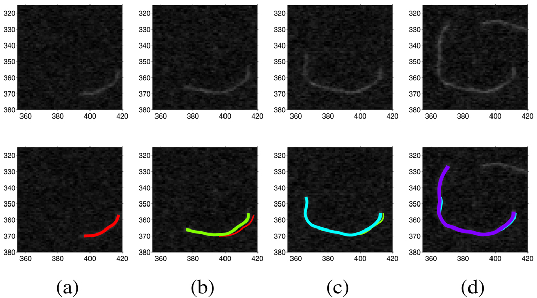
Image sequences obtained through TIRFM microscopy show drift, i.e., translation, between contiguous frames [7]. Because of the image term in the energy function, whose gradient vectors point toward center of filaments in a wide range, snakes are able to track their corresponding filaments during frame drift. In Figure 1, we illustrate the frame drift phenomenon and the performance of our method against frame drift. An obvious frame drift can be observed and our method successfully tracks the filament’s polymerizing and deploymerizing as well as its overall movement in the image plane.

Fig. 1.

Tracking a filament with drift between frames. (a) The 1st frame’s snake (red), (b) the 4th frame’s snake (green) and the 1st frame’s snake (red), (c) the 9th frame’s snake (cyan) and the 4th frame’s snake (green), and (d) the 13th frame’s snake (purple) and the 9th frame’s snake (cyan).

2.2.2. Filament Intersection

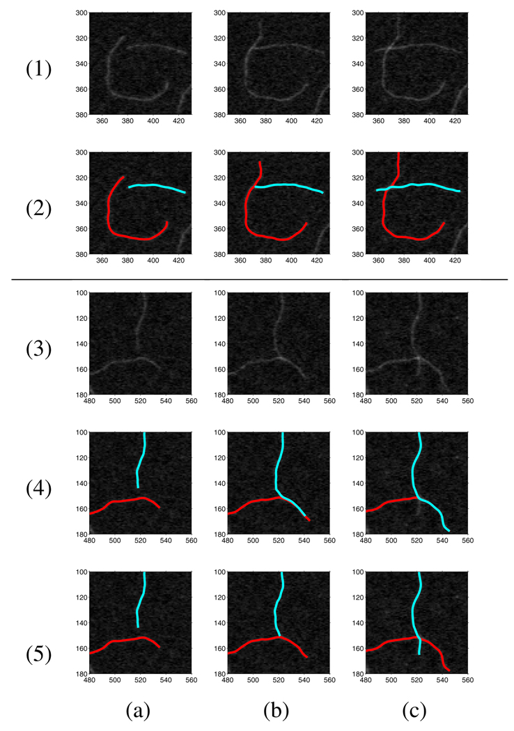
Filaments may intersect with each other during the tracking process. At an intersection of two filaments A and B, a snake tracking filament A may falsely extend along B. Several strategies are employed to let snakes have higher probability of tracking their corresponding filaments. A condition to predict filament intersection is when the distance between one of a snake’s outer tips and another snake is less than a given threshold, the predicted intersection point s′ on the latter snake is computed. A greater value is assigned to β(s) of the nearby tip of the former snake, which means higher “stiffness” energy near that tip part of the snake. With higher “stiffness” energy on the tip part, a snake has a lower probability to bend for a large angle at an intersection and is likely to stretch along its body direction (see Figure 2(1) and 2(2)).

Fig. 2.

Tracking intersecting filaments. (1–2) Scenario I of filament intersecting using greater tip β(s) strategy, (3–4) Scenario II of filament intersecting using greater tip β(s) strategy, and (5) Scenario II of filament intersecting using both greater tip β(s) and “jump” strategies. (a) Images and computed snakes before filament intersecting, (b) images and computed snakes at filament intersecting, and (c) images and computed snakes after filament intersecting.

However, an intersection of two filaments may be blurry because of image noise. Tracking along another filament might be smoother, requiring the snake to bend less at the intersection. We show an example of this kind of scenario in Figure 2(3) and 2(4). To solve this problem, we enable a snake’s tip to jump for a short distance d_j once it satisfies the condition mentioned above. We set $d_j=k_j\frac{|{\mathbf{r}}_s^A(s)·{\mathbf{r}}_s^B(s\prime )|}{|{\mathbf{r}}_s^A(s)\Vert {\mathbf{r}}_s^B(s\prime )|}$, where s = 0 or 1 represents the tip of snake r^A, k_j is a constant controlling the “jump” distance, and · denotes the dot product of two vectors. As shown in Figure 2(5), this “jump” strategy helps a snake keep tracking its corresponding filament.

2.3. Snake Registration

Our algorithm automatically tracks filament during frame drift. However, the elongation rates of the two tips of a filament should be measured independently. Therefore, frames need to be registered in order to measure the accurate elongation of both tips of a filament. Snakes are registered by applying the Iterative Closest Points (ICP) method [1] to all snakes computed on each frame simultaneously.

3. APPLICATION TO EXPERIMENTAL DATA

3.1. Experimental Image Data

We used 2 TIRFM image sequences from [3], which consists of 20 and 34 frames respectively. In these image sequences, polymerization of muscle Mg-ADP-actin was monitored in the presence of varying concentrations of inorganic phosphate (Pi) and actin monomers. Images were captured with 500 ms exposure time (ORCA-ER camera) using a 488-nm laser on an Olympus IX71 microscope. The pixel size was 0.17 µm and the time interval between frames was 30 sec.

3.2. Tracking Examples, Error Statistics and Filament Elongation Measurement

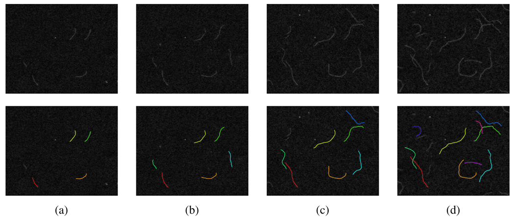
In Figure 3, we show tracking results of several frames during the entire tracking process of image sequence I.

Fig. 3.

Detecting and tracking filaments on image sequence I. (a) The 1st frame and computed snakes based on it, (b) the 6th frame and computed snakes based on it, (c) the 12th frame and computed snakes based on it, and (d) the 16th frame and computed snakes based on it.

30 filaments from the two image sequences were manually selected to measure tracking errors of our algorithm. For each frame, we manually labeled selected filaments’ two tip locations as ground truth and computed distances between them and the tips of automatically deformed snakes as tip tracking errors. We observed that filament bodies are segmented and tracked accurately by deformed snakes. The most errors resulting from tip tracking are due to filament intersections and low SNR at tip locations. When we observed a tracking failure, which means a snake stretched to two different filaments (see Figure 2(4)c), we reinitialized the snake in the next frame by hand and resumed tracking. Tracking error statistics are shown in Table 1.

Table 1.

Tip tracking error (distance between a labeled tip position and its corresponding snake tip) statistics of 30 filaments in image sequences I and II. (Unit: pixel)

Mean	Maximum	Standard Deviation	Number of Failures
1.4798	11.9332	1.7058	6 out of 810 (times)

Elongation rates of the two ends of each filament can be measured and calculated by finding a corresponding point between a snake in contiguous frames through registration (Section 2.3). Barbed and pointed ends were distinguished by their elongation rates because elongation rates of barbed ends are 10 times larger than that of pointed ends. The average elongation rates of barbed and pointed ends of above selected filaments in the image sequence I are shown in Table 2.

Table 2.

Measured average elongation rates of barbed and pointed ends of selected filaments in the image sequence I. The manual measurement were performed using the method of [7]. (Unit: mon/sec)

This Method		Manual Labeling [7]
Barbed End	Pointed End	Barbed End	Pointed End
11.2207	0.00621	11.2524	0.04634

4. CONCLUSION

In this paper, we proposed a new automated algorithm for actin filament segmentation and tracking. Open active contour models instead of closed ones are employed. A novel external energy term, which consists of an image term and a stretching term, helps snakes locate the center of filaments. Converged snakes at time t−1 are propagated to time t for initialization. Greater tip stiffness and “jump” strategies are proposed to solved filament intersection problem. Experimental and validation results demonstrated the performance of this method.

REFERENCES

- 1.Besl P, McKay H. A method for registration of 3-D shapes. TPAMI. 1992:239–256. [Google Scholar]
- 2.Fujiwara I, Takahashi S, Tadakuma H, Funatsu T, Ishiwata S. Microscopic analysis of polymerization dynamics with individual actin filaments. Nat. Cell Biol. 2002;4:666–673. doi: 10.1038/ncb841. [DOI] [PubMed] [Google Scholar]
- 3.Fujiwara I, Vavylonis D, Pollard TD. Polymerization kinetics of ADP- and ADP-Pi-actin determined by fluorescence microscopy. Proc. Natl. Acad. Sci. U. S. A. 2007;104:8827–8832. doi: 10.1073/pnas.0702510104. [DOI] [PMC free article] [PubMed] [Google Scholar]
- 4.Hadjidemetriou S, Toomre D, Duncan J. Motion tracking of the outer tips of microtubules. Medical Image Analysis. 2008;12:689–702. doi: 10.1016/j.media.2008.04.004. [DOI] [PubMed] [Google Scholar]
- 5.Kass M, Witkin A, Terzopoulos D. Snakes: Active contour models. IJCV. 1987;1:321–331. [Google Scholar]
- 6.Kong K, Marcus A, Giannakakou P, Wang M. Using particle filter to track and model microtubule dynamics. ICIP. 2007;5:517–520. [Google Scholar]
- 7.Kuhn JR, Pollard TD. Real-time measurements of actin filament polymerization by total internal reflection fluorescence microscopy. Biophys. J. 2005;88:1387–1402. doi: 10.1529/biophysj.104.047399. [DOI] [PMC free article] [PubMed] [Google Scholar]
- 8.Lindeberg T. Edge detection and ridge detection with automatic scale selection. IJCV. 1998;30:117–154. [Google Scholar]
- 9.Saban M, Altinok A, Peck A, Kenney C, Feinstein S, Wilson L, Rose K, Manjunath BS. Automated tracking and modeling of microtubule dynamics. ISBI. 2006:1032–1035. [Google Scholar]
- 10.Smal I, Draegestein K, Galjart N, Niessen W, Meijering E. Particle filtering for multiple object tracking in dynamic fluorescence microscopy images: Application to microtubule growth analysis. IEEE Trans. on Medical Imaging. 2008;27:789–804. doi: 10.1109/TMI.2008.916964. [DOI] [PubMed] [Google Scholar]