High Throughput Transmission Optical Projection Tomography Using Low Cost Graphics Processing Unit

Abstract

We implement the use of a graphics processing unit (GPU) in order to achieve real time data processing for high-throughput transmission optical projection tomography imaging. By implementing the GPU we have obtained a 300 fold performance enhancement in comparison to a CPU workstation implementation. This enables to obtain on-the-fly reconstructions enabling for high throughput imaging.

1. Introduction

Our understanding of gene function and system biology often relies on the ability to optically interrogate molecular and functional changes in intact organisms at high resolution. Unfortunately most optical imaging methods are not well suited for intermediate dimensions i.e. those that lie between the penetration limits of modern optical microscopy (0.5–1mm) and the diffusion-imposed limits of optical macroscopy (>1cm) [1]. Thus, many important model organisms, e.g. insects, animal embryos or small animal extremities, often remain inaccessible.

Several optical imaging techniques that have been recently introduced aim at filling this important gap. They do so by increasing the imaging penetration depth such as mesoscopic fluorescence tomography and selective plane photoacoustic tomography [2] [3]. Optical projection tomography is a recently developed three-dimensional imaging technique that is particularly well suited for developmental biology and gene expression studies of both absorptive and/or fluorescent samples. This technique has proven to be valuable for anatomical and histological applications. The technique is analogous to X-ray computed tomography as it works under the approximation of negligible light scattering. Samples are made transparent by substituting the cellular fluids with a solution that index matches the cell membranes and thereby eliminates the presence of any scattering component. Thus, the diffusive light contribution is almost null. This condition is first achieved by dehydrating the sample and by placing it for several hours in BABB or Murray’s Clear solution (a mixture of benzyl alcohol and benzyl benzoate in a 2:1 ratio). Once cleared, the samples present very low scattering and absorption values making their light diffusive contribution almost negligible. Fluorescence or absorption images (projections) of the samples are then taken over 360 degrees obtained with a fixed rotational angle along the vertical axis. The use of a lens with high telecentricity combined with a variable diaphragm, allows us to project on the CCD camera photons with light paths that are parallel to the optical axis [4].

3D tomographic reconstructions are widely used for medical and industrial imaging applications. Many different types of signal such as X-rays, gamma rays, electron-positron annihilation, white light and laser light can be exploited and processed to create a tomographic image. However, because these reconstructions represent a highly demanding computational problem, high throughput imaging capability is restricted. In order to achieve the necessary performance, both new reconstruction methods and hardware platforms must be implemented.

Reconstruction algorithms can be classified into two main categories: analytical and iterative. Since analytical methods are faster than the iterative ones, they are generally more suitable for real-time reconstructions with the algorithm choice depending on the information provided, such as the amount and the quality of the acquired projections.

While iterative reconstruction (IR) methods, such as the ones based on statistical reconstruction or algebraic reconstruction techniques, offer the advantage over the analytical ones to improve image contrast and resolution quality, they generally require a high number of iterations in order to achieve the same quality reconstruction compared to the analytical Filtered Back Projection algorithm. In fact, when projections are available from all directions and the signal-to-noise ratio (SNR) is high (noise is negligible), the filtered backprojection (FBP) reconstruction technique is the predominantly chosen method for most X-ray computed tomography. FBP is based on the mathematical problem, solved by Radon [5], of the determination of a function f from an infinite set of its line integrals. Due to the finite number of acquisitions that can be usually acquired, the reconstruction transform (inverse Radon transform formula) is modified into the discrete case [6]. To preserve the reconstructed image details, a high band pass filter is applied. The filtering operation can be implemented in the frequency or in the spatial domain. In the first case it is generally more computationally expensive than a convolution with a fixed impulse response.

Fast algorithms for reconstruction have been developed as well and are mostly based on the Fourier slice theorem [7–12], on mutilevel invertion of the Radon transform [13] or hierarchical decomposition of the backprojection operation [14]. Normally, the algorithm in parallel beam reconstruction is implemented as a triple nested “for” loop with O(N³) computational complexity, but fast algorithms are able to reduce it to O(N²log₂N). Unfortunately the use of fast algorithms for many real-time medical applications would be impossible without hardware acceleration.

Parallel processing is one of the available strategies which offers higher computing power with respect to CPU processing leading to considerable reduction in the processing time. Since tomographic reconstruction algorithms show a high level of data parallelism [15], many hardware implementations have been developed in the past few years in order to achieve real-time performance.

Focusing on hardware acceleration, there are two main strategies to improve image reconstruction speed. The first approach uses mainframe parallel computers such as PC clusters or specific devices such as Application Specific Integrated Circuits (ASICs) or Field Programmable Gate Arrays (FPGAs) connected to the memory through dedicated high-speed busses. Their complexity and cost make this option unappealing. The second solution uses a graphic processing unit (GPU). The GPU, which is based on a massively parallel computing architecture, is a high-performance device. Due to its processing power and low cost (currently around 1500 USD) is employed not only for graphics purposes but even for more general purpose computing (GPGPU), especially in the biomedical field where very large amounts of data have to be processed and expansive computations have to be performed, e.g. high-speed Monte Carlo simulation of photon migration or holographic microscopy [16].

Because of the efficiency of GPUs when dealing with repetitive data processing (often present in loops) they have been extensively employed in medical tomography [17], for example in cone beam computed tomography (CBCT) [18]. Filter Backprojection, which is the standard reconstruction algorithm for CBCT, in GPU implementation has proven to be hundreds of times faster when compared to CPU based implementation [19]. Moreover, the recent availability of NVIDIA’s common unified device architecture (CUDA) significantly reduces the complexity and the implementation of GPU programming.

Motivated by these appealing features we used a GPU to reduce the computational times for real time transmission OPT. To reconstruct 512³ and 1024³ volumes we chose to use a standard FBP Algorithm. We avoided iterative methods because of their computational complexity and because the SNR and the number of projections of OPT data sets were so high that non-IR algorithms were required. Our data show that a 300 fold enhancement of reconstruction speed can be achieved using a < 1500 USD GPU. Also note that there is a checklist available in Section 6 that summarizes the style specifications.

2. Experimental Section

The experimental setup is shown in Fig. 1. A white light source is filtered with two narrow band pass interference filters centered at the desired wavelength with a 5 nm full-width-at-half-maximum (FWHM). A set of filters allows for control of the amount of light directed onto the sample to fill the dynamic range of the CCD. Uniform sample illumination is critical and is achieved by using a beam expander with a combined two-lense Galilean telescope and a diffuser. The sample which is fixed in an agarose holder and immersed in a BABB solution is rotated along its vertical axis by a high speed rotational stage (Newport, PR50) with an absolute accuracy of 0.05 degrees. The sample vertical axis can be tilted and adjusted in its orthogonal plane by way of three distinct manual controllers.

Fig. 1.

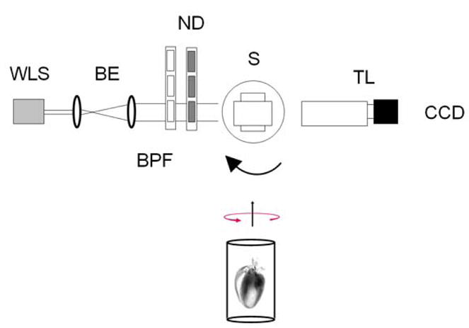
Experimental Setup. WLS white light source, BE beam expander, BPF band pass filters, ND optical density filters, S sample, TL telecentric lens imaging system.

The transillumination signal is directly detected by a CCD camera (Princeton Instruments, Trenton, NJ) with a 1024×1024 or a 512×512 (after 2×2 binning) imaging array using a telecentric system. Images are then taken over 360 projections with a 1 degree rotational angle along the vertical axis. The filters can be easily interchanged to perform multispectral imaging.

We studied a mouse heart which had previously sustained a controlled myocardial infarct (MI) induced by coronary ligation. The rodent model of coronary ligation is widely used in heart failure research and for instance led to the current treatment of post MI patients with ACE inhibitors. It can also be used to study wound healing dynamics and cardiac repair after ischemia.

Mouse were anesthetized with an intraperitoneally (IP) injection of a mix of ketamine (90 mg/kg) and xylazine (10mg/kg) followed by an IP injection of 50 U of heparin. Five minutes later, a longitudinal laparotomy was performed; the left renal vein was opened and 20ml of saline solution was infused into the IVC. After flushing out all the mouse blood, the heart was removed using a dissecting microscope and then fixed for 1 hour in 4% PFA solution at 4°C temperature and finally embedded in a 1% agarose gel. The sample was then dehydrated through a series of 20% to 100% ethanol solutions, and cleared by immersion in the BABB solution.

3. Backprojection Algorithm

Here we consider the problem of volumetric tomographic reconstruction of absorbed light from a scattering-free absorbing object illuminated by a collimated source and with projections acquired in transillumination mode. The reconstruction algorithm is based on the parallel beam filtered back-projection (FBP) method which is predominantly used for X-ray computed tomography.

The concept of projection and tomographic reconstruction can be mathematically introduced with the Radon transform (Fig. 2). Let f(x,y) be the image density distribution to be reconstructed. For OPT the image will correspond to the light absorption map of the sample under investigation. We then define the line integral of f along the line L at a distance s from the origin and at angle θ with the x-axis, as the Radon transform R̂f

Fig. 2.

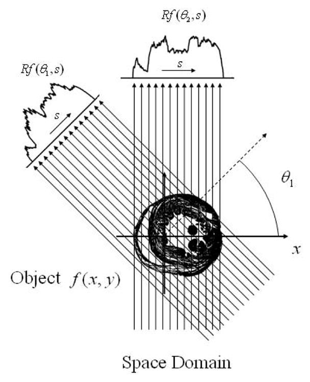
Schematic of the coordinate system used for parallel-beam backprojection. Parallel projections Rf(θ,s) in the space domain of an object f(x,y) at different angles.

$$\widehat{R}f(\theta ,s)=\int f(x,y)\delta (xcos\theta +ysin\theta )\mathit{dxdy}$$

With θ and s fixed, the integral R̂f(θ,s) is called projection which in parallel beam geometry, as is the case in first approximation for OPT due to the high telecentricity of the system and the lack of scattering present within the sample, consists of the sum of all parallel ray integrals. In OPT, the projections represent the optical transillumination CCD measurements. We can describe each ray emitted from an arbitrary source at position x_s in a discretized one-dimensional fashion (Fig. 3) as it passes through the absorbing object and before being collected by the CCD’s pixel located at position x_d as exponentially attenuated following a simple Beer-Lambert-type attenuation law given by

Fig. 3.

(a) Transillumination measurements. Parallel beams in the (x,y) plane are propagating from the source position x_s to the detector position x_d. (b) The attenuation along the direction of propagation for a beam with intensity I₀ follows a Beer-Lambert law.

$$I(x_s,x_d)=I_0{e}^{-{\mu }_{a}L}$$

Here I₀ represents the intensity of the source, x_s, L the thickness of the sample, and μ_a the absorption coefficient (if we consider μ_a a function of the two coordinates x,y this is equivalent to an image function f(x,y)=μ_a(x,y)).

The OPT or CT image reconstruction problem consists in computing f(x,y) given its Radon transform R̂f(θ,s), i.e. computing μ_a(x,y) given all the projections. The most commonly used algorithm for X-CT, and by extension to the OPT case, is the filtered backprojection method (FBP) which can be formulated as [20]:

$$f(x,y)=\underset{0}{\overset{\pi }{\int }}\underset{-\infty }{\overset{\infty }{\int }}{R}_{\theta }^{\ast }(\omega )\left|\omega \right|e^{i2\pi \omega (xcos\theta +ysin\theta )}d\omega d\theta$$

where R_θ^* is the Fourier transform of a profile R_θ taken at a fixed angle θ and where the multiplication by |ω| in the Fourier domain represents a filtering operation (ramp filter). The operation performed by the integral over the interval [0, π] calculates the back-projections. Note that for practical use the ramp filter is substituted with a function W_b(ω) = |ω|H (ω) where H is equal to 1 at low frequencies but approximates zero at the high ones [20]. Since the number of measured projections is finite, the integral will be replaced by sums over all the angles and the Fourier transform by the fast Fourier transform (FFT) over an even number of Fourier components.

4. Implementation

Reconstructions with the Radon backprojection algorithm were realized using the NVIDIA common unified device architecture (CUDA) technology [21]. This technology allows to perform a massive amount of similar calculations in parallel while distributing them on different multiprocessors. A CUDA-enabled Tesla C1060 was used to speed up calculations. This card consists of 240 streaming processors each running at 1.3 GHz with 4GB of dedicated GDDR3 onboard memory and ultrafast memory access with 102 GB/s bandwidth per GPU. The card is targeted as a high-performance computing (HPC) solution for PCI Express systems and is capable of 933 GFLOPs/s of processing performance.

For the programming of the GPU we utilize the CUDA technology that makes use of the unified shader design of the NVIDIA graphics processing unit [22–23]. With this architecture the GPU is handled as a coprocessor executing data-parallel kernel functions [24]. The NVIDIA compiler takes care of the CUDA instructions present in the user code.

NVIDIA tools were also utilized, such as “NVCC” NVIDIA compiler and “CUFFT” library for executing the Discrete Fourier Transform. C and C++ programming languages (MS VisualStudio 2005 Standard Edition) were used for software developing. The overall implementation is illustrated in Fig. 4

Fig. 4.

Scheme of the GPU implementation reconstruction algorithm.

For the reconstructions, we implemented two different ways of data processing. The first one is a post-processing strategy. All projection images are acquired, then all rows with number n from the different scans are moved into a separate matrix. Each row of this matrix is shifted to adjust for the real center of rotation and padded with zeros to filter the length. Because the process is symmetric for scans corresponding to K and (180-K) degrees of rotation angle, an optimization is applied: values from scans corresponding to an angle of rotation of (180-K) degree are reversed around the center of rotation and summarized with the values corresponding to a K degree scan. Note that such an optimization could be done only if we have corresponding pairs of scans. We then performed the calculations on each row of the matrix. First, we applied a 1D Discrete Fourier Transform, then the results are filtered using a Hamming filter for example, and finally a 1D Inverse Discrete Fourier Transform is applied. At the end the matrix is backprojected into the corresponding reconstruction slice number n (see Fig. 5). The required computations are mapped to the CUDA kernel executions with the procedure repeated for all the projection rows depending on the number of reconstructed slices needed.

Fig. 5.

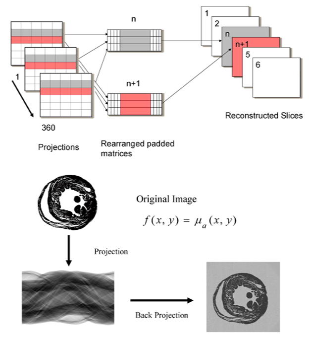
Backprojection reconstruction process.

Different arrays are first allocated in the Tesla memory, like the Hamming filter, the pre-calculated sinuses and cosines of rotation angles of the source scans, the X and Y coordinates of the reconstructed slices, and all the additional arrays necessary for the calculations (e.g. for the complex Fourier Transform or for the resulting set). These operations are therefore performed only once. Then a rearranged (shifted, padded and summarized) matrix is copied to the Tesla memory and all the above steps – conversion of the matrix to complex format, complex FFT, filtering, complex IFFT, backprojection - are performed by the Tesla on-board as kernels, i.e. in parallel. (See Fig. 6)

Fig. 6.

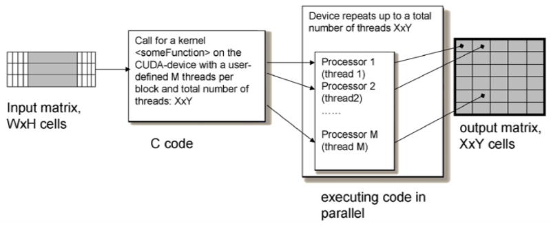
Scheme of the kernel executed on the CUDA-device.

The FFT and IFFT from the “CUFFT” library of the CUDA package were used in a batch mode. Texturing was applied in the kernel functions, considerably speeding up the calculations. The resulting reconstructed slices were copied back to host. All the manually defined parameters for the CUDA-device such as block size and batch size depend on the projection image size and available device memory and are therefore experimental and platform dependent.

The second reconstruction strategy we implemented consists of processing all the scans one by one as they appear in the file system of the host. This modality requires much more Tesla card memory as well as host memory. The difference to the previous method is that all the reconstructed slices are kept in the Tesla memory. This allows for summarization of the previous values of the reconstructed set with the result for the currently handled scans. This is possible for small sets only (e.g. 512×512×512). For 1024×1024×1024 the reconstructed set itself takes 4GB of memory for float values therefore additional copying operations are required to put appropriative part of the reconstructed set for the current scan into the card memory. Also, for one-by-one processing we cannot optimize with K and (180-K) degree scans summarizing. This processing strategy is particularly useful for producing on-the-fly reconstructions.

In addition, we tested a direct convolution operation with short-length filters. The resultant time for convolution on Tesla was rather close to <FFT - Hamming filter – IFFT> way of calculating, especially for large sets.

4. Results

All reconstructions were performed on a Intel Core at 3.16 GHz with 3 GB of main memory equipped with the Nvidia Tesla C1060 and running Windows XP.

For the following experiments we used 360 projections of size 512² or 1024² each to reconstruct a 512³ or 1024³ volume. Saggital, longitudinal, axial, and 3D reconstructions of the heart data utilized in this work are shown in Fig. 7.

Fig. 7.

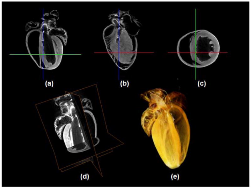
Reconstructed image results for the absorption coefficient for 360 projections. Selected sections of the reconstructed images at three different planes (saggital (a), longitudinal (b), axial (c)) as shown in (d). (e) 3D rendering (Media 1).

Table 1 and 2 compare the performances for both CPU- and GPU-based configurations when using the two different implementations mentioned above. In both tables, we present the timing for the overall reconstructions. We also give the numbers of the back-projected projections and the numbers of volume slices.

Table 1.

Comparison of reconstruction times between GPU and CPU.

Image Size (512×512×512)
Time (sec) GPU	Time (sec) CPU	Accel. (fold)	Read	Write	Algorithm
3.8	1228	323	No	No	FFT
14.6	2048	140	Yes	Yes	FFT
14.5	1280	89	No	Yes	FFT
4.3	1250	291	No	No	Convolution (21 values)
Image Size (1024×1024×1024)
Time (sec) GPU	Time (sec) CPU	Speed up	Read	Write	Algorithm
36	9932	276	No	No	FFT
65	14848	228	Yes	Yes	FFT
62	10500	170	No	Yes	FFT
31	9932	321	No	No	Convolution (21 values)

Table 2.

Comparison of reconstruction times between GPU and CPU (on-the-fly reconstructions).

Image Size (512×512×512)
Time (sec) GPU	Read	Write	Algorithm
14.5	Yes	No	FFT
14.6	Yes	Yes	FFT
Image Size (1024×1024×1024)
Time (sec) GPU	Read	Write	Algorithm
207	No	No	FFT
281	Yes	Yes	FFT*

^*results copied to host in 4 readings

The GPU card significantly accelerates the reconstruction speed. Our results indicate an effective 300-fold acceleration compared to a standard single-threaded CPU based implementation. For 512³ volumes typical times were around 3.8 s, while for 1024³ volumes times of the order of 36 sec were obtained.

The overall reconstruction time can be further reduced by considering fewer projections. This option can be used when the single projection exposure time has to be kept very long e.g. while acquiring fluorescence signal where typical times in the order of 10’s of seconds could be required, but we want to keep the overall acquisition time very short, as is the case for fast screening. Obviously, the quality of the reconstructions is quite reduced at the expense of the speed. In Fig. 8, different reconstructions are shown for projections taken with an angle step of 10,5,3, and 1 degrees, respectively.

Fig. 8.

Sagittal (a), longitudinal (b), and axial (c) reconstructions obtained with projections taken every 10,5,3, and 1 degrees.

In Table 2, we present the timing for on-the-fly reconstructions obtained with 360 projections. On-the-fly reconstructions are very useful to provide a direct feedback during an OPT acquisition, while postprocessing of the data is mostly required, in particular, for fine tuning the position of the center of rotation or correction of the rotational axis’ tilting angle or the imaging optics. In this case, data are processed while being simultaneously acquired, providing real time feedback on the reconstructions. The acquisition and visualization program is made in Labview and is resident on a separate PC from the one hosting the GPU. Data between the two PCs are exchanged via Ethernet cable. The times indicated in the table are obtained for single projections virtually acquired with acquisition time equal to zero in order to give a minimum time limit. Because acquisition times are dependent on the exposure time and the sample rotational speed, processing times could be considerably longer. In our setup on-the-fly transmission OPT reconstruction times are limited mostly by the speed of our rotational stage (4 minutes with 100 msec acquisition time).

Intermediate transmission OPT reconstructions at 45, 90, 180, and 360 degrees obtained on-the-fly are shown in Fig. 9. These images were produced in real time while imaging the sample. Due to the non-perfect telecentricity of the system, projections over 360 degrees need to be taken. Reconstructions acquired over 180 (a) and 360 (b) degrees are shown in Fig. 10. The corresponding zoomed areas (c and d respectively) clearly show the improvement in the resolution and the need for acquiring over 360 degrees. A histological section of the imaged heart at approximately the same height is shown in comparison in (e), indicating a good correlation between reconstructions and histology.

Fig. 9.

On-the-fly sagittal (a) and axial (b) reconstructions with projections taken every one degree. The projections are displayed in real time during acquisition.

Fig. 10.

Axial reconstructions obtained after the acquisition of 180 (a) or 360 (b) projections. (c) and (d) correspondent zoomed area. Histological section at approximately the same height (e).

Conclusion

In conclusion, we presented a CUDA-enabled GPU system for real time transmission Optical Projection Tomography. With relatively modest cost, the system provides a massive, 300-fold acceleration compared to traditional CPU based systems and thus offers high throughput OPT and real time data processing. Due to the current low prices of GPUs, our solution is particularly attractive. The capability to obtain on-the-fly reconstruction visualizations is very useful for correcting problems during acquisition. Future directions will aim at using the same technology in order to obtain fluorescence tomographic reconstructions, a case for which the standard backprojection algorithm produces erroneous signal distribution and where instead a Born normalized approach that accounts for tissue absorption needs to be implemented.