An Automatic 3D Mesh Generation Method for Domains with Multiple Materials

Abstract

This paper describes an automatic and efficient approach to construct unstructured tetrahedral and hexahedral meshes for a composite domain made up of heterogeneous materials. The boundaries of these material regions form non-manifold surfaces. In earlier papers, we developed an octree-based isocontouring method to construct unstructured 3D meshes for a single-material (homogeneous) domain with manifold boundary. In this paper, we introduce the notion of a material change edge and use it to identify the interface between two or several different materials. A novel method to calculate the minimizer point for a cell shared by more than two materials is provided, which forms a non-manifold node on the boundary. We then mesh all the material regions simultaneously and automatically while conforming to their boundaries directly from volumetric data. Both material change edges and interior edges are analyzed to construct tetrahedral meshes, and interior grid points are analyzed for proper hexahedral mesh construction. Finally, edge-contraction and smoothing methods are used to improve the quality of tetrahedral meshes, and a combination of pillowing, geometric flow and optimization techniques is used for hexahedral mesh quality improvement. The shrink set of pillowing schemes is defined automatically as the boundary of each material region. Several application results of our multi-material mesh generation method are also provided.

1 Introduction

With finite element analysis seeing increased use in active research areas such as computational medicine and computational biology, there is an emerging need for quality mesh generation of the spatially realistic domains that are being studied. In Computer Tomography (CT) imaging as in Magnetic Resonance Imaging (MRI) of the human body, the domain of focus often possesses heterogeneous materials and/or functionally different properties. For example, as shown in Figure 1, the MRI brain data has been segmented into 48 sub-areas, with each colored area demarked as possessing specific characteristic functionality. In finite element analysis, heterogeneous materials are grouped into separate material regions with individual physical/chemical attributes or material coefficients. For this purpose, quality meshes are needed for each of the partitioned material regions, with meshes conforming at the material boundaries. Such multi-material domain meshing is the focus of this paper.

Fig. 1.

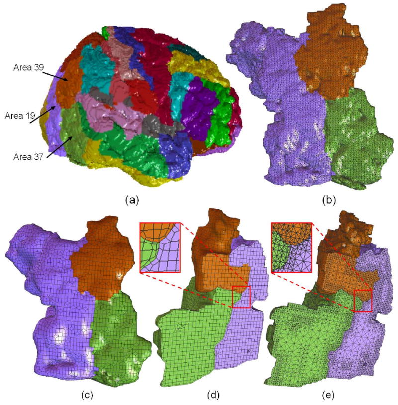
Mesh generation for the segmented Brodmann brain atlas with 48 areas or materials. In (b)-(e), only three areas (Areas 19, 37, and 39) are shown. (a) - smooth shading of the constructed brain model, each color represents one material; (b) - a triangular mesh; (c) - a quadrilateral mesh; (d) - one cross-section of a hexahedral mesh; (e) - one cross-section of a tetrahedral mesh. Red windows show details.

In [33, 32], we developed an octree-based isocontouring method to construct adaptive and quality tetrahedral/hexahedral meshes from imaging data with meshes conforming to boundaries defined as level sets. However these prior methods work only for a domain with a single material and manifold boundary. In order to automatically construct 3D meshes for all the material regions at the same time, we introduce and analyze a so-called material change edge to relocate all non-manifold boundaries, including the boundaries of each material domain and the interfaces between two or more materials. A novel approach is developed to calculate non-manfold boundary nodes within boundary cells shared by more than two materials. All the surface boundaries are meshed into triangles or quadrilaterals. Besides the material change edge, we also analyze each interior edge for each material domain to construct tetrahedral meshes. Each interior grid point is analyzed for hexahedral mesh construction.

Mesh adaptivity can be controlled in different ways: by a feature sensitive error function, by regions that users are interested in, by finite element solutions, or by a user-defined error function. The feature sensitive error function measures topology and geometry changes between isocontours at two neighboring octree levels. Adaptive tetrahedral and hexahedral meshes are generated by balancing the above four criteria and mesh size. Edge contraction and geometric flows [34] are used to improve the quality of tetrahedral meshes. A combination of pillowing, geometric flow, and optimization techniques is chosen for quality improvement of hexahedral meshes. With shrink set defined in an automatic way, the pillowing technique guarantees for each element in hexahedral meshes that at most one face lies on the boundary. This provides us with considerable freedom to further improve the element aspect ratio, especially for elements along the boundary.

We have applied our meshing method on a segmented human brain and rice dwarf virus (RDV) data, both containing multiple materials. Quality tetrahedral and hexahedral meshes are generated automatically with conforming boundaries, and some quantitative statistics such as area and volume for each domain are computed. Our results provide useful information to check the anatomy of the human brain, or to identify and understand the RDV structure.

The remainder of this paper is organized as follows: Section 2 summarizes related prior work. Section 3 reviews the octree-based unstructured mesh generation techniques we had developed. Section 4 discusses the detailed algorithm of mesh generation for a domain with multiple materials. Section 5 explains how to improve the mesh quality using various techniques. Section 6 presents some of our quality meshing results. Section 7 draws conclusions and outlines future work.

2 Previous Work

Octree-based Mesh Generation

The octree technique [30, 24], primarily developed in the 1980s, recursively subdivides the cubes containing the geometric model until the desired resolution is reached. Irregular cells are formed along the geometry boundary, and tetrahedra are generated from both the irregular cells on the boundary and the interior regular cells. Unlike Delaunay triangulation and advancing front techniques, the octree technique does not preserve a pre-defined surface mesh. The resulting meshes also change as the orientation of octree cells changes. In order to generate high quality meshes, the maximum octree level difference during recursive subdivision is restricted to be one. Bad elements may be generated along the boundary, therefore quality improvement is necessary after mesh generation.

The grid-based approach generates a fitted 3D grid of structured hexahedral elements on the interior of the volume [22]. In addition to regular interior elements, hexahedral elements are added at the boundaries to fill gaps. The grid-based method is robust, however it tends to generate poor quality elements along the boundary. The resulting meshes are also highly dependent upon the grid orientation, and all elements have similar sizes. A template-based method was developed to refine quadrilateral/hexahedral meshes locally [23].

Quality Improvement

Algorithms for mesh improvement can be classified into three categories [27] [20]: local refinement/coarsening by inserting/deleting points, local remeshing by face/edge swapping, and mesh smoothing by relocating vertices. Laplacian smoothing generally relocates the vertex position at the average of the nodes connecting to it. Instead of relocating vertices based on a heuristic algorithm, an optimization technique to improve the mesh quality can be utilized. The optimization algorithm measures the quality of the surrounding elements to a node and attempts to optimize it. The optimization-based smoothing yields better results, but is more expensive. Therefore, a combined Laplacian/optimization-based approach was recommended [6, 8], which uses Laplacian smoothing whenever possible and only uses optimization-based smoothing when necessary. Furthermore, related mesh quality improvement techniques use a combination of quadrilateral/hexahedral subdivision, anisotropic remeshing, and those based on conformal remapping [3, 4, 1, 2, 7].

Pillowing Techniques

A “Doublet” is formed when two neighboring hexahedra share two faces, which have an angle of at least 180 degrees. In this situation, it is practically impossible to generate a reasonable Jacobian value by relocating vertices. The pillowing technique was developed to remove doublets by refining quadrilateral/hexahedral meshes [17, 5, 26, 25]. Pillowing is a sheet insertion operation, which provides a fairly straightforward method to insert sheets into existing meshes. The speed of the pillowing technique is largely dependent upon the time needed to determine the shrink set. The number of newly introduced hexahedra equals the number of quadrilaterals on the inserted sheet.

We have developed octree-based isocontouring methods to construct tetrahedral and hexahedral meshes from gridded imaging data [33, 32]. In this paper, we extend these methods to automatic tetrahedral/hexahedral mesh generation for a domain with multiple materials. In addition, we will also discuss how to automatically define the shrink set and use the pillowing technique to improve the quality of hexahedral meshes.

3 A Review of the Octree-based Isocontouring Method for Mesh Generation

There are two main isocontouring methods, primal contouring (or Marching Cubes) and Dual Contouring. The Marching Cubes algorithm (MC) [16] visits each cell in a volume and performs local triangulation based on the sign configuration of the eight vertices. MC and its variants have three main drawbacks: (1) the resulting mesh is uniform, (2) poor quality elements are generated, and (3) sharp features are not preserved. By using both the position and the normal vectors at each intersection point, the Dual Contouring method [12] generates adaptive isosurfaces with good aspect ratio and preserves sharp features. In this section, we are going to review the Dual Contouring method, and the octree-based algorithms we developed for 3D mesh generation.

3.1 Dual Contouring Method

The octree-based Dual Contouring method [12] analyzes each sign change edge, which is defined as one edge whose two end points lie on different sides of the isocontour. For each octree cell, if it is passed by the isocontour, then a minimizer point is calculated within this cell by minimizing a predefined Quadratic Error Function (QEF) [9, 10],

$$\mathit{QEF}(x)=\sum _i{\left(n_i\cdot \left(x-p_i\right)\right)}^2$$ (1)

where p_i and n_i represent the position and unit normal vectors of the intersection point, respectively. For example, in Figure 2, the red curve is the true curve inside an octree cell, and the two green points are intersection points of the red curve with cell edges. The calculated minimizer point (the red one) is actually the intersection point of the two tangent lines.

Fig. 2.

A minimizer point (the red one) is calculated within an octree cell as the intersection point of two tangent lines. The two green points are intersection points of the red curve with cell edges. p_i and n_i are the position and unit normal vector at a green point, respectively.

In the uniform case, each sign change edge is shared by four cells, and one minimizer point is calculated for each of them to construct a quadrilateral. In the adaptive case, each sign change edge is shared by either four cells or three cells, and we obtain a hybrid mesh, including quadrilateral and triangular elements.

3.2 Tetrahedral Mesh Generation

We have extended the Dual Contouring method to tetrahedral mesh generation [33, 36]. Each sign change edge belongs to a boundary cell, which is an octree cell passed through by the isocontour. Interior cells only contain interior edges. In order to tetrahedralize boundary cells, we analyze not only sign change edges but also interior edges. Only interior edges need to be analyzed for interior cell tetrahedralization. Each sign change edge is shared by four or three cells, and we obtain four or three minimizer points. Therefore these minimizers and the interior end point of this sign change edge construct a pyramid or tetrahedron. For each interior edge, we can also obtain four or three minimizers. Those minimizers and the two end points of this interior edge construct a diamond or pyramid. A diamond or pyramid can be split into four or two tetrahedra. Finally, the edge contraction and smoothing method is used to improve the quality of the resulting meshes.

3.3 Hexahedral Mesh Generation

Instead of analyzing edges, we analyze each interior grid point to construct hexahedral meshes from volumetric data [32]. In a uniform case, each grid point is shared by eight octree cells and we can obtain eight minimizers to construct a hexahedron. There are three steps to construct adaptive hexahedral meshes: (1) a starting octree level is selected to construct a uniform hexahedral mesh, (2) templates are used to refine the uniform mesh adaptively without introducing any hanging nodes, (3) an optimization method is used to improve the mesh quality.

The octree-based meshing algorithms [33, 36, 32] we developed are very robust, and they work for complicated geometry and topology. However, they work only for a domain with a single material. In the following section, we will discuss how to construct 3D meshes for a domain with multiple materials.

4 Mesh Generation for A Domain with Multiple Materials

4.1 Problem Description

Given a geometric domain Ω consisting of N closed material regions, denoted as Ω₀, Ω₁, …, and Ω_N−1, it is obvious that ${\cup }_{i=1}^{N-1}$ Ω_i is the complement of Ω₀ in Ω moduls the boundary of Ω₀. Suppose B_i is the boundary of Ω_i, we have Ω_i ∩ Ω_j = B_i ∩ B_j when i ≠ j. ∪B_i may not always be manifold, it can also be non-manifold curves or surfaces. Figure 3 shows two examples in 2D. There are three materials in Figure 3(a) denoted as Ω₀, Ω₁ and Ω₂, and we can observe that ∪B_i are manifold curves. In Figure 3(b), there are four materials, but ∪B_i consists of non-manifold curves and a square outer boundary. Non-manifold boundaries ∪B_i cannot be represented by isocontours because each data point in a scalar domain can only have one function value. Therefore isocontouring methods do not work for a domain with non-manifold boundaries.

Fig. 3.

A domain with multiple materials. (a) - (∪)B_i consists of manifold curves; (b) - (∪)B_i consists of non-manifold curves and a square outer boundary.

One possible way to mesh a domain with non-manifold boundaries is to consider only one material region at a time using the method of function modification and isocontouring [33, 36, 32]. After meshes for all material regions are obtained, we merge them together. However, there are four problems in this method:

1. During the whole process, we have to choose the same octree data structure, including interfaces between two different materials. Otherwise the resulting meshes are not conforming to the same boundary.

2. When we mesh each material domain, we detect all boundaries surrounding this material. Part of the boundaries may be shared by more than two materials, for example, the red point in Figure 3(b) is shared by four materials, Ω₀, Ω₁, Ω₂, and Ω₃. When we process each material, we may obtain four different points to approximate the red one. In other words, the meshes obtained may not conform to each other around the interface shared by more than two materials.

3. It is difficult to find the corresponding points on the interface shared by two materials if only position vectors are given.

4. Since we analyze only one material region at a time, we need to process the data N times for a domain with N materials. This is very time consuming.

In this section, we are going to present an approach to automatically detect all boundaries and mesh a domain with multiple materials simultaneously. Here are some definitions used in the following algorithm description:

Boundary Cell

A boundary cell is a cell which is passed through by the boundary of a material region.

Interior Cell

An interior cell is a cell which is not passed through by the boundary of any material region.

Material Change Edge

A material change edge is an edge whose two end points lie in two different material regions. A material change edge must be an edge in a boundary cell.

Interior Edge

An interior edge is an edge whose two end points lie inside the same material region. An interior edge is an edge in a boundary cell, or an interior cell.

Interior Grid Point

An interior grid point of one material is a grid point lying inside this material region.

4.2 Non-Manifold Boundary Node Calculation

In our octree-based method, only one minimizer point is calculated for each cell, and each octree cell has a unique index. This property provides us a lot of convenience to uniquely index the minimizer point of octree cells without introducing any duplicates. Regarding meshing a domain with multiple materials which forms non-manifold boundaries, the challenging problem is how to calculate non-manifold boundary node within a cell shared by more than two materials.

There are two kinds of octree cells in the analysis domain: interior cells and boundary cells. For each interior cell, we simply choose the center of the cell as the minimizer point. For each boundary cell, we cannot separately calculate the minimizer point using Equation (1) for each material region because different minimizers may be obtained within this cell. For example in Figure 4(a), the red curve is the boundary which is shared by two materials Ω₁ and Ω₂. The same minimizer (the red point) is obtained when we mesh each material separately. However in Figure 4(b), there are three materials inside the octree cell, Ω₁, Ω₂ and Ω₃, and the blue point is shared by all three materials. Three different minimizers (the red points) are obtained for this cell when we mesh each material separately. Therefore instead of meshing each material separately, we include all intersection points (green points) in the quadratic error function (QEF) and calculate one identical minimizer point within this cell no matter how many materials are contained in it, which forms a non-manifold boundary node in the resulting mesh and guarantees conforming meshes around boundaries.

Fig. 4.

Minimizer point calculation within a boundary octree cell. The red curves are boundaries between materials, green points are intersection points of red curves with cell edges, and red points are calculated minimizers. (a) - the boundary is shared by two materials, and the same minimizer is obtained when we mesh each material separately; (b) - the octree cell contains three materials, and the blue point is shared by all the three materials. Three different minimizers are obtained within this cell when we mesh each material separately.

Our meshing algorithm assumes that only one minimizer is generated in a cell. When complicated topology appears in the finest cell, non-manifold surface may be constructed. Schaefer et al. extended the dual contouring method to manifold surface generation [21], but multiple minimizers were introduced within a cell. This cannot be further extended to 3D hexahedral mesh generation. Here we prefer a heuristic subdivision method. If a cell contains two components of the same material boundary, we recursively subdivide the cell into eight identical sub-cells until each sub-cell contains at most one component of the same material boundary. The subdivision method can be easily extended to hexhedral mesh generation, but it may introduce many elements. Fortunately, complicated topology rarely happens in a cell, for example in the segmented brain data (Figure 1) and the RDV data (Figure 14), this situation does not exist.

Fig. 14.

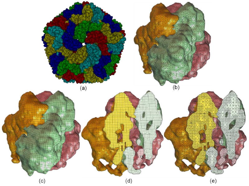
Mesh generation for the segmented rice dwarf virus (RDV) data. (a) - smooth shading of the segmented RDV model [31], each color represents four 1/3 trimers; (b) - a triangular mesh of one trimer consisting of three monomers; (c) - a quadrilateral mesh of one trimer; (d) - one cross-section of a hexahedral mesh; (e) - one cross-section of a tetrahedral mesh.

4.3 2D Meshing

4.3.1 2D Triangulation

Material change edges and interior edges are analyzed to construct triangular meshes for each material region as shown in Figure 5:

1. Material change edge: each material change edge is shared by two boundary octree cells in a uniform case, and one minimizer point is calculated by minimizing the quadratic error function defined in Equation (1). We can obtain two minimizer points. The two minimizer points and each end point of the material change edge construct a triangle. Therefore two triangles are obtained. In an adaptive case, each material change edge is also shared by two boundary octree cells, but the two octree cells may have different sizes. We can also get two minimizer points and construct two triangles.

2. Interior edge: each interior edge is shared by two octree cells. If the octree cell is a boundary cell, then we use Equation (1) to calculate a minimizer point. Otherwise we choose the center of this cell to represent the minimizer point. This interior edge and one minimizer point construct a triangle, therefore two triangles are obtained. In a uniform case, the two octree cells have the same size, while in an adaptive case, the two octree cells may have different sizes. However, we use the same method to construct triangles.

Fig. 5.

2D triangulation for a domain with multiple materials. (a) - there are three materials, and (∪)B_i constructs manifold curves; (b) - there are four materials, and (∪)B_i constructs non-manifold curves and a square outer boundary.

4.3.2 2D Quadrilateral Meshing

Instead of analyzing edges such as material change edges and interior edges, we analyze each interior grid point to construct a quadrilateral mesh. In a uniform case, as each interior grid point is shared by four octree cells, we can calculate four minimizer points to construct a quadrilateral. Six templates defined in [32] are used to refine the mesh locally. As shown in Figure 6(a, b), some part of the domain is refined using templates. The mesh quality improvement will be discussed later.

Fig. 6.

2D quadrilateral meshing for a domain with multiple materials. (a) - there are three materials, and (∪)B_i constructs manifold curves; (b) - there are four materials, and (∪)B_i constructs non-manifold curves and a manifold outer boundary.

4.4 3D Meshing

4.4.1 Tetrahedral Meshing

We analyze each edge in the analysis domain, which contains multiple material regions. The edge can be a material change edge or an interior edge. In a 3D uniform case, each edge is shared by four cells. We obtain a total of four minimizers, which construct a quadrilateral. The quadrilateral and the two end points of the edge construct two pyramids as shown in Figure 7(a), and each pyramid can be divided into two tetrahedra. In the 3D adaptive case, each edge is shared by four or three octree cells. Therefore we can obtain four or three minimizers, which construct a quadrilateral or a triangle. The quadrilateral/triangle and the two end points of the edge construct a diamond or a pyramid as shown in Figure 7(a, b). Finally we split it into tetrahedra.

Fig. 7.

Material change edges and interior edges are analyzed in 3D tetrahedralization. (a) - the red edge is shared by four cells, and two pyramids are constructed; (b) - the red edge is shared by three cells, and two tetrahedra are constructed. The green points are minimizer points.

We have applied our approach to an example with three materials. In Figure 8, a wireframe of the domain is shown in (a), (b) shows the constructed triangular mesh for the surface, and (c) shows one cross-section of the tetrahedral mesh for all three material regions. Note the presence of conforming boundaries.

Fig. 8.

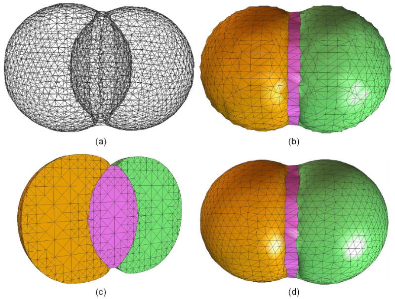
Tetrahedral mesh generation for a domain with three materials. (a) - a wireframe visualization; (b) -the constructed triangular surface mesh; (c) - one cross-section of the constructed tetrahedral mesh; (d) - the surface mesh is improved by using edge-contraction and geometric flow (100 steps with step length 0.01).

4.4.2 Hexahedral Meshing

For hexahedral mesh generation, we first choose a starting octree level and analyze each interior grid point in the uniform case. In 3D, each grid point is shared by eight octree cells, so we can obtain eight minimizer points to construct a hexahedron. An error function is calculated for each octree cell and is compared with a pre-defined threshold to decide the configuration of the minimizer point for this cell. All configurations can be converted into five basic cases defined in [32, 23], which are used as templates to refine the uniform mesh adaptively without introducing any hanging nodes. The templates satisfy one criterion: in all templates, the refinement around any minimizer points/edges/faces with the same configuration is the same. This criterion guarantees that no hanging nodes are introduced during the process of mesh refinement. Figure 9(a) shows quadrilateral meshes constructed for a domain with three materials. Figure 9(c) shows one cross-section of the hexahedral mesh.

Fig. 9.

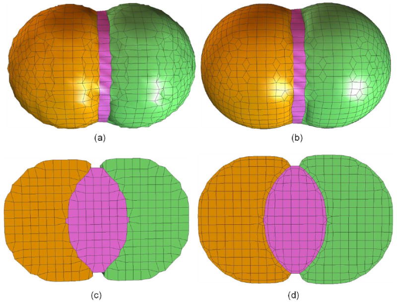
Hexahedral mesh construction for a domain with three materials. (a) - surface quadrilateral mesh; (b) - surface mesh after quality improvement with geometric flow (100 steps with step length 0.01); (c) - one cross-section of the original hexahedral mesh; (d) - one cross-section of the improved hexahedral mesh.

4.5 Mesh Adaptivity

The mesh adaptivity is controlled flexibly by different techniques:

1. A feature sensitive function defined in [33] is based on a trilinear function fⁱ(x, y, z) within an octree cell,

   $$F=\sum \frac{\left|f^{i+1}-f^i\right|}{\left|\nabla f^i\right|}$$ (2)

   where

   $$\begin{array}{l}{f}^i(x,y,z)=f_{000}(1-x)(1-y)(1-z)+f_{001}(1-x)(1-y)z\hfill \\ +f_{010}(1-x)y(1-z)+f_{100}x(1-y)(1-z)\hfill \\ +f_{011}(1-x)yz+f_{101}x(1-y)z\hfill \\ +f_{110}xy(1-z)+f_{111}\mathrm{xyz}.\hfill \end{array}$$ (3)

   f_lmn (where l, m, n = 0 or 1) is the function value at a grid point of the octree cell. The feature sensitive error function measures the isocontour difference between two neighboring octree levels, Level i and Level (i + 1).

2. Regions that users are interested in: According to various application requirements, location can be included in the error function to control the mesh adaptivity.

3. Finite element solutions: Finite element solutions can be used to efficiently and dynamically control the mesh adaptivity.

4. User-defined error function: Our algorithm is very flexible, and a user-defined error function can be substituted into the code for the mesh adaptivity control.

5 Quality Improvement

Mesh quality is a very important factor influencing the convergence and stability of finite element solvers. In the meshes generated from the above algorithm, most elements have good aspect ratio, especially the interior elements, but some elements around the boundaries may have poor aspect ratio, therefore the mesh quality needs to be improved.

5.1 Tetrahedral Mesh

First we choose three quality metrics to measure the quality of tetrahedral meshes, then use edge-contraction and geometric flow smoothing to improve it. The three quality measures are: (1) edge-ratio, which is defined as the ratio of the longest edge length to the shortest edge length in a tetrahedron; (2) Joe-Liu parameter $\frac{2^{\frac{4}{3}}\times 3\times {\left|V\right|}^{\frac{2}{3}}}{{\sum }_{0\le i<j\le 3}{\left|e_{ij}\right|}^2}$, where |V| denotes the volume, and e_{i j} denotes the edge vectors representing the 6 edges [15]; (3) Minimum volume bound.

Edge-contraction

We detect the element with the worst edge-ratio, and use the edge-contract method to remove it until the worst edge-ratio arrives at a predefined threshold, e.g., 8.5. A special case is shown in Figure 10. When one vertex P is embedded in a triangle T_tri or a tetrahedron T_tet, this vertex and each edge of T_tri construct a triangle in 2D, or this vertex and each face of T_tet construct a tetrahedron in 3D. If we contract any edge of T_tri or T_tet before removing the vertex P, then we will generate two duplicated and useless elements. This special case needs to be detected, and duplicated vertices/elements and useless vertices need to be removed after edge-contraction.

Fig. 10.

A special case for edge-contraction. In (a), a point P is embedded in a triangle P₀P₁P₂. P and each edge of the triangle P₀P₁P₂ construct a triangle. In (b), a point P is embedded in a tetrahedron P₀P₁P₂P₃. P and each face of the tetrahedron P₀P₁P₂P₃ construct a tetrahedron. When we contract any edge of triangle P₀P₁P₂ or tetrahedron P₀P₁P₂P₃, duplicated and useless elements are generated.

Geometric flow smoothing

There are two kinds of vertices in 3D meshes, boundary vertices and interior vertices. For each boundary vertex, we use geometric flow to denoise the surface and improve the aspect ratio. For each interior vertex, we use the weighted averaging method to improve the aspect ratio, e.g., volume-weighted averaging. During the smoothing process, the Joe-Liu parameter and minimum volume bound are chosen as the quality metrics.

Geometric flow or geometric partial differential equations (PDEs) have been intensively used in surface and image processing [28, 29]. Here we choose surface diffusion flow to smooth the surface mesh because it preserves volume. A discretization scheme for the Laplace-Beltrami operator over triangular meshes is given in [29] and so we do not go to detail here.

The main aim of edge-contraction is to improve the element with the worst edge-ratio for each iteration. However, the edge-contraction method cannot remove slivers, therefore we should couple it with the smoothing scheme. Geometric flow smoothing tends to improve the mesh globally. We repeat running the two steps until a threshold or an optimized state is reached.

Figure 8 shows the difference of the mesh before and after the quality improvement. Figure 8(b) shows the original mesh, and Figure 8(d) shows the improved mesh. It is obvious that after quality improvement, the surface mesh is more regular and has better aspect ratio. Figure 13 shows some statistics of quality metrics for the Brodmann brain atlas (Figure 1) and the segmented RDV data (Figure 14). The worst Joe-Liu parameter of the resulting meshes is above 10⁻².

Fig. 13.

The histogram of Joe-Liu parameter (left) of tet meshes, and the condition number (right) of hexahedral meshes for the human brain and the RDV data. It is obvious that the mesh quality, especially the worst parameter, is improved

5.2 Hexahedral Mesh

Knupp et al. defined the Jacobian matrix of a vertex using its three edge vectors [13, 14], here we choose the usual definition of the Jacobian matrix in the Finite Element Method [19, 11]. Given a hexahedron with eight vertices as shown in Figure 11, there is a basis function φ_i in terms of ξ, η and ζ corresponding to each of them in the parametric domain. The eight basis functions are:

Fig. 11.

A hexahedron [p1p2…p8] is mapped into a trilinear parametric volume in terms of ξ, η, and ζ. The eight basis functions in Equation (4) correspond to the eight vertices of the hexahedron.

$$\begin{array}{l}{\varphi }_1=(1-\xi )(1-\mathrm{\eta })(1-\mathrm{\zeta }),\hfill \\ {\varphi }_2=\mathrm{\xi }(1-\mathrm{\eta })(1-\mathrm{\zeta }),\hfill \\ {\varphi }_3=(1-\mathrm{\xi })\mathrm{\eta }(1-\mathrm{\zeta }),\hfill \\ {\varphi }_4=\mathrm{\xi }\mathrm{\eta }(1-\mathrm{\zeta }),\hfill \\ {\varphi }_5=(1-\mathrm{\xi })(1-\mathrm{\eta })\mathrm{\zeta },\hfill \\ {\varphi }_6=\mathrm{\xi }(1-\mathrm{\eta })\mathrm{\zeta },\hfill \\ {\varphi }_7=(1-\mathrm{\xi })\mathrm{\eta }\mathrm{\zeta },\hfill \\ {\varphi }_8=\mathrm{\xi }\mathrm{\eta }\mathrm{\zeta }.\hfill \end{array}$$ (4)

For any point inside this parametric hexahedral element, its coordinates can be calculated as x = Σx_iφ_i, y = Σy_iφ_i, and z = Σz_iφ_i. The Jacobian matrix is constructed as follows:

$$J=(\begin{array}{lll}\frac{\partial x}{\partial \mathrm{\xi }}\hfill & \frac{\partial x}{\partial \mathrm{\eta }}\hfill & \frac{\partial x}{\partial \mathrm{\zeta }}\hfill \\ \frac{\partial y}{\partial \mathrm{\xi }}\hfill & \frac{\partial y}{\partial \mathrm{\eta }}\hfill & \frac{\partial y}{\partial \mathrm{\zeta }}\hfill \\ \frac{\partial z}{\partial \mathrm{\xi }}\hfill & \frac{\partial z}{\partial \mathrm{\eta }}\hfill & \frac{\partial z}{\partial \mathrm{\zeta }}\hfill \end{array}).$$ (5)

The determinant of the Jacobian matrix is called the Jacobian. An element is said to be inverted if its Jacobians ≤ 0 somewhere in the element. We use the Frobenius norm as a matrix norm, |J| = (tr(J^TJ)^1/2). The condition number of the Jacobian matrix is defined as κ(J) = |J| |J⁻¹|, where $\left|J^{-1}\right|=\frac{\left|J\right|}{det(\text{J})}$. Therefore, the three quality metrics for a vertex x in a hexahedral are defined as Jacobian(x) = det(J), $\kappa (x)=\frac{1}{3}\left|J^{-1}\right|\left|J\right|$, and $\text{Oddy}(x)=\frac{\left({\left|J^{T}J\right|}^2-\frac{1}{3}{\left|J\right|}^4\right)}{det{(\text{J})}^{\frac{4}{3}}}$ [18]. A combination of pillowing, geometric flow [34] and optimization techniques is used to improve the quality of hexahedral meshes.

Pillowing technique

The pillowing technique [17, 5, 26, 25] was developed to remove “doublets” as shown in Figure 12(a-c), which are formed when two neighboring hexahedra share two faces. The two faces have an angle of ≥ 180 degrees, and generally they only appear along the boundaries between two materials. There is another similar situation in our meshes as shown in Figure 12(d-f). Two faces of a hexahedron lie on the boundary but they are shared by two other different elements. Since the meshes have to conform to the boundary, it is practically impossible to generate reasonable Jacobian values by relocating vertices. Here we use the pillowing technique to remove these two situations. As shown in Figure 12, first we identify the boundary for each material region, if there is a “doublet” or an element with two faces on the boundary, then we create a parallel layer/sheet and connect corresponding vertices to construct hexahedra between the inserted sheet and the identified boundary. The number of newly generated hexahedra is equal to the number of quadrilaterals on the boundary for each material region. For the boundary shared by two material regions, one or two parallel sheets may be inserted. Finally we use geometric flow to improve the mesh quality.

Fig. 12.

The pillowing technique. (a-c) show a “doublet” and (d-f) show an element whose two faces lie on the boundary, but the two faces are shared by two other elements. (a, d) - the original mesh, the red layer is the boundary shared by two materials; (b, e) - a parallel layer (the blue one) is created for the material with an element whose two faces lie on the boundary. Two layers are created in (b), but only one layer is created in (e); (c, f) - geometric flow is used to smooth the resulting mesh. The red layer is still on the boundary.

The speed of the pillowing technique is largely decided by the time needed to figure out the shrink set, therefore the main challenge now is how to automatically and efficiently find out where to insert sheets. In our octree data structure, each grid point belongs to one material region. Material change edge is analyzed to construct and detect boundaries, which are shared by two different materials. For example, the two end points of a material change edge are in two material regions, Ω₁ and Ω₂. Therefore the constructed boundary is shared by these two materials. In this way, the boundary for each material region is detected, and is defined as the shrink set automatically.

Geometric flow

First boundary vertices and interior vertices are distinguished. For each boundary vertex, there are two kinds of movement: one is along the normal direction to remove noise on the boundary, the other is on the tangent plane to improve the aspect ratio of the mesh. The surface diffusion flow is selected to calculate the movement along the normal direction because the surface diffusion flow preserves volume. A discretized Laplace-Beltrami operator is computed numerically [34]. For each interior vertex, we choose the volume-weighted averaging method to relocate it.

Optimization method

After applying pillowing and geometric flow techniques on the meshes, we use the optimization method to further improve the mesh quality. For example, we choose the Jacobian equation as our object function, and use the conjugate gradient method to improve the worst Jacobian value of the mesh. The condition number and the Oddy number are also improved at the same time.

We have applied our quality improvement techniques on some hexahedral meshes. Figure 9(c) shows one cross-section of the original mesh, and Figure 9(d) shows the improved mesh. It is obvious that the hexahedral mesh is improved and each element has at most one face lying on the boundary. Figure 13 shows some statistics of quality metrics for the Brodmann brain atlas (Figure 1) and the segmented RDV data (Figure 14). All the elements in the resulting meshes have positive Jacobian, and the worst condition number of the Jacobian matrix is above 300.

6 Results

In this section, we present applications of our meshing approach to two datasets: the Brodmann brain atlas and a segmented rice dwarf virus (RDV) volumetric data.

Brodmann brain atlas

The Brodmann brain atlas is a segmented volume map with 48 different areas or materials, and each area controls a different functionality (http://www.sph.sc.edu/comd/rorden/mricro.html). We apply our meshing algorithms on the atlas to construct meshes for all material regions, and provide some statistics, such as the surface area and the volume of each region. The results are shown in Figure 1, and three areas are selected to show details of the constructed meshes, including the peristriate area (Area 19, surface area 144.1 cm² and volume 96.9 cm³), the occipitotemporal area (Area 37, surface area 128.9 cm² and volume 88.7 cm³) and the angular area (Area 39, surface area 47.0 cm² and volume 41.4 cm³). The total volume of the brain is 1373.3 cm³ (the normal volume of a human brain is 1300-1500 cm³). Some statistics of quality metrics are shown in Figure 13.

Rice dwarf virus

Another main application of our algorithms is on segmented biomolecular data, for example, the cryo-electron microscopy data (cryo-EM) of a rice dwarf virus (RDV) with a resolution of 6.8 Å. In Figure 14, (a) shows the segmentation result [31], and each color represents four 1/3 unique trimers. Each trimer is further segmented into three P8 monomers as shown in (b-e), and each monomer has surface area 6112.0 Ų and volume 59158.9 ų. Different kinds of meshes are constructed for a trimer which has three materials. Our method provides a convenient approach to visualize the inner structure of RDV. Figure 13 shows some statistics of quality metrics.

Although currently we do not have application results on actual finite element analyses, our technique has attracted interests of researchers on material property analysis and novel material design of crystalline microstructures. We will test our resulting meshes in finite element analysis collaborating with our collaborators.

7 Conclusions and Future Work

We have developed an automatic and efficient 3D meshing approach to construct adaptive and quality tetrahedral or hexahedral meshes for a volumetric domain with multiple materials without introducing any gaps, in particular, for regions shared by more than two materials. All the boundaries between materials are detected, and non-manifold boundary nodes are calculated using a novel approach. All material regions are meshed with conforming boundaries simultaneously. Edge-contraction and geometric flow schemes are used to improve the quality of tetrahedral meshes, while a combination of pillowing, geometric flow and optimization techniques is employed for the quality improvement of hexahedral meshes. We also provide an automatic way to define the shrink set for the pillowing technique.

Our meshing techniques work for complicated geometry and topology, which makes them useful for finite element analysis. As part of the future work, we will study how to validate surface accuracy and geometry topology after mesh generation from segmented imaging data. In addition, modifications and adjustments are often needed for applications with specific requirements. For example, mesh adaptivity may be controlled by physical properties of the meshed domain, such as its temperature field, which may be obtained from experimental imaging data. Experimental imaging data sets can be very large and inconsistent from scan to scan, so it may be necessary to employ statistical approaches and/or data mining to refine and converge the meshes to construct analysis-suitable models.

References

- 1.Alliez P, Cohen-Steiner D, Devillers O, Levy B, Desbrun M. Anisotropic Polygonal Remeshing. Proceedings of SIGGRAPH. 2003:485–493. [Google Scholar]
- 2.Bajaj C. A Laguerre Voronoi Based Scheme for Meshing Particle Systems. Japan Journal of Industrial and Applied Mathematics (JJIAM) 2005;22(2):167–177. doi: 10.1007/BF03167436. [DOI] [PMC free article] [PubMed] [Google Scholar]
- 3.Bajaj C, Warren J, Xu G. A Subdivision Scheme for Hexahedral Meshes. The Visual Computer. 2002;18(56):343–356. [Google Scholar]
- 4.Bajaj C, Xu G. Anisotropic Diffusion of Surfaces and Functions on Surfaces. ACM Transactions on Graphics. 2003;22(1):4–32. [Google Scholar]
- 5.Borden M, Shepherd J, Benzley S. Mesh Cutting: Fitting Simple All-Hexahedral Meshes to Complex Geometries. Proceedings of the 8th International Socity of Grid Generation conference. 2002 [Google Scholar]
- 6.Canann S, Tristano J, Staten M. An Approach to Combined Laplacian and Optimization-based Smoothing for Triangular, Quadrilateral and Quad-Dominant Meshes. Proceedings of the 7th International Meshing Roundtable. 1998:479–494. [Google Scholar]
- 7.Dong S, Kircher S, Garland M. Harmonic Functions for Quadrilateral Remeshing of Arbitrary Manifolds. Computer Aided Geometric Design. 2005;22(5):392–423. [Google Scholar]
- 8.Freitag L. On Combining Laplacian and Optimization-based Mesh Smoothing Techniques. AMD-Vol 220 Trends in Unstructured Mesh Generation. 1997:37–43. [Google Scholar]
- 9.Garland Michael, Heckbert Paul S. Simplifying Surfaces with Color and Texture Using Quadric Error Metrics. IEEE Visualization '98. 1998:263–270. [Google Scholar]
- 10.Hoppe H, DeRose T, Duchamp T, McDonald J, Stuetzle W. Mesh Optimization. Proceedings of SIGGRAPH. 1993:19–26. [Google Scholar]
- 11.Hughes TJR. The Finite Element Method: Linear Static and Dynamic Finite Element Analysis. Prentice Hall; Englewood Cliffs, NJ: 1987. [Google Scholar]
- 12.Ju T, Losasso F, Schaefer S, Warren J. Dual Contouring of Hermite Data. Proceedings of SIGGRAPH. 2002:339–346. [Google Scholar]
- 13.Knupp P. Achieving Finite Element Mesh Quality via Optimization of The Jacobian Matrix Norm and Associated Quantities. Part II - A Framework for Volume Mesh Optimization and The Condition Number of The Jacobian Matrix. International Journal of Numerical Methods in Engineering. 2000;48:1165–1185. [Google Scholar]
- 14.Kober C, Matthias M. Hexahedral Mesh Generation for the Simulation of The Human Mandible. Proceedings of the 9th International Meshing Roundtable. 2000:423–434. [Google Scholar]
- 15.Liu A, Joe B. Relationship Between Tetrahedron Shape Measures. BIT. 1994;34(2):268–287. [Google Scholar]
- 16.Lorensen WE, Cline HE. Marching Cubes: A High Resolution 3D Surface Construction Algorithm. Proceedings of SIGGRAPH. 1987:163–169. [Google Scholar]
- 17.Mitchell S, Tautges T. Pillowing Doublets: Refining a Mesh to Ensure That Faces Share at Most One Edge. Proceedings of the 4th International Meshing Roundtable. 1995:231–240. [Google Scholar]
- 18.Oddy A, Goldak J, McDill M, Bibby M. A Distortion Metric for Isoparametric Finite Elements. Transactions of CSME, No 38-CSME-32, Accession No 2161. 1988 [Google Scholar]
- 19.Oden JT, Carey GF. Finite Elements: A Second Course. Prentice Hall; Englewood Cliffs, NJ: 1983. [Google Scholar]
- 20.Owen S. A Survey of Unstructured Mesh Generation Technology. Proceedings of the 7th International Meshing Roundtable. 1998:26–28. [Google Scholar]
- 21.Schaefer S, Ju T, Warren J. Manifold Dual Contouring. IEEE Transactions on Visualization and Computer Graphics, accepted. 2007 doi: 10.1109/TVCG.2007.1012. [DOI] [PubMed] [Google Scholar]
- 22.Schneiders R. A Grid-based Algorithm for The Generation of Hexahedral Element Meshes. Engineering With Computers. 1996;12:168–177. [Google Scholar]
- 23.Schneiders R. Refining Quadrilateral and Hexahedral Element Meshes. 5th International Conference on Grid Generation in Computational Field Simulations. 1996:679–688. [Google Scholar]
- 24.Shephard MS, Georges MK. Three-Dimensional Mesh Generation by Finite Octree Technique. International Journal for Numerical Methods in Engineering. 1991;32:709–749. [Google Scholar]
- 25.Shepherd J. Topologic and Geometric Constraint-Based Hexahedral Mesh Generation. Doctoral Dissertation, University of Utah. 2007 [Google Scholar]
- 26.Shepherd J, Tuttle C, Silva C, Zhang Y. Quality Improvement and Feature Capture in Hexahedral Meshes. SCI Institute Technical Report UUSCI-2006-029, University of Utah. 2006 [Google Scholar]
- 27.Teng SH, Wong CW. Unstructured Mesh Generation: Theory, Practice, and Perspectives. International Journal of Computational Geometry and Applications. 2000;10(3):227–266. [Google Scholar]
- 28.Xu G. Discrete Laplace-Beltrami Operators and Their Convergence. Computer Aided Geometry Design. 2004;21:767–784. [Google Scholar]
- 29.Xu G, Pan Q, Bajaj C. Discrete Surface Modelling Using Partial Differential Equations. Computer Aided Geometric Design. 2006;23(2):125–145. doi: 10.1016/j.cagd.2005.05.004. [DOI] [PMC free article] [PubMed] [Google Scholar]
- 30.Yerry MA, Shephard MS. Three-Dimensional Mesh Generation by Modified Octree Technique. International Journal for Numerical Methods in Engineering. 1984;20:1965–1990. [Google Scholar]
- 31.Yu Z, Bajaj C. Automatic Ultra-Structure Segmentation of Reconstructed Cryo-EM Maps of Icosahedral Viruses. IEEE Transactions on Image Processing: Special Issue on Molecular and Cellular Bioimaging. 2005;14(9):1324–1337. doi: 10.1109/tip.2005.852770. [DOI] [PubMed] [Google Scholar]
- 32.Zhang Y, Bajaj C. Adaptive and Quality Quadrilateral/Hexahedral Meshing from Volumetric Data. Computer Methods in Applied Mechanics and Engineering (CMAME) 2006;195(912):942–960. doi: 10.1016/j.cma.2005.02.016. [DOI] [PMC free article] [PubMed] [Google Scholar]
- 33.Zhang Y, Bajaj C, Sohn BS. 3D Finite Element Meshing from Imaging Data. The special issue of Computer Methods in Applied Mechanics and Engineering (CMAME) on Unstructured Mesh Generation. 2005;194(4849):5083–5106. doi: 10.1016/j.cma.2004.11.026. [DOI] [PMC free article] [PubMed] [Google Scholar]
- 34.Zhang Y, Bajaj C, Xu G. Surface Smoothing and Quality Improvement of Quadrilateral/Hexahedral Meshes with Geometric Flow. Proceedings of 14th International Meshing Roundtable. 2005:449–468. [Google Scholar]
- 35.Zhang Y, Hughes TJR, Bajaj C. Automatic 3D Meshing for A Domain with Multiple Materials. Proceedings of the 16th International Meshing Roundtable. 2007:367–386. [Google Scholar]
- 36.Zhang Y, Xu G, Bajaj C. Quality Meshing of Implicit Solvation Models of Biomolecular Structures. The special issue of Computer Aided Geometric Design (CAGD) on Applications of Geometric Modeling in the Life Sciences. 2006;23(6):510–530. doi: 10.1016/j.cagd.2006.01.008. [DOI] [PMC free article] [PubMed] [Google Scholar]