Modelling Environmental Variation in Young's Modulus for Pinus radiata and Implications for Determination of Critical Buckling Height

Abstract

• Background and Aims Although density-specific stiffness, E/ρ, (where E is Young's modulus and ρ is wood density) is often assumed constant by the elastic similarity model, and in determination of critical buckling height (H_crit), few studies have tested this assumption within species. Here this assumption is tested for Pinus radiata growing across an environmental gradient, and theory is combined with data to develop a model of Young's modulus.

• Methods Analyses use an extensive series of environmental plots covering the range of climatic and edaphic conditions over which P. radiata is grown in New Zealand. Reduced major axis regression was used to determine scaling exponents between log–log plots of H_crit vs. groundline diameter (D), and E/ρ vs. D. Path analysis was used to identify significant direct and indirect (through stem slenderness) edaphic and climatic influences on E.

• Key Results Density-specific stiffness exhibited 3-fold variation. As E/ρ scaled positively with D, the exponent of 0·95 between H_crit and D exceeded the assumed value of 0·67 under constant E/ρ. The final path analysis model included mean air temperature in early autumn (T_aut) and slenderness as significant (P < 0·05) positive direct influences on E. Tree leaf area index and T_aut were indirectly associated with E through their significant (P < 0·05) positive direct relationship with stem slenderness. Young's modulus was most sensitive to T_aut, followed by stem slenderness then leaf area index, and the final model explained 76 % of the variance in E.

• Conclusions The findings suggest that within species E/ρ variation may influence H_crit and the scaling exponent between D and H_crit so important in assumptions regarding allometric relationships. The model presented may provide a useful means of determining variation in E, E/ρ and H_crit across environmental gradients.

INTRODUCTION

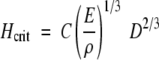
Young's modulus (E) is a crucial property in living plants as it affects their response to external and internal forces. E is defined as the ratio of the normal stresses to the normal strains measured within the proportional limit of loading of a linearly elastic material (Niklas, 1994). Density-specific stiffness, which is the quotient of E and density (ρ), can be used to predict the maximum height (H_crit) which trees can attain before buckling under self-weight by

(1)

where ρ is the density of green wood, D is stem diameter and C is a constant of proportionality (Greenhill, 1881). The safety factor defines the margin by which critical height exceeds actual height, H, and is defined as, H_crit/H.

If E/ρ and the safety factor remain constant with increases in D, eqn. 1 predicts that scaling of plant height (H) will be proportional to the 2/3 power of stem diameter (i.e. H ∝ D^2/3). This forms the basis for the elastic similarity model proposed by McMahon (1973) and McMahon and Kronauer (1976), and subsequently used to scale diameter with height in conifers and dicots (Dean and Long, 1986; Rich et al., 1986; Norberg, 1988; Bertram, 1989). However if E/ρ is not a constant, then the scaling exponent α for the proportional relationship H ∝ D^α depends on the scaling of E/ρ with D (Niklas, 1994). Although constant values for E/ρ are the basis for the elastic similarity model and are often assumed in calculations of critical heights (McMahon, 1973) and safety factors, to date the testing of this assumption has been mostly limited to a very broad level, investigating variation between genera (Niklas, 1993a, b) and between species (Niklas, 1994). While variation in E and E/ρ is known to occur along the lengths of individual tree trunks (Niklas, 1997), comparatively little is known about variation in E and E/ρ across conspecifics and how this variation is influenced by the environment.

Across a wide environmental range, theory suggests that E/ρ may be related to stem slenderness (S). When light-demanding species are grown under competition, rapid height growth is important to ensure that they are not overtopped by neighbours. Under high levels of competition, trees become etiolated as carbon is preferentially allocated to height growth at the expense of diameter increment. From eqn. 1 it can be seen that for a given E/ρ, actual height will approach the critical height as height for a given diameter, or slenderness, increases. Equation 1 shows that trees can increase their critical height to avoid buckling as slenderness increases by increasing their density-specific stiffness. As green density is relatively constant in young trees composed mainly of sapwood (Lasserre et al., 2005), this is accomplished primarily through increases in E.

The relationship between slenderness and E is more directly demonstrated by the following rearrangement of eqn. 1, in terms of the safety factor (H_crit/H) as;

(2)

Equation 2 shows that for a given diameter, increases in slenderness need to be accompanied by increases in E to maintain a constant safety factor.

Assuming that stem slenderness is the primary influence on E in stands growing under competition, other environmental factors will influence E in one of three ways (Fig. 1). The first mechanism of regulation would be a direct influence on E, independent of the influence of stem slenderness on E. Secondly, environmental factors could indirectly influence E through their direct influence on stem slenderness. Finally, they may exhibit both of the above influences, by directly influencing both E and stem slenderness.

Fig. 1.

Proposed causal pathways linking environmental variables with Young's modulus (E). Solid lines represent direct pathways of influence, while dashed lines represent indirect pathways of influence on E, via stem slenderness.

Linking the environment with wood properties at a broad scale requires detailed information on the climatic and edaphic conditions over a range of sites, at the time wood was laid down. This type of information is available from a nationwide series of environmental quality plots at sites encompassing the range of climatic and edaphic conditions found throughout plantations of the conifer Pinus radiata, within New Zealand (Watt et al., 2005a). At each location, trees were grown over a period of 4 years in plots with high stand density (spacing 0·5 × 0·5 m; 40 000 trees ha⁻¹) to ensure that material properties and stem geometry were governed by the need to avoid buckling through self-weight, rather than external forces such as wind. Using these data, the objectives of the study were to: (i) examine the range in E/ρ for trees growing across contrasting environments; (ii) determine how E/ρ, H_crit and the safety factor scales with D; and (iii) identify significant direct and indirect influences on E.

MATERIALS AND METHODS

Location of environmental quality plots

Sites were selected using Land Environment New Zealand (Leathwick et al., 2003) to encompass the widest possible range in environmental conditions on which P. radiata occurs within New Zealand (Fig. 2). Plots used within this study occur within the seven major soil orders on which 97·6 % of the P. radiata resource occurs. Sites were screened further using climatic surfaces (Leathwick and Stephens, 1998) to ensure that selected areas represented the considerable range in meteorological conditions found throughout New Zealand's planted forests. When compared with long-term average values for all plantation forests (Anonymous, 1983), meteorological data recorded at each location (Table 1) indicate that the 21 selected sites almost completely encompass the range in total annual rainfall (NZ plantations 609–3 718 mm vs. selected sites 457–3074 mm) and mean annual temperature (NZ plantations 8·0–15·6 °C vs. selected sites 8·6–15·3 °C).

Fig. 2.

Geographic distribution of the Land Environment New Zealand (LENZ) level I environments, showing the location of environmental quality plots used in this study.

Table 1.

Summary statistics for climatic variables, site attributes and soil properties

			Significance in path analysis
	Mean	Range	Direct effecton E	Direct effecton S
Climatic and site attributes
Mean annual air temperature (°C)	11·6	8·6–15·3	3·19*	2·75*
Mean March air temperature (°C)	14·5	10·9–17·9	3·68*	2·98*
Solar radiation (MJ PAR m−2)	5·6	4·1–6·8	ns	ns
Relative humidity (%)	84	68–92	ns	ns
Average windspeed (m s−1)	3·0	1·8–4·7	ns	ns
Rainfall (mm)	1493	457–3074	ns	ns
θa	0·69	0·36–0·89	–2·58*	ns
Root depth (m)	0·48	0·20–0·82	ns	2·78*
Average leaf area index (m2 m−2)	2·68	0·71–4·31	ns	3·82*
Chemical properties
Carbon (%)	6·0	1·7–26·7	ns	ns
Total N (%)	0·28	0·11–0·85	ns	ns
CN ratio	20	11–31	ns	ns
pH	5·1	4·1–6·0	ns	ns
CEC (cmol g−1)	19	9–43	ns	ns
Exch. Na (cmol g−1)	0·28	0–0·74	ns	2·18*
Exch. K (cmol g−1)	0·38	0·09–0·99	ns	ns
Exch. Mg (cmol g−1)	1·7	0·35–3·93	ns	ns
Exch. Ca (cmol g−1)	4·9	0·1–21·4	ns	ns
Base saturation (%)	36	8–94	2·04*	ns
Sum bases (cmol g−1)	7·4	1·1–20·8	ns	ns
Olsen P (μg g−1)	10	2–33	ns	ns
Bray P (μg g−1)	27	2–184	ns	ns
Inorganic P (mg g−1)	145	12–415	ns	ns
Organic P (mg g−1)	318	74–601	ns	ns
Total P (mg g−1)	463	914	ns	ns
Physical properties
Sand (%)	38	5–93	ns	1·97*
Silt (%)	40	4–71	ns	ns
Clay (%)	21	3–49	ns	ns
‘A’ horizon depth (m)	0·15	0·10–0·22	ns	ns
Bulk density (g cm−3)	0·96	0·47–1·35	2·50*	ns
Particle density (g cm−3)	2·5	2·2–3·0	3·1*	ns
Penetration resistance (MPa)	0·85	0·37–1·75	ns	ns
Total porosity (% v/v)	63	49–79	–2·23*	ns
Macroporosity (%)	21	7–49	ns	ns
Air capacity (%)	23	8–45	ns	ns

For each variable, the plot level mean and range is shown. Also shown is the significance for the direct effects of each variable on Young's modulus (E) and stem slenderness (S) when introduced into the initial path analysis model (see Fig. 1). Insignificance at the 5 % level is denoted by ns; where variables are significant at the 5 % level (t > |1·96|), the t-value is given.

Experimental design

Environmental quality plots were located at each of the 21 selected locations. While the trial series includes a wide range of treatments (see Watt et al., 2005a for full trial description), only those directly relevant to this study will be described. At each location, two plots of P. radiata were established, with one located on an undisturbed soil and the other on a disturbed soil compacted by previous harvesting operations. Samples were taken in the undisturbed treatment at all but three sites. At these three sites samples were taken from the disturbed plots as excessive mortality precluded use of the undisturbed plots.

Each plot was small in size (3 × 3 m) and contained nine measurement trees spaced at 0·5 m × 0·5 m (40 000 trees ha⁻¹) surrounded by a two-row buffer. Regular applications of herbicide were made to ensure weed-free conditions. All sites were planted with 1-year-old P. radiata seedlings with a growth and form factor of 19 (Vincent and Dunstan, 1989), sourced from the Scion nursery in Rotorua.

Measurements

Following the methods described in Watt et al. (2005a), a comprehensive set of soil physical properties was measured prior to planting. For consistency, all soil physical properties reported herein are averaged from 0 to 100 mm, except stone content and total available water content, which have been determined over the root depth, as measured at harvest.

Groundline diameter and height of the nine measurement trees were measured annually. Leaf area index, L_t, was measured every 4 months using a canopy analyser (LAI-2000, Li-Cor Inc., Lincoln, NE, USA). Measurements of photosynthetically active photon flux density, air temperature and relative humidity were taken from sensors installed on a 3 m tower located adjacent to the experimental plots. A tipping bucket rain gauge positioned on top of the tower was used to measure above-canopy rainfall. Annual average windspeed for each site was obtained from thin-plate spline surfaces (Hutchinson and Gessler, 1994) fitted to meteorological station data (Leathwick and Stephens, 1998).

A comprehensive set of soil chemical measurements was taken from the environmental quality plots after harvest at age 4 years. Soil chemistry samples were taken from 0 to 100 mm depth at 16 points in all harvested sub-plots to give 16 cores per bag. Sampling points were at least 0·5 m apart around nine trees at the centre of the plots. These samples were bulked by treatment then analysed for soil moisture, pH in water, total carbon (C), total soil nitrogen (N), total soil phosphorus (P), soil organic P, Bray P, Olsen P, exchangeable bases and CEC, following the methods described by Blakemore et al. (1987). Results are expressed on an oven-dry basis (105 °C).

At age 4 years, trees were extracted from the ground when groundline diameter averaged 46 mm and height averaged 3·7 m (Table 2). Plot-level estimates of root depth were determined by measuring the depth of the deepest root on five trees per plot. A 300 mm section of the stem centred around 10 % of the total tree height was cut from each tree, stored on ice and transported back to the laboratory.

Table 2.

Summary statistics for tree dimensions at harvest (age 4), and modulus of elasticity (E)

Variable	Mean	Range
Height (m)	3·7 (0·2)	0·9–5·9
Diameter (mm)	46 (2)	17–60
Slenderness (m m−1)	82 (4)	52–109
E (GPa)	4·4 (0·3)	2·3–6·9

For each variable, the plot level mean ± s.e. and range from 21 sites are shown.

In the laboratory, bark was removed from the stem sections. Green density (ρ) was then determined on the stem section as green weight/green volume. Green volume was determined on the whole stem section using the immersion technique. Following Evans and Ilic (2001), green dynamic Young's modulus (E _d) was determined on the whole stem section from measurements of green density ρ and sound velocity V, using the following equation;

(3)

Sound velocity was measured by the resonance-based tool, Woodspec (Industrial Research, Lower Hutt, New Zealand). This tool uses the impact from a pendulum to generate a stress wave within the wood sample. As the stress wave must travel twice the length of the sample during one oscillation cycle, the velocity of the wave is given by, V = 2lf, where f is the fundamental resonance frequency and l is the sample length. Young's modulus was measured using this method as it is fast and provides accurate estimates of E. In a recent study using material from 4-year-old P. radiata clones, Lindström et al. (2002) found the correspondence between dynamic modulus of elasticity measured using resonance and traditional static bending (E_s) to be very strong (r² = 0·98) and linearly related as E_d = 1·04 E_s.

Determination of water balance

Fractional available root-zone volumetric water content, θ_a, on day i was determined at all 21 sites using the water balance model described in Appendix. During the fourth year after planting, monthly gravimetric measurements of root-zone volumetric water content, θ, were made to a depth of 300 mm at three sites subject to seasonal water deficits. Using eqn. A6 (see Appendix) and site-specific measurements of mimimum and maximum θ (see Appendix for details), values of θ_a were determined for the gravimetric samples. Modelled values of θ_a exhibited good correspondence with the seasonal gravimetric measurements at each site. Average absolute differences between measured and modelled θ_a at the three sites were 1, 8 and 3 %, respectively.

Data analysis

All analyses were undertaken in SAS (SAS Institute, 1996), using plot-level data. Allometric analysis was used to examine relationships between H_crit, E, E/ρ, H, D and S at age 4. Plot-level stem slenderness (S) was determined as the average of tree level values, calculated as H/D. Critical height was determined by eqn. 1, using a value for C of 0·792 (Niklas, 1994). For dimensional consistency within eqn. 1, all values for E/ρ herein are expressed in units of m, by converting ρ into Newtons m⁻³ (i.e. 1 kg weight force = 9·8067 N).

Regression models of the form

(4)

were used to determine the parameters α and β for the allometric relationships. Reduced major axis (RMA) regression analyses were used to determine the scaling exponents and allometric constants (i.e. α_RMA and logβ_RMA, respectively) for the logY vs. logX allometric trends observed because the objective was to determine functional rather than predictive relationships. These two regression parameters were computed using the formulas α_RMA = α_OLS/r and logβ_RMA = − α_RMA , where α_OLS is the ordinary least squares (OLS) regression exponent, r is the OLS correlation coefficient and , denote mean values of variables logY and logX, respectively (Sokal and Rohlf, 1981; Niklas, 1994; Niklas et al., 2006). Determination of 95 % confidence intervals (CIs) for α_RMA and logβ_RMA was undertaken using the formulas 95 % CI = α_RMA ± t_N-2 (MSE/SS_X)^1/2 and 95 % CI = logβ_RMA ± t_N-2 {MSE[(1/n) + (²/SS_X)]}^1/2, where MSE is the OLS regression model mean square error, SS_X is the OLS sums of squares and n is sample size (Sokal and Rohlf, 1981; Niklas, 1994; Niklas et al., 2006).

The influence of environment on E was analysed by both regression analysis and path analysis, using the independent variables listed in Table 1. Average leaf area index over the study period was used in the analysis as a competition index for light as, according to Beers Law, above-canopy available flux density reaching the soil surface exponentially declines with increasing leaf area index (see eqn. A5, in Appendix). All climatic variables used in the analysis, including θ_a, were averaged over the entire 4 year period, from daily values, except total rainfall, which was averaged over yearly sums for the 4 year period. Values of stem slenderness used in the analysis were measured at age 4. Prior to analysis, all variables were tested for normality and homogeneity of variance and transformations made as necessary to meet the underlying statistical assumptions of the models used.

Univariate relationships between E and all independent variables were examined, using appropriate functional forms to determine which variables were significantly related to E. Although regression analysis provides useful information of the strength and form of relationships, it does not separate indirect from direct effects.

To control for the effects of common cause, path analysis was used as an extension to regression analysis, using the CALIS procedure (SAS Institute, 1996). The path analysis method, which is briefly outlined in Appendix, is more fully described in Wright (1921, 1934), Li (1975) and Rao and Morton (1980). The direct and indirect effects, through stem slenderness, of all edaphic and climatic pathways on E, was tested by introducing them singly into the model outlined in Fig. 1. The final model was developed by introducing all those variables previously found to have significant direct effects into the model sequentially, starting with the variables most strongly related to stem slenderness and E. Variables were retained if pathways were significant, and they significantly reduced the chi-square of the overall model (see Appendix for details). The tests used to determine variable significance and overall model fit are given in Appendix.

RESULTS

Site-level variation in measured variables

Between-site variation in height, diameter and stem slenderness at age 4 was substantial and highly significant (P < 0·001) for all variables (Table 2). Plot-averaged values varied 7-fold for height (0·9–5·9 m), 4-fold for diameter (17–60 mm) and 2-fold for stem slenderness (52–109 m m⁻¹). At age 4, within-plot tree height was very homogenous as evidenced by the low within-plot standard error which averaged 9 % of the mean across the 21 sites. Within-site variation in diameter and stem slenderness was also low, with standard errors averaging 6 and 5 %, respectively, of the mean value for these variables. Average leaf area index exhibited 6-fold variation across sites, ranging from 0·71 to 4·31 m² m⁻².

Climatic variation between sites was considerable (Table 1). Across sites, average fractional available volumetric water content (θ_a) ranged from 0·36 on a dryland site (site 19; Fig. 2) with very low annual average rainfall (457 mm) to 0·89 on a wet west coast site (site 16; Fig. 2) with very high average annual rainfall of 3074 mm. Average temperature exhibited a 2-fold variation from 8·6 °C at a high elevation South Island site (site 19; Fig. 2) to 15·3 °C at a coastal site (site 3; Fig. 2) in the northern North Island.

The selected sites included extremes in soil texture ranging from single-grained scoria and sandy soils to clay loam soils. Variation in soil texture was considerable for all classes (Table 1) and most pronounced for the sand (5–93 %) and silt fractions (4–71 %). Soil physical properties also exhibited considerable variation between sites. This variation was most pronounced for the closely related variables macroporosity and air capacity which ranged from 7 to 49 % and from 8 to 45 %, respectively, across sites.

All chemical properties exhibited substantial variation between sites (Table 1). Site variation was most marked for exchangeable calcium, Bray P, inorganic P and sum of bases, which exhibited respective ranges of 153-, 108-, 35- and 19-fold across sites. Exchangeable Na also showed a considerable site range from 0 to 0·74 cmol g⁻¹.

Allometric scaling relationships and variation in E/ρ

Young's modulus exhibited a highly significant (P < 0·001) 3-fold variation between sites, with plot-averaged values ranging from 2·3 to 6·3 GPa (Table 2). Within-plot variation in E was low, with standard errors averaging 9 % of the mean value, across the 21 plots. As plot-averaged green density exhibited only a 5 % range (1080–1144 kg m⁻³), density-specific stiffness also varied 3-fold across sites (207 678–635 670 m), and exhibited a strong (r² = 0·999) positive isometric relationship with E (Table 3).

Table 3.

Summary statistics of reduced major axes (RMA) regression of logY vs. logX

Variable
logY	logX	αRMA	logβRMA	r2
E/ρ	E	1·00 (0·98–1·02)	4·96 (4·95–4·97)	0·99
Hcrit	D	0·95 (0·79–1·11)	2·14 (1·93–2·36)	0·89
(E/ρ)0.33	D	0·39 (0–0·78)	2·39 (1·87–2·91)	0·35
E/ρ	S	1·43 (1·17–1·70)	2·88 (2·38–3·37)	0·71
H	D	1·63 (1·44–1·82)	2·74 (2·48–3·00)	0·85

The scaling exponent (α_RMA) and allometric constant (logβ_RMA) are presented with 95 % confidence intervals in parentheses.

Regression of critical buckling height against diameter (Fig. 3A) yielded a scaling exponent of 0·95. This scaling exponent was higher than the exponent of 0·67 predicted with constant E/ρ by eqn. 1, as (E/ρ)^1/3 scaled with D to the power of 0·39. The scaling exponent between actual height, H, and D was 1·63 (Table 3; Fig. 3A). E/ρ scaled positively with stem slenderness to the power of 1·43. The safety factor, which ranged from 1·61 to 3·50, declined with increasing values of D (Fig. 3A) and stem slenderness (Fig. 3B).

Fig. 3.

(A) Log–log (base 10) plot of groundline diameter against estimated critical buckling height (filled circles) and actual height (open circles), with RMA regression curves (see Table 3 for parameters) shown as a solid line for H_crit, and a dotted line for H. (B) Relationship between the safety factor (H_crit/H) and stem slenderness.

Univariate relationships with Young's modulus

In total, E was significantly related to 11 variables. Variables exhibiting the five strongest significant univariate relationships in order of descending strength were stem slenderness (r² = 0·59; P < 0·001), tree height (r² = 0·54; P < 0·001), mean annual air temperature (r² = 0·52; P < 0·001), average θ_a (r² = 0·33; P < 0·05) and leaf area index (r² = 0·32; P < 0·01). The correlation between E and average annual rainfall was not significant.

When examined at the monthly level, the strongest relationship between E and mean temperature (Fig. 4A) occurred in March (T_aut) during early autumn (r² = 0·58). There were positive linear relationships between E and both stem slenderness (Fig. 4B) and leaf area index. The relationship between E and average fractional available volumetric water content (θ_a) was peaked, with maximum values of E occurring at θ_a values of 0·70 (Fig. 4C).

Fig. 4.

Relationship between Young's modulus (E) and (A) average temperature during March (B) stem slenderness and (C) average fractional available volumetric water content (θ_a).

Development of a model partitioning indirect and direct influences on Young's modulus

The direct and indirect (through stem slenderness) effects of all edaphic and climatic variables on E were tested, by introducing them singly into the model (Fig. 1). As path analysis requires linear relationships between variables, θ_a was transformed so it exhibited linear relationships with E and stem slenderness by calculating absolute differences from the optimum value. The optimum value of 0·64 for θ_a was empirically determined as the value across the range of θ_a (0·36–0·89) which minimized the mean square error for differences between measured and modelled values.

Results show that mean air temperature in March (T_aut) had the strongest significant (P < 0·05; t-value = 3·68) direct association with E, surpassing the significant (P < 0·05; t-value = 3·19) association of mean annual air temperature with E (Table 1). Other variables which had significant (P < 0·05) direct associations with E in order of descending strength were particle density, θ_a, bulk density, total porosity and base saturation. Variables which exhibited significant (P < 0·05) direct associations with stem slenderness, thereby indirectly influencing E, in order of descending strength included leaf area index, T_aut, root depth, mean annual air temperature, exchangeable Na and sand content.

To develop a final model, variables significantly related to E and stem slenderness were introduced into the model sequentially in order of importance, and were retained if they were found to have a significant effect on either E or stem slenderness. Following this process, the final model is outlined in Fig. 5. The only variables found to have a significant direct association with E were T_aut and stem slenderness, and the only variables which were significantly directly associated with stem slenderness were T_aut and leaf area index (Fig. 5). As the covariance between T_aut and leaf area index was not significant (P = 0·11), this pathway was dropped. For the final model, an acceptable level of model fit to the data was demonstrated by all goodness of fit indices (all >0·9) and the chi-square ratio (P = 0·55). None of the normalized residuals exceeded 0·59 in absolute magnitude. In addition, all pathways in the final model were non-trivial in magnitude (path coefficients >0·3).

Fig. 5.

Final path analysis model, with significant (P < 0·05) pathways shown. Solid lines represent direct pathways of influence, while dashed lines represent indirect pathways of influence. Values next to each line give the path coefficient for that pathway. The amount of variance (r²) explained for each endogenous variable is shown.

The positive direct influence of leaf area index on stem slenderness was stronger than the positive direct influence of T_aut on stem slenderness (0·51 vs. 0·36). The direct effects of stem slenderness and T_aut on E were both positive and of a similar magnitude (0·50 vs. 0·49). Total effects, which include both the direct and indirect pathways, indicate that E was most sensitive to changes in T_aut (0·44), followed by stem slenderness (0·37) and then leaf area index (0·35). The final model explained 76 % of the variance in E and 53 % of the variance in stem slenderness.

DISCUSSION

Results from this study show variation in E/ρ for P. radiata to be very significant and substantial, ranging 3-fold, when trees were grown under competition across diverse environments. Although most of the variation in E/ρ was attributable to slenderness, the density-specific stiffness term in eqn. 1 [(E/ρ)^1/3] did scale positively with diameter to the power of 0·39. Consequently, the relationship between critical height and D, scaled to the power of 0·95, which considerably exceeds the value for α of 0·67 used when E/ρ is assumed to be constant.

Although the scaling exponent between H_crit and D was higher than predicted (0·95 vs. 0·67), H_crit/H still declined with increases in D, violating the assumption of constant safety margins which form the basis of the elastic similarity model. While previous research has shown young trees to have a higher scaling exponent between H and D than mature trees (Whittaker and Woodwell, 1968), values of α reported in this study exceed all previously reported values for trees (Whittaker and Woodwell, 1968; Niklas 1993a), and do not conform to either the elastic similarity model (α = 0·67) or the model of geometric similarity (α = 1).

The high scaling exponent between H and D occurred as the very high 7-fold variation in height at age 4 across the site gradient was accompanied by a lower 4-fold variation in diameter. Results from the path analysis show that these resulting 2-fold increases in stem slenderness, across the range in D, were primarily associated with increases in leaf area index and, to a lesser extent, air temperature. Given that radiation reaching lower canopy layers exponentially declines with increasing leaf area index, the positive relationship between leaf area index and slenderness strongly suggests that trees become more etiolated as competition for light increases on more productive sites with high D. This response is consistent with previous research (Albrekston and Valinger, 1985; Nilsson and Albrekston, 1993; Vanninen and Mäkelä, 2000), and likely to be a survival mechanism whereby greater carbon allocation to height growth under high levels of shading enables trees to avoid being overtopped.

The results suggest that reductions in the safety factor, associated with increases in slenderness, induced increases in E/ρ to reduce the risk of stem buckling. The strong inverse relationship found between slenderness and the safety factor was not surprising as slenderness is the dominant term in eqn. 2, and the scaling exponent between (E/ρ)^1/3 and D (0·39) gave a product between these two variables in eqn. 2 (E/ρ^1/3D^−1/3) which was close to dimensionless. Although the positive scaling between E/ρ and slenderness did not maintain the safety factor at a constant value, increases in E/ρ nonetheless imparted greater stability than would have been present had E/ρ remained constant with increasing slenderness. Constant safety margins have been found for relatively open grown mature trees on different sites (Niklas 1994). Results from this study suggest this constancy will not hold for young densely grown plantation species occurring across diverse environments, as increases in stem slenderness induced by higher competition for light are not sufficiently offset by increases in E.

The mechanism by which slenderness affects E was not explicitly examined in this study. However, it can be shown that for a given mass, a more slender tree will have a greater level of compressive stress in its stem (Niklas, 1994, p. 164). It is hypothesized that trees are able to sense and respond to this higher level of compressive stress and produce new wood with higher E, possibly by manipulating the angle of cellulose microfibrils in the secondary cell wall. This increase in E not only acts to reduce the compressive strains experienced by the stem, but in turn also acts to increase the critical compressive stress that the tree stem can withstand before buckling occurs. This type of thigmomorphogenic response to mechanical stresses caused by self-imposed or dynamic loads commonly occurs in a large number of tree species (Jaffe, 1973), including P. radiata (Jacobs, 1954).

From the path analysis model, air temperature also exhibited a significant association with E and by inference E/ρ, as it influences these two properties both directly and indirectly through slenderness. The significant direct influence of air temperature on E may be mediated through regulation of latewood development. Analyses show that E was most strongly correlated with mean temperature during early autumn. Given that latewood with high E is forming during this period (Watt et al., 2005b), it follows that sites with warmer temperatures and increased growth rates over this month will develop a greater percentage of high E latewood, and as a consequence higher overall stem E.

The effects of wind on tree morphology (Jacobs, 1954; Telewski and Jaffe, 1986a, b; Telewski, 1989) and biomechanical properties (Nicholls, 1982; Telewski and Jaffe, 1986a; Pruyn et al., 2000) have been well documented; however, wind speed did not significantly influence either morphology or E in our study. Trees within this study were planted at a very high stand density, where crowns were in contact at almost all sites from the second year onwards. Previous research shows that high stand densities lower stem deflection through both reducing wind speed within the canopy (Raupach, 1992; Green et al., 1995) and damping stem oscillations through increasing the number of collisions with neighbours (Milne, 1991). As a result, it is likely that both morphology and E of trees inside the buffer rows responded more to self-load than to external forces such as wind. This is supported by the absence of a significant correlation between wind speed and either slenderness or E.

While the safety factors found in this study were comparatively low, they did exceed unity, which is consistent with field observations as buckling was not found throughout the trial series. It is likely that the relatively low safety factors (average of 2·1) found in this study were attributable to the high stand densities indicative of plantation-grown trees, which have a more unstable etiolated form than open grown trees. Our values were consistent with safety factors reported for 9-year-old sweet gum growing under competition which exhibited a similar range of slenderness ratios to trees in our study, reaching maximum values of 116 m m⁻¹ (Holbrook and Putz, 1989).

Many of the key results presented herein and the inferences drawn from them are based on the Euler column formula. Care is required when applying this formula as it assumes that columns are perfectly straight and uniform in cross-section throughout their length. They must also be constructed from an isotropic material, i.e. they must have a uniform E in the longitudinal and radial directions, and the weight of the column must be significantly less than the weight that it supports. Clearly, tree stems do not conform to these ideal conditions. Young's modulus varies in the longitudinal and radial directions, tree diameter declines with increasing height, and the weight of the stem typically exceeds the loads that they must support (i.e. the mass of the crown, which itself is generally not axisymmetric). Nonetheless, the Euler column formula provides a useful tool for examining the relationship between tree slenderness and E.

In summary, the results indicate that constant E/ρ cannot be assumed for plantation-grown P. radiata growing across an environmental gradient. As E/ρ scales positively with D, the scaling exponent found between D and H_crit of 0·95 exceeds the value of 0·67 assumed under constant E/ρ. Although the scaling exponent between H_crit and D was higher than predicted, convergence between H_crit and H was still observed as D increased. The results suggest that reductions in the safety factor, associated with increases in slenderness, induced increases in E/ρ and E to reduce the risk of stem buckling. Air temperature was also found to be significantly associated with E both directly and indirectly through its influence on slenderness. Models such as the one developed in this study may provide a basis for estimating within-species E, E/ρ and H_crit across environmental gradients.

APPENDIX

Water balance model

A daily water balance equation was used to calculate root zone water storage (W) on the ith day as

(A1)

where P_i is rainfall, E_ti is transpiration from the dry tree canopy, E_twi evaporation of intercepted rainfall from the tree canopy, E_gi evaporation from the soil, and F_i drainage from the root zone (Whitehead et al., 2001).

Transpiration from the tree canopy was calculated using the simple diffusion equation

(A2)

where D_a is the air saturation deficit, g_st is the average stomatal conductance for the canopy, L_t is the projected leaf area index, and φ will be defined later. The inverse relationship between stomatal conductance and air saturation deficit was modelled using the function described by Lohammer et al. (1980) as

(A3)

where g_stmax describes maximum stomatal conductance at low air saturation deficit, and D₀ is the sensitivity of g_st to D_a, when D_a > D_smin.

E_g was calculated from the available energy beneath the tree canopy, G_g, as,

(A4)

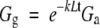
where the coefficient τ (=1·4) describes the degree of coupling of the soil surface with the air above the canopy (Kelliher et al., 1990), s is the slope of the relationship between saturated vapour pressure and temperature at a given air temperature, λ is the latent heat of vaporization, γ is the psychometric constant, and φ will be defined later. Values for s, γ and λ are temperature dependent and calculated from standard meteorological tables. Using Beers Law, G_g was calculated from

(A5)

where G_a is the available flux density above the canopy (assumed to be 70 % of shortwave radiation) and k is the light extinction coefficient (assumed to be 0·5 for a spherical leaf angle distribution).

The coefficient φ was used to reduce evaporation from the soil and transpiration as soil water storage declined. Root zone volumetric water content on the ith day, θ_i {=W_i/[d(1−c)]}, was calculated from water storage in the profile (W_i), root zone depth (d) and fractional stone content of the soil (c). The value of the coefficient φ was set to 1 at maximum values of θ (θ_max), and was not reduced until θ declined to a threshold value (θ_t). As θ progressively declined below this threshold, φ was linearly reduced from 1 to 0 at minimum values of θ (θ_min). The threshold values (θ_t) for reducing evaporation from the soil and transpiration, taken from Watt et al. (2003), were assumed to be respectively 60 and 55 % of fractional available volumetric water content, θ_a, determined as,

(A6)

Evaporation from the soil and transpiration were reduced to 50 % of their potential rates on days when rain fell. Drainage from the root zone was assumed to be zero when θ_i ≤ θ_max and equal to rainfall reaching the soil when θ_i > θ_max.

Daily meteorological data required for the water balance model include total rainfall and solar radiation, mean air temperature and average air saturation deficit. Parameter values for g_stmax, D₀ and D_smin were assumed to be 0·15 mmol⁻² s⁻¹, 0·94 kPa and 0·5 kPa, respectively. As previously described, values of root depth (d) and stone content (c) were measured at each site. Following Gradwell (1972), θ_max and θ_min were determined at each site from soil in the top 100 mm at tensions of 10 and 1500 kPa, respectively. L_t was modelled at a daily level by interpolating between seasonal measurements using a spline function. Following Landsberg and Waring (1997), wet canopy evaporation as a percentage of daily rainfall, P, was assumed to increase linearly from 0 at L_t of 0 to (0·15P) at L_t of 3, after which there were no further increases.

Path analysis

Path analysis is a multivariate statistical technique which bridges the gap between empirical observation and theoretical research. This technique requires development of a preconceived causal model in which directional flow and the inter-relationships among independent (exogenous) and dependent (endogenous) variables are specified. In contrast, regression analysis maximizes the prediction of dependent variables from independent variables with no ‘cause and effect’ implication. Thus, path analysis provides both flexibility and greater insights into causal structure than regression analysis.

A comprehensive range of tests was used to determine the significance of the pathways and final model fit. The significance of pathways between exogenous and endogenous variables in the causal model was assessed to ensure that they were significant at the 5 % level (absolute t-value >1·96), and non-trivial in magnitude (path coefficient >0·3). For the overall model, values of the chi-square ratio >0·05 indicate an acceptable fit between model and data. However, as the chi-square statistic has some limitations as an inferential test (see Kaplan 1990, for a review), the goodness of fit index, normed fit index and comparative fit index (CFI) were also used to determine the adequacy of the model fit to the data. All of these indices range from 0 to 1, with values >0·9 indicating an acceptable fit between model and data. A model exhibiting acceptable fit between the model and the data also has normalized residuals which are <2·00.

For the final model, the magnitude of the standardized coefficient, which ranges from 0 to 1, was examined to evaluate the relative importance of relationships between the exogenous and endogenous variables. As the standardized coefficients indicate the fraction of a unit change in standard deviation of the response variable for a one unit change in standard deviation of the driving variable, values closer to 1 indicate a greater degree of influence. The total effects, which include both the direct and indirect pathways for each driving variable, were also examined.

LITERATURE CITED

- Albrekston A, Valinger E. 1985. Relations between tree height and diameter, productivity and allocation of growth in Scots pine (Pinus sylvestris L.) sample tree material. In: Tigerstedt PMA, Puttonen P, Koski, V, eds. Crop physiology of forest trees. Finland: University of Helsinki, 95–105.
- Anonymous. 1983. Summaries of climatological observations to 1980. Wellington, New Zealand: New Zealand Meteorological Service Miscellaneous Publication 177.
- Bertram JEA. 1989. Size-dependent differential scaling in branches: the mechanical design of trees revisited. Trees 4: 241–253. [Google Scholar]
- Blakemore LC, Searle PL, Daly BK. 1987. Methods for chemical analysis of soils. Wellington, New Zealand: Department of Scientific and Industrial Research. New Zealand Soil Bureau Scientific Report No. 80.
- Dean TJ, Long JN. 1986. Validity of the constant-stress and elastic instability principles of stem formation in Pinus contorta and Trifolium pratense. Annals of Botany 58: 833–840. [Google Scholar]
- Evans R, Ilic J. 2001. Rapid prediction of wood stiffness from microfibril angle and density. Forest Products Journal 51: 53–57. [Google Scholar]
- Gradwell MW. 1972. Methods for physical analysis of soils. Wellington, New Zealand: Department of Scientific and Industrial Research. New Zealand Soil Bureau Scientific Report No. 10C.
- Green SR, Grace J, Hutchings NJ. 1995. Observation of turbulent air flow in three stands of widely spaced Sitka spruce. Agricultural and Forest Meteorology 74: 205–225. [Google Scholar]
- Greenhill AG. 1881. Determination of the greatest height consistent with stability that a vertical pole or mast can be made, and of the greatest height to which a tree of given proportions can grow. Proceedings of the Cambridge Philosophical Society 4: 65–73. [Google Scholar]
- Holbrook NM, Putz FE. 1989. Influence of neighbours on tree form: effects of lateral shade and prevention of sway on the allometry of Liquidamber styrafaciflua (Sweet gum). American Journal of Botany 76: 1740–1749. [Google Scholar]
- Hutchinson MF, Gessler PE. 1994. Splines—more than just a smooth interpolator. Geoderma 62: 45–67. [Google Scholar]
- Jaffe MJ. 1973. Thigmomorphogenesis: the response of plant growth and development to mechanical stress. Planta 114: 143–157. [DOI] [PubMed] [Google Scholar]
- Jacobs MR. 1954. The effect of wind sway on the form and development of Pinus radiata D. Don. Australian Journal of Botany 2: 35–51. [Google Scholar]
- Kaplan D. 1990. Evaluating and modifying covariance structure models: a review and recommendation. Multivariate Behavioural Research 25: 137–155. [DOI] [PubMed] [Google Scholar]
- Kelliher FM, Whitehead D, McAneney KJ, Judd MJ. 1990. Partitioning evapotranspiration into tree and understorey components in two young Pinus radiata D. Don stands. Agricultural and Forest Meteorology 50: 211–227. [Google Scholar]
- Landsberg JJ, Waring RH. 1997. A generalised model of forest productivity using simplified concepts of radiation-use efficiency, carbon balance and partitioning. Forest Ecology and Management 95: 209–228. [Google Scholar]
- Lasserre JP, Mason EG, Watt MS. 2005. The effects of genotype and spacing on Pinus radiata [D.Don] corewood stiffness in an 11 year old experiment. Forest Ecology and Management 205: 375–383. [Google Scholar]
- Leathwick JR, Stephens RTT. 1998. Climate surfaces for New Zealand. Lincoln, New Zealand: Landcare Research Contract Report LC9798/126.
- Leathwick J, Wilson G, Rutledge D, Wardle P, Morgan F, Johnston K, et al. 2003. Land environments of New Zealand. Auckland, New Zealand: David Bateman Ltd.
- Li CC. 1975. Path analysis—a primer. London: Boxwood Press.
- Lindström H, Harris P, Nakada R. 2002. Methods for measuring stiffness of young trees. Holz als Roh und Werkstoff 60: 165–174. [Google Scholar]
- Lohammer T, Larsson S, Linder S, Falk SO. 1980. FAST—simulation models of gaseous exchange in Scots pine. Ecological Bulletin 32: 505–523. [Google Scholar]
- McMahon TA. 1973. Size and shape in biology. Science 179: 1201–1204. [DOI] [PubMed] [Google Scholar]
- McMahon TA, Kronauer RE. 1976. Tree structures: deducing the principle of mechanical design. Journal of Theoretical Biology 59: 443–466. [DOI] [PubMed] [Google Scholar]
- Milne R. 1991. Dynamics of swaying of Picea sitchensis. Tree Physiology 9: 383–399. [DOI] [PubMed] [Google Scholar]
- Nicholls JWP. 1982. Wind action, leaning trees and compression wood in Pinus radiata D. Don. Australian Forest Research 12: 75–91. [Google Scholar]
- Niklas KJ. 1993a. The scaling of plant height: a comparison among major plant clades and anatomical grades. Annals of Botany 72: 165–172. [Google Scholar]
- Niklas KJ. 1993b. Influence of tissue density-specific mechanical properties on the scaling of plant height. Annals of Botany 72: 173–179. [Google Scholar]
- Niklas KJ. 1994. Plant allometry—the scaling of form and process. Chicago, IL: University of Chicago Press.
- Niklas KJ. 1997. Mechanical properties of black locust (Robinia pseudoacacia L.) wood. Size and age-dependent variations in sap- and heartwood. Annals of Botany 79: 265–272. [Google Scholar]
- Niklas KJ, Cobb ED, Marler T. 2006. A comparison between the record height-to-stem diameter allometries of Pachycaulis and Leptocaulis species. Annals of Botany 97: 79–83. [DOI] [PMC free article] [PubMed] [Google Scholar]
- Nilsson U, Albrekston A. 1993. Productivity of needles and allocation of growth in young Scots pine of different competitive status. Forest Ecology and Management 62: 173–187. [Google Scholar]
- Norberg RÅ. 1988. Theory of growth geometry of plants and self-thinning of plant populations: geometric similarity, elastic similarity, and different growth modes of plant parts. American Naturalist 131: 220–256. [Google Scholar]
- Pruyn ML, Ewers BJ III, Telewski FW. 2000. Thigmomorphogenesis: changes in the morphology and mechanical properties of two Populus hybrids in response to mechanical perturbation. Tree Physiology 20: 535–540. [DOI] [PubMed] [Google Scholar]
- Rao DC, Morton NE. 1980. Path analysis of quantitative inheritance. In: Meieke JH, Crawford MH, eds. Current developments in antropological genetics vol 1. Theory and methods. New York: Plenum Press, 355–372.
- Raupach MR. 1992. Drag and drag partition on rough surfaces. Boundary-Layer Meteorology 60: 375–395. [Google Scholar]
- Rich PM, Helenurm K, Kearns D, Morse SR, Palmer MW, Short L. 1986. Height and stem diameter relationships for dicotyledonous trees and arborescent palms of Costa Rica tropical wet forest. Bulletin of the Torrey Botanical Club 113: 241–246. [Google Scholar]
- SAS Institute. 1996. SAS/STAT software: changes and enhancements through release 6.11. Cary, NC: SAS Institute Inc.
- Sokal RR, Rohlf FJ. 1981. Biometry, 2nd edn. New York, NY: W. H. Freeman.
- Telewski FW. 1989. Structure and function of flexure wood in Abies fraseri. Tree Physiology 5: 113–122. [DOI] [PubMed] [Google Scholar]
- Telewski FW, Jaffe MJ. 1986a. Thigmomorphogenesis: field and laboratory studies on Abies fraseri in response to wind or mechanical perturbation. Physiologia Plantarum 66: 211–218. [DOI] [PubMed] [Google Scholar]
- Telewski FW, Jaffe MJ. 1986b Thigmomorphogenesis: anatomical, morphological and mechanical analysis of genetically different sibs of Pinus taeda in response to mechanical perturbation. Physiologia Plantarum 66: 219–226. [DOI] [PubMed] [Google Scholar]
- Vanninen P, Mäkelä A. 2000. Needle and stem wood production in Scots pine (Pinus sylvestris) trees of different age, size and competitive status. Tree Physiology 20: 527–533. [DOI] [PubMed] [Google Scholar]
- Vincent TG, Dunstan JS. 1989. Register of commercial seedlots issued by the New Zealand Forest Service. Rotorua, New Zealand: Ministry of Forestry, Rotorua. Forest Research Institute Bulletin No. 144, Forest Research Institute.
- Watt MS, Whitehead D, Richardson B, Mason EG, Leckie AL. 2003. Modelling the influence of weed competition on the growth of young Pinus radiata at a dryland site. Forest Ecology and Management 178: 271–286. [Google Scholar]
- Watt MS, Coker G, Clinton PW, Davis M, Parfitt R, Simcock R, et al. 2005a. Defining sustainability of plantation forests through identification of site quality indicators influencing productivity—a national view for New Zealand. Forest Ecology and Management 216: 51–63. [Google Scholar]
- Watt MS, Downes GM, Whitehead D, Mason EG, Richardson B, Grace JC, et al. 2005b. Wood properties of juvenile Pinus radiata growing in the presence and absence of competing understory vegetation at a dryland site. Trees: Structure and Function 19: 580–586. [Google Scholar]
- Whitehead D, Leathwick JR, Walcroft AS. 2001. Modeling annual carbon uptake for the indigenous forests of New Zealand. Forest Science 47: 9–19. [Google Scholar]
- Whittaker R, Woodwell GM. 1968. Dimension and reproduction relations of trees and shrubs in the Brookhaven Forest, New York. Journal of Ecology 56: 1–25. [Google Scholar]
- Wright S. 1921. Correlation and causation. Journal of Agricultural Research 20: 557–587. [Google Scholar]
- Wright S. 1934. The method of path coefficients. Annals of Mathematical Statistics 5: 161–215. [Google Scholar]