Robust Estimation of Spatially Variable Noise Fields

Abstract

Consideration of spatially variable noise fields is becoming increasing necessary in magnetic resonance imaging given recent innovations in artifact identification and statistically-driven image processing. Fast imaging methods enable study of difficult anatomical targets and improve image quality but also increase the spatial variability in the noise field. Traditional analysis techniques have either assumed that the noise is constant across the field of view (or region of interest) or have relied on separate magnetic resonance image acquisitions to measure the noise field. These methods are either inappropriate for many modern scanning protocols or are overly time-consuming for already lengthy scanning sessions. We propose a new, general framework for estimating spatially variable noise fields from related, but independent magnetic resonance scans which we call noise field equivalent scans. These heuristic analyses enable robust noise field estimation in the presence of artifacts. Generalization of noise estimators based on uniform regions, difference images, and maximum likelihood are presented and compared with the estimators derived from the proposed framework. Simulations of diffusion tensor imaging and T2-relaxometry demonstrate a ten-fold reduction in mean squared error in noise field estimation, and these improvements are shown to be robust to artifact contamination. In vivo studies show that spatially variable noise fields can be readily estimated with typical data acquired at 1.5T.

Introduction

In many scenarios, noise cannot be ignored in the measurement of and computation from magnetic resonance (MR) images. For example, in some parts of the body (e.g., spinal cord, optic nerve) or when using certain pulse sequences (e.g., magnetic resonance spectroscopy), the signal obtained is on the same order as the noise. As well, the detrimental impacts of noise can be amplified when computing quantities of interest (e.g., diffusion contrasts) from the observed signals. Therefore, if image-based properties are to be measured and computed with a known degree of certainty, it is prudent to study the properties of noise in an MRI experiment and to understand how its effects can be characterized and ultimately mitigated.

Fast imaging methods, including multiple-element coils coupled to parallel imaging reception and reconstruction, enable the study of difficult anatomical tissues and can improve image quality; but these methods also increase the spatial variability of the noise. Traditional noise analysis techniques have either assumed that the noise is constant (i.e., spatially invariant) within the field of view or region of interest [7,10,12,15,16,23–25] or have relied on separate MRI acquisitions to accurately characterize the spatial variation of the noise [6,13]. The assumption of a spatially invariant noise is not well founded given both that modern MRI protocols use multiple array receive coils and that image tissues have spatially distributed compositions. But the use of extra scans for noise field mapping is rarely practiced because of imaging time constraints; furthermore, such scans are generally not available for the retrospective analysis of existing datasets [13]. The challenge of estimating spatially varying noise is further confounded by both the paucity of repeated acquisitions from which one can extract measures of reproducibility as well as the prevalence of heterogeneous imaging artifacts, which do not follow well-described distributions in MR images. We propose a new, general framework for estimating spatially variable noise fields (SVNFs) from related, but independent MR scans. These data are commonly acquired during the course of sensitized sequences in which weighted images are compared to reference images (e.g., diffusion tensor imaging (DTI) [1], T1/T2 relaxometry [9], functional MRI [21], magnetization transfer [20], and arterial spin labeling [28]).

Our proposed SVNF estimation procedure takes into account the complexities that are inherent to in vivo MRI, and we show that estimation of SVNFs using data that are commonly acquired with clinical and research sequences can be done successfully. The approach does not rely on a fixed number of imaging repeats and makes use of all available images even if they are of varying contrast. To demonstrate the advantages of this approach, we compare SVNF procedures based on traditional estimators using sliding regions of interest. The proposed approach improves SVNF estimation accuracy and reliability, does not depend on spatially uncorrelated noise or the existence of a background region, and is robust against background noise suppression (pre-reconstruction data filtering).

While traditional statistics employ precise distributional analyses to achieve certain optimality properties, they may result in poor performance when the underlying model assumptions are violated, even by a small amount. Robust statistics, on the other hand, employ heuristics to mimic traditional statistics, yet remain insensitive to deviations from the distributional assumptions. For example, a single extreme outlier can dramatically alter the mean statistic, while the impact of such as change is relative minor with the robust median statistic. Yet, use of heuristic may reduce the power of the methods when the assumptions are met (since the traditional statistics would then be optimal). Thus, the design and use of robust statistics represents the science (and the art) trading insensitivity to outliers for sacrifices in optimality in the absence of outliers. Consider the standard deviation statistic; both the median absolute deviation and Q_n (Eq. (5)) are robust alternatives with differing efficiencies (Q_n is closer to optimal when the data are Gaussian) and breakdown points (the median absolute deviation is less influenced by outliers). In this manuscript, we develop and use robust statistics to enable robust noise field estimation using limited and artifact prone data.

This article is organized as follows. We first review noise sources and discuss several conventional methods for estimating the SVNF from local variability. We then describe our framework for estimating SVNFs and present simulation results. We conclude by demonstrating the reproducibility of SVNF estimation in in vivo applications of DTI and T2 relaxometry.

Background: Noise Field Equivalent Acquisitions

MR images are acquired by sampling frequency- and phase-encoded, complex-valued k-space data (i.e., Fourier space), where noise is generally independent and identically distributed (i.i.d.) Gaussian random variables [10]. Acquired k-space coefficients from each coil are typically zero-padded to create a larger matrix and are then reconstructed via the inverse Fourier transform into the complex image domain. Zero-padding creates an artificially higher image voxel resolution—equivalent to interpolating image intensities with a sinc kernel—which introduces statistical correlation between image voxels. To merge signals from multiple coils, images are normalized and combined according to each coil's spatial sensitivity profile, which introduces spatial variability and additional statistical correlation [19]. Finally, the modulus operator (complex magnitude) discards image phase information, yielding a real-valued image in which each voxel has a Rician distribution [8],

$$p(S;\nu ,\sigma )=\frac{S}{{\sigma }^2}{e}^{\frac{-(S^2+{\nu }^2)}{2{\sigma }^2}}{I}_0\left(\frac{S\nu }{{\sigma }^2}\right).$$ (1)

Here, S is the observed signal, ν is the true signal, σ² is the noise variance in k-space, and I₀ is the zero order, modified Bessel function of the first kind. The true signal and noise variance are anatomically dependent, spatially varying, and, in general, unknown. In this article, R(ν,σ) denotes a Rician distribution and N(μ,σ²) denotes a Gaussian distribution, where ν and μ are the signal and σ ² is the noise parameter. (Note that ν and σ² are not the mean and variance of a Rician random variable).

The two primary sources of noise in MRI are random, thermal fluctuations whose frequencies are within the radio frequency (RF) range (body noise) and electrical noise in the acquisition hardware (coil transmission and receptivity noise). For any MRI acquisition, the noise field depends on field strength, coil sensitivity, anatomy, resolution, field of view (bandwidth), readout scheme (e.g., Cartesian, radial, spiral), reconstruction parameters (amplifier gain and signal equalization), and number of signal averages [17]. Notably, the noise does not depend on the particular imaging sequence (e.g., RF pulses, echo time, recovery time, inversion time), despite the obvious and dramatic impact of the sequence on the observed signal. Sequence dependent variability (e.g., motion susceptibility, eddy current effects, ghosting, and ringing) are artifacts, and we address these separately from the noise. In fact, the SVNFs in images (of the same cross-section) obtained with different signal contrasts are comparable as long as the parameters noted above are held constant. In some cases, it may be possible to adjust the estimation process to compensate for changes in these parameters. For example, to adjust for the number of signal averages, one can scale the observed SVNFs by the square root of the number of averages as long as these averages were performed in k-space prior to the magnitude operator. Other generalizations may be possible but will depend on the implementation of reconstruction and normalization. We describe sequences that share all the above parameters (with the possible exception of the number of signal averages) as noise field equivalent (NFE) acquisitions.

NFE acquisitions are already commonplace in diffusion, quantitative, and functional imaging. For example:

• Diffusion weighted imaging techniques generate image contrast sensitive to diffusion by applying gradient lobes along specific directions and compare images with and without the gradients applied.

• T1 and T2 relaxometry methods involve generating a series of images with varying T1-/T2-sensitivity using differing inversion times and echo times, respectively.

• In perfusion imaging, images are compared with and without sensitization to the influx/efflux of spins that are selectively labeled.

• With magnetization transfer imaging, the influence of off resonance RF irradiation on the signal is examined over ranges of irradiation frequency (termed offset frequency, [3]) and power.

• Functional imaging approaches typically acquire static T2*-weighted images, but with the anatomy in a different metabolic or physiological state.

Although these applications are quite diverse, the unifying principle underlying them all is that a particular effect of interest can be separated from unknown (and usually uninteresting) confounding variables by comparing reference images to sensitized images. Since quantitative analysis is subsequently performed on these data through curve fitting, parameter estimation, and biophysical modeling, an accurate understanding of the underlying noise structure should be beneficial in each application by allowing for more accurate estimates of the parameters of interest.

SVNF Estimation

Perhaps the most straightforward manner to compute noise is to identify a region of interest with a constant true signal intensity and take the standard deviation of uniform voxel intensities (SDU) [12]. When repeated acquisitions are available, the impact of spatially varying signal can be mitigated by considering the standard deviation of the difference (SDD) images [4]. Other methods based on histogram analysis of background (signal free) regions have been presented [2,10], but are not suitable for MRI data with fast imaging sequences due to active background suppression. For comparison with the proposed approach, we generalize SDU and SDD to operate on a sliding window of 5×5 voxels.

Theory and Method

We begin development of our approach by assuming that we have magnitude MRI images that are derived from NFE acquisitions. For notational convenience we assume that these can be divided into M contrast types (e.g., different diffusion weightings, differing inversion times, differing echo times, etc.) and N repetitions for a total of NM images. Quantitative MRI is commonly of low SNR, so repeated datasets are taken to boost SNR and reduce the impact of artifacts. Thus, while not universal, N>1 is common.

We seek to improve upon prior estimates by accounting for variability due to unknown signal intensity differences and isolating the SVNF from NFE images. Our approach is as follows:

1. identify noise field statistics for each contrast type that do not depend on signal intensity;

2. combine statistics across contrast types to produce voxel-wise SVNF estimates;

3. regularize local SVNF estimates with a global noise field model.

The appropriate statistic to use within this framework depends on the number of repeated acquisitions, N. In the following sections, we first define a reference method and then address identification and combination of noise field statistics separately for the cases of N=1, N=2, and N≥3. We review SVNF regularization subsequently. Seven distinct methods and their regularized counterparts are considered in the following sections. Although we have chosen a systematic nomenclature, it can be challenging to keep the methods clear. Table 1 reviews the acronyms for each method and summarizes the fundamental differences between each method.

Table 1.

Comparison of SVNF Estimation Methods

Method	Description	Summary of Findings
No Repetitions
SDU	Standard deviation of uniform regions in images	Negatively affected by spatial variability in signal intensity and non-uniform/non-Gaussian noise structure, but accurate in idealized simulations.
SRV1/SRR1 - Eq. (6)	Robust variability of model-based leave-one-out residuals	Estimated SVNF is artificially increased by model mismatch, and suitability depends on accuracy of the model.
1 or More Repetition
GML - Eq. (2)	Generalized maximum likelihood of Rician distributed images	Most accurate for large numbers of repetitions, but potentially affected by artifacts and limited data quantity.
1 Repetition
SDD	Standard deviation of regions within difference images	Negatively affected by non-uniform/non-Gaussian noise structure, but reasonably accurate in simulation and empirical experiments without regularization.
SRV2/SRR2 - Eq. (9)	Robust variability assessed with paired repetitions	Robust voxel-wise estimates for in vivo datasets that may be improved with regularization. These method resulted in the best performance for simulation and in vivo studies with 1 repetition.
2 or More Repetitions
SRVN/SRVN - Eq. (12)	Robust variability Spatially robust estimation with many repetitions	In simulation, estimates are inferior to SRVN2 with few repetitions and inferior to GML with many repetitions.
SRVN2/SRVN2 - Eq. (13)	Spatially robust estimation with pairwise modeling of many repetitions	Robust voxel-wise estimates for in vivo datasets that may be improved with regularization. These method resulted in the best performance for simulation and in vivo studies with 2 repetitions.

Reference Method: Maximum Likelihood

When both repeated observations and multiple contrasts are available, we can generalize the maximum likelihood (ML) method for signal and noise estimation presented for regions of constant intensity [24]. We denote our ML estimator as the generalized ML method (GML). We assume a signal model independent of the biophysical imaging process at each voxel. Each contrast type is represented by a Rician random variable with the noise-free mean dependent on contrast type, but with a single noise field variance in common; spatial correlations are not taken into account. Under this model, the joint likelihood of all observations is,

$$\mathcal{L}(\mathit{S};\nu ,\sigma )=\prod _{i=1}^M\prod _{j=1}^{N}p(S_{i,j};{\nu }_{i,j},\sigma ),$$ (2)

where S_i,j are the observed signals for the ith contrast type and jth repetition, ν_i,j are the noise-free means, σ is the SVNF at the voxel of interest, and p is the Rician probability distribution (Eq. (1)). Unlike other SVNF estimation methods, GML estimates both the signal intensities and the SVNF. There are MN total observations and M + 1 unknowns, so the problem is over-determined for N, M > 1. Closed form solutions are not available, so we maximize using a M+1 dimensional numerical search (e.g., Nelder-Mead simplex). Good initialization can be achieved by starting the ν vector (the modeled true values) at the mean observed intensity for each contrast and the local SVNF at the mean standard deviation of each observation for each contrast. Although maximum likelihood estimators have excellent asymptotic properties (unbiased, efficient, and Gaussian) under quite general conditions, their small-sample behavior can be suboptimal and local minima can present a challenge.

Case N=1: No Repeated Acquisitons

When there are no repeated acquisitions, one has no voxel-wise reproducibility data for any contrast type. So, there are two possible choices for estimating spatially varying noise: to use local regions as with traditional SDD and SDU approaches, or, to use a biophysical model (e.g., a diffusion tensor or a T2-relaxometry curve) and analyze the residual image errors after fitting the model. When the biophysical model is “acceptably” precise and accurate, then the residuals can be approximated as the difference between an “acceptable truth” model and observations. If the residuals, ∊_i, are estimated in a leave-one-out framework, then they are independent of the estimated model and each other. Suppose ψ is a function that estimates a model from a set of image data, X, and ψ^† projects a model onto imaging data; then the residuals are found on a voxelwise basis by,

$$\begin{array}{cc}\hfill & x_i-{\psi }^{†}\psi \left(\mathbf{X}\backslash \left\{x_i\right\}\right)={∊}_i\hfill \\ \hfill & {∊}_i~R(\nu ,{\sigma }_i)-\nu \approx N(0,{\sigma }_i^2)\hfill \end{array}$$ (3)

where X_i is an individual observation for contrast i and \ indicates set exclusion (i.e., the elements of the right set removed from the left set). Note that ψ(X\x_i) may not exist for all x_i because the estimation function may require use of certain images (e.g., reference images in DTI). For voxels in which ν ≫ σ (ν > 5σ appears to suffice), the Gaussian approximation holds [27]. Note that the estimated variability will be increased by variability in the estimated truth model and corrupted (i.e., either raised or lowered) by any systematic differences between the true underlying process and estimated truth model.

Supposing the Gaussian approximation holds, we correct for different numbers of signal averages in the different contrast types by scaling each residual by the square root of the number of k-space averages in each image pair. Once corrected, the SVNF can be estimated using a scale estimator (such as the sample standard deviation) taken over the set of scaled residuals. Here, we use a robust scale estimator, Q_n [22], to estimate the local SVNF,

$$\widehat{\sigma }={\mathrm{Q}}_{\mathrm{n}}\left(\{\sqrt{{\xi }_1}{∊}_1,\sqrt{{\xi }_2}{∊}_2,\dots ,\sqrt{{\xi }_M}{∊}_M\}\right),$$ (4)

where ξ_i is the number of k-space averages for x_i. Q_n is an unbiased scale estimator for Gaussian distributed data and is insensitive to the presence of outliers (50% breakdown point). Q_n is the normalized first quartile of all pairwise distances between two data points,

$${\mathrm{Q}}_{\mathrm{n}}\left(\mathrm{X}\right)=k{\{\mid x_i-x_j\mid :j<i\}}_{\left(0.25\left(\underset{2}{\mid \mathrm{X}\mid +\frac{1}{2}}\right)\right)}$$ (5)

where k≈2.2219 is a normalization constant to make Q_n unbiased when X is normally distributed. Note that the the parenthetic subscript indicates the Nth smallest element of the set. See Rousseeuw and Croux for comprehensive theoretical treatment and implementation details regarding scale estimators [22].

While Q_n offers resilience against outliers, relatively small, systematic violations of the Gaussian assumption can lead to systematic differences in SVNF estimates. This is particularly important because Rician distributions are only well approximated by Gaussian distributions at high SNR. At low SNR, the variance of Rician random variables systematically decreases. At an SNR of 0:1, a Rician distribution converges to Rayleigh distribution with a standard deviation of $\sqrt{(4-\pi )∕2}\approx 66\%$ of the standard deviation of the Rician at high SNR. The impact of violations of the Gaussian approximation can be captured by the expected value of the mean squared error (MSE) of the estimator function, Θ,

$$E\left[MSE\right]={\iint }_{{\nu }_1\dots {\nu }_M}\prod _i{p}_{v_i}\left({\nu }_i\right){\iint }_{S_1\dots S_M}\prod _{i\prime }p(S_{i\prime };{\nu }_i,\sigma ){(ϴ-\sigma )}^2,$$ (6)

where p_vi (ν_i) is the prior probability that the ith contrast type has a true value of ν_i, and S_j is the observed signal for the j contrast type. This expression can be evaluated for simple prior probabilities using Monte Carlo integration. For example, if a mixture of ten high-SNR (20:1) and one Rayleigh distributed signals is observed, then the noise estimate would be biased by 23%.

Intuitively, one would like to remove the impact of these distribution “outliers,” but the only information generally available on a voxel-wise basis is the observed signal intensity and an initial SVNF estimate (Eq. (4)), from which we can form an estimate of SNR for each image, $(\widehat{{\mathrm{SNR}}_i}=S_i∕\sigma )$. Since low SNR leads to violations in the Gaussian assumption, we propose to threshold the set of residuals used in the SVNF calculation by removing observations with low apparent SNR,

$${\tilde{\sigma }}_{\mathrm{SRV}1}={\mathrm{Q}}_n\left(\sqrt{\xi }∊\backslash \{\sqrt{{\xi }_i}{∊}_i:S_i<t\widehat{\sigma }\}\right).$$ (7)

We call this the Spatially Robust Voxel-wise method with 1 receptition (SRV1) estimator. Substantial bias will be introduced if the threshold excludes many observations that are not drawn from outlier distributions, which will occur if the true SNR is near that of the threshold. Rather than selecting a fixed threshold, we propose to adaptively select the threshold from the data,

$$t=\min \{5,\text{median}\left(\frac{S}{\widehat{\sigma }}\right)-3\}.$$ (8)

Since data with an SNR 5:1 or greater is approximately Gaussian distributed, it makes little sense to exclude these observations so we set the maximum threshold to 5:1. If the data are indeed Gaussian distributed, then about 0.3% of data will be excluded.

Figure 1 presents a simple simulation illustrating the advantages of data-adaptive thresholding. Threshold selection has a substantial impact on SVNF estimation (Eq. (7)). For all experiments, the true SVNF is one. When no outliers are present as in Panel A, fixed thresholds introduce substantial bias at low SNR, while the proposed data-adaptive threshold has minimal impact. When an outlier is present as in Panel B, there is substantial bias at high SNR when no threshold is used, but fixed thresholds still result in bias at low SNR. The data-adaptive threshold avoids bias at high SNR while mitigating the low bias present with fixed thresholds.

Figure 1.

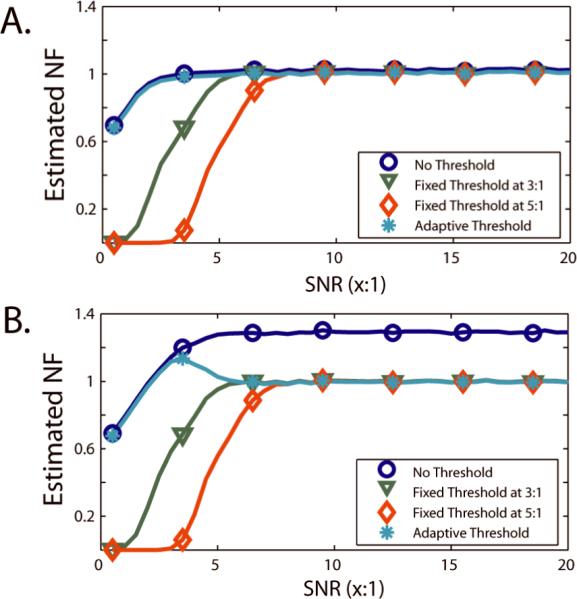
Simulated impact of thresholds on bias in SVNF estimation. 5,000 Monte Carlo iterations were performed for each of 10 Rician distributed observations and for each of 40 linearly spaced SNRs between 1:2 and 20:1. For each dataset, the SVNF was estimated using Eq. (7) with a threshold of 0:1 (no threshold), 3:1, 5:1, and by Eq. (8) (data-adaptive threshold). Second, 5,000 Monte Carlo draws of 1 Rayleigh distributed observation (i.e., an “outlier” with a Rician distribution with SNR=0:1) and 9 Rician distributed observations for each of 40 linearly spaced SNRs between 1:2 and 20:1. For each dataset, the SVNF was estimated using Eq. (7) with a threshold of 0:1 (no threshold), 3:1, 5:1, and by Eq. (8) (data-adaptive threshold). The standard error on all reported estimates is less than 0.005 (for clarity, error bars are not shown).

Case N=2: One Repeated Acquisition

When repeated datasets are available, we form difference images d_i = S_i,1 − S_i,2, between each repeated image pair (for a total of M difference images) and consider regions having high signal intensities. The difference of two i.i.d. Gaussian variables has a zero-mean Gaussian distribution with two-fold increased variance over the original distribution. Thus, the distribution of the resulting set of differences depends only on the SVNF (for locations with sufficient SNR) and not the noise-free mean. In analogy with Eqs. (4) and (7), we form a robust estimator of local standard deviation,

$$\widehat{\sigma }=\frac{1}{\sqrt{2}}{\mathrm{Q}}_{\mathrm{n}}\left(\{\sqrt{{\xi }_1}{d}_1,\sqrt{{\xi }_2}{d}_2,\dots ,\sqrt{{\xi }_M}{d}_M\}\right),$$ (9)

and then use a data adaptive threshold to reduce the image of low SNR,

$${\tilde{\sigma }}_{\mathrm{SRV}2}=\frac{1}{\sqrt{2}}{\mathrm{Q}}_n\left(\sqrt{\xi }\mathbf{d}\backslash \{\sqrt{{\xi }_i}{d}_i:S_i<t\widehat{\sigma }\}\right).$$ (10)

We call this the Spatially Robust Voxel-wise method with 2 repetitions (SRV2) estimator.

Case N≥3: More than One Repeated Acquisition

Finally, when three or more repeated datasets are available, one has redundant measures to estimate the variance for each voxel and each contrast type. To mitigate the impact of artifacts, one can use a robust scale estimator, such as Q_n, to estimate the SVNF for each contrast type,

$${\widehat{\sigma }}_i={\mathrm{Q}}_{\mathrm{n}}\left(\{S_{i,1},S_{i,2},\dots ,S_{i,N}\}\right),$$ (11)

where S_i,j is the signal observation for contrast type i and repetition j. Since the estimator is unbiased when the data are Gaussian distributed, a location estimator (e.g., mean, median) can combine scale estimates (e.g., standard deviation, Q_n) across contrast types. We prefer the use of a robust statistic—in this case the median,

$$\widehat{\sigma }=\text{median}\left(\{{\widehat{\sigma }}_1,{\widehat{\sigma }}_2,\dots ,{\widehat{\sigma }}_i,\dots {\widehat{\sigma }}_M\}\right),$$ (12)

where the ${\widehat{\sigma }}_i$ are estimated for each contrast type with Eq. (10). This estimate is only valid when the data are Gaussian distributed, i.e., when the data are of high SNR. Therefore, in analogy with Eqs. (7) and (10), we estimate the SNR of each contrast type and use a data-adaptive threshold to exclude observations that are of low SNR,

$${\tilde{\sigma }}_{\mathrm{SRVN}}=\text{median}\left(\widehat{\sigma }\backslash \{\widehat{{\sigma }_l}:{\stackrel{‒}{S}}_i<t\widehat{\sigma }\}\right).$$ (13)

We call this the Spatially Robust Voxel-wise method with N repetitions (SRVN) estimator.

Another way to approach this scenario is to examine the set of N repetitions on a pairwise basis and estimate the SVNF with the $\left(\begin{array}{c}\hfill N\hfill \\ \hfill 2\hfill \end{array}\right)$ possible pairings using SRV2. Although not uncorrelated, these estimates are approximately unbiased, so variability can be reduced (without reinforcing bias) by averaging the multiple SVNF estimates,

$${\tilde{\sigma }}_{\mathrm{SRV}2\mathrm{N}}=\text{mean}\left({\left\{{\tilde{\sigma }}_{\mathrm{SRV}2}({\mathbf{s}}_{i_1},{\mathbf{s}}_{i_2})\right\}}_{i_1,i_2\in \left(\begin{array}{c}\hfill N\hfill \\ \hfill 2\hfill \end{array}\right)}\right),$$ (14)

where ${\tilde{\sigma }}_{\mathrm{SRV}2}({\mathbf{s}}_{i_1},{\mathbf{s}}_{i_2})$ denotes the SRV2 SVNF estimate using the i₁th and i₂th images. We call this the SRV2 with N repetitions (SRV2N) estimator.

Regularization of the SVNF

Local estimates of the SVNF may exhibit variations that are inconsistent with the physical knowledge that SVNFs tend to vary smoothly in accordance with coil sensitivity patterns [11]. Such variations can be prominent in regions that are susceptible to artifacts such as motion prone regions and areas that are near to vessels or tissue interfaces. Since variability due to artifacts is not captured in the Rician SVNF model, we suggest a separate method based on robust statistics to mitigate its impact.

To improve robustness against artifacts, we regularize the local SVNF using a coil sensitivity model. We choose a general purpose Chebyshev polynomial regression model with a third degree, two-dimensional polynomial. Chebyshev polynomials are used both for their numeric stability properties and because they have been previously used in modeling coil sensitivity profiles [5,18]. The regularized SVNF $\left(\tilde{\sigma }\right)$ is estimated for all voxels by,

$$\stackrel{\approx }{\sigma }={\mathbf{PW}}^{†}{\left(\mathbf{WP}\right)}^{†}\tilde{\sigma },$$ (15)

where $\tilde{\sigma }$ is a vector of SVNF estimates for each spatial location, P is the matrix of Chebyshev polynomials evaluated at the spatial locations of $\tilde{\sigma }$, W is a weighting matrix, δ indicates the pseudoinverse, and $\underset{\sigma }{\approx }$ is the spatially regularized SVNF estimate. The regularized model can be used to extrapolate SVNF estimate to voxels where there are insufficient local, high SNR observations to estimate $\tilde{\sigma }$.

The weighting matrix, W, should encode the expected variance for the $\tilde{\sigma }$ estimates. The variances of the SVNF estimates in Eqs. (7), (10), and (13) are spatially independent and proportional to the number of observations used during estimation and to the true underlying variance. The covariance of both SDD and SDU SVNF estimates is complicated by spatial correlation due to their use of sliding kernels. For simplicity, we approximate the root-variance matrix, ${\Sigma }^{\frac{1}{2}}$, by a diagonal matrix with entries inversely proportional to the square root of the number of data points used to calculate the local SNR. In the absence of additional modification, ${\Sigma }^{\frac{1}{2}}$ would be the weighting appropriate term, W, to use in the weighted fitting (Eq. (15)). In addition, the signal in low SNR regions is actively and nonlinearly suppressed during reconstruction on many scanners. We compensate for the non-representative SVNF in voxels with low SNR by adapting the weighting matrix as follows,

$${\mathbf{W}}_{i,j}={\Sigma }_{i,j}^{\frac{1}{2}}\left(1-e^{-{\left(\frac{\tilde{\mathrm{s}}}{2\widehat{\sigma }}\right)}^2}\right),$$ (16)

where s̃ is the median signal observed at the voxel and $\widehat{\sigma }$ is the estimated SVNF at the voxel. ${\Sigma }_{i,j}^{\frac{1}{2}}$ is spatially dependent because the thresholding procedures (i.e., Eqs. (6,9,12)) may exclude different sets of observations from each voxel-wise svNF estimate. The equation strongly reduces the weighting for voxels where the approximate SNR is less than 4:1.

The coil sensitivity model (Eq. (15)) is used to regularize each of the SVNF estimators. The regularized SDU and SDD are denoted SDUR and SDDR, respectively. The regularized SRV1, SRV2, and SRVN estimators are called Spatially Robust Regularized methods with 1, 2, N, or “2N” repetitions (SRR1, SRR2, SRRN, SRR2N), respectively.

Experiments

Protocols

We consider SVNF estimation in the context of simulations and empirical studies using two protocols, DTI and T2-relaxometry. Simulation parameters were selected to approximate empirical protocols. Institutional review board approval and written informed consent were obtained prior to all in vivo examinations.

In DTI, the Stejskal-Tanner equation [1] governs the noise-free signal (ν) as a function of reference intensity (S₀),

$$\nu =S_0{e}^{-b{\mathit{g}}^T\mathbf{D}\mathit{g}},$$ (17)

where diffusion weighting is applied along unit direction g with a b-value of b (a control parameter), and D is the local diffusion tensor. Simulations were performed with a FOV of 64×64 voxels with 1 reference and 30 dynamic images corresponding to the Stejskal-Tanner noise-free signal model for a single prolate tensor (λ₁=2 mm²/s, λ₂=λ₃=0.5 mm²/s; fractional anisotropy=0.71) and 30 directions as described by Jones et al. [26] with a b-value of 1000 s/mm². In one empirical study, 15 DTI repeated datasets from a healthy 24 year old male were acquired using a 1.5T MR scanner (Intera, Philips Medical Systems, Best, The Netherlands) with body coil excitation and a six channel phased array sensitivity encoding (SENSE) head-coil for reception. For each dataset, a multi-slice, single-shot EPI (SENSE=2.0), spin echo sequence (TR/TE=2956/100 ms, field-of-view (FOV)=240×240, matrix=96×96, reconstructed to 256×256) was used. Diffusion weighting was applied along 30 distinct directions [26] with a b-factor of 1000 s/mm². Five minimally weighted images (b₀'s) were acquired and averaged in k-space.

In T2-relaxometry, the signaling equation relates the noise-free signal to the NMR parameters T1 and T2 and the sequence parameters TE and TR,

$$\nu =S_0\left(1-2e^{-\frac{TR-TE∕2}{T_1}}+e^{-\frac{TE}{T1}}\right)e^{-\frac{TE}{T2}}\Rightarrow \ln v\approx \ln \mathrm{C}-\frac{TE}{T2}.$$ (18)

When TR≫T1, T1 effects can be neglected and T2 can be estimated directly from observed signal intensities. In our study, 5 repeated datasets from a healthy 29 year old male were acquired using a 1.5T MR scanner (Intera) with body coil excitation and a six channel phased array SENSE head-coil for reception. For each dataset, a single-slice, turbo spin echo (SENSE=2.5) sequence (TR=3000 ms, FOV=220×220, matrix=128×128, reconstructed to 256×256) was acquired. Sixteen echo times (TE) linearly spanning 10 ms to 160 ms were acquired. Due to imperfect RF pulses, odd echoes were contaminated by a stimulated echo component so only the even echoes were used to calculate T2 [14]. Simulations were performed with the same echo times and a true T2 of 80 ms.

Simulation: Voxel-wise SVNF Estimation

To determine the optimal voxel-wise SVNF statistics, GML, SRV2/SRV2N, and SRVN were evaluated with between 2 and 15 repeated DTI and T2 datasets (Figure 2). When 2 or 3 repeated datasets were available, SRV2N estimates were superior to those of GML and SRVN in both applications; thus, we use it for SVNF estimation. When more repeated datasets were available (>6 for DTI or >4 for T2), GML yielded the lowest mean squared error. Therefore, we used GML to estimate a “ground truth” SVNF when no truth model was available, as in the in vivo studies.

Figure 2.

Simulated error rates for voxel-wise estimation. One thousand Monte Carlo iterations were performed for each number of repeated simulated data sets, and the estimated noise variance was compared with the true, simulated noise variance. Datasets were simulated at an SNR of 25:1 based on biophysical models, for DTI (30 directions, single prolate tensor, FA=0.701, Eq. [16]) and T2 relaxometry (16 echoes, T2=80 ms, Eq. [17]). The ordinate is shown with logarithmic scale and arbitrary units.

Simulation: SVNF Estimation

The performance of each of the SVNF estimators (SDU, SDD, SRV1, SRV2/SRV2N) and their regularized counterparts was evaluated in two sets of simulations with DTI and T2 (Figures 3 and 4). The model based approaches (SRV1, SRR1) are positively biased due to both model mismatch and model estimation variability, and result in poor SVNF estimates (Figure 3). Although the voxel-wise SRV2 and SRV2N result in higher MSE than SDD, regularization dramatically improves the MSE (B,D) because these are independent local measures. Solid borders around SDU, SDUR, SDD, and SDDR SVNF estimates indicate regions where no SVNF was estimated due to insufficient kernel overlap. The artifact model increased the MSE for all estimators (compare Figure4A to Figure 3B and Figure4B to Figure 3D). The regularized voxel-wise estimators (SRR2/SRR2N) continued to result in the lowest MSE in the presence of artifacts (Figure 4).

Figure 3.

Simulation of SVNF estimation without artifacts. Regularization increases the MSE of SDU and SDD for both DTI (A,B) and T2 (C,D) simulations. A simulated SVNF (mean SNR=14:1) was constructed using a Chebyshev model such that the center was 81% higher than the periphery. To avoid impacts of spatially varying signal within a contrast type, the described biophysical models were used for all voxels. First, 50 Monte Carlo simulations were performed without artifacts with each of 1 dataset (SDU, SDUR, SRV1, SRR1), 2 datasets (SDD, SDDR, SRV2, SRR2), and 3 datasets (SRV2N, SRR2N). Positive scale bars indicate the standard deviation of the estimates as a percentage of bar height; when no bar is visible, the standard deviation cannot be separately rendered at print resolution.

Figure 4.

Simulation of SVNF estimation with artifacts. 50 Monte Carlo simulations were performed with 2 percent of observations randomly (Bernoulli, p=0.5) attenuated or increased by a factor of 10. Error bars indicate the standard deviation of the estimates as a percentage of bar height.

The local SVNF estimators (SRV1/SRV2/SRV2N) resulted in higher MSE than both methods based on sliding kernels (SDU/SDD). However, once regularized, SRR2 and SRR2N improved MSE by more than a factor of 10 over the kernel estimators in all simulations (DTI and T2 both with and without artifacts). Regularization of SDU and SDD increased MSE.

In vivo: DTI

The 15 DTI datasets were grouped into 15 sets of 1 dataset, 105 sets of 2 datasets and 455 sets of 3 datasets and SVNFs were estimated with each of the methods. For 1 repetition, SDUR and SRR1 result in poor, but nearly equivalent errors. For 2 repetitions, SRV2 and SRR2 both performed better than the SDD methods. Additional improvements in MSE were possible with 3 repetitions over 2 repetitions. Figure 5A shows representative estimates from each of the methods. GML was used to construct a “ground truth” SVNF estimate using all available data (465 images) as shown in the inlay of Figure 5B, and the MSE for each estimation method was calculated over the brain as determined by a manually drawn mask. The SDU method resulted in very large errors due to over estimation of the SVNF near tissue interfaces while the SRV1 method over estimated the SVNF in regions where the model fit was more variable and/or less precise. Compared to SDD, SRV2 improved MSE by 224%, SRR2 by 510%, SRV2N by 449%, and SRR2N by 521%.

Figure 5.

In vivo DTI SVNF Estimation. Panel A shows representative SVNF estimates for each of the estimation methods. These estimates were compared on a voxel-wise basis to the GML estimate constructed using all 15 sessions (Panel B, inset). Panel B plots the MSE within voxels belonging to brain regions.

In Vivo: T2

The 5 T2 datasets were grouped into 5 sets of 1 dataset, 10 sets of 2 datasets, and 10 sets of 3 datasets. The GML estimate with all data showed strong artifacts that are likely due to uncompensated inter-scan motion and pulsatile flow (due to absence of cardiac triggering), so a truth estimate using SRV2N was generated, as shown in Figure 6. When compared with the SVNF estimates using limited data, the model based approach resulted in the lowest error (SRV1). For the methods using repeated datasets, the coil sensitivity model increased error due to propagation from artifact prone regions.

Figure 6.

In vivo T2 SVNF Estimation. The GML SVNF estimate (B) using all data shows strong artifact contributions along the interface between the cortical surface and cerebral spinal fluid. The SRV2N estimate using all data (C) greatly reduces the appearance of artifact contributions, yet a central band of increased SVNF intensity remains, so the SRV2N method was used to construct the ground truth model. The MSE for each set of observations was calculated (D). Regularization did not improve the SDD, SRV2, or SRR2N estimates. Inspection of the individual SVNF estimates (E) reveals artifact contributions in these SVNF that would distort the regularized field.

Discussion

The proposed estimation framework robustly estimates spatially varying SVNFs from in vivo MRI given NFE acquisitions. For convenience, a summary of all the evaluated methods including their key features and observed results is given in Table 1. The use of a data-adaptive threshold achieves minimal loss of power for voxel-wise estimation of noise variance, while remaining robust to observations from non-Gaussian distributions and/or artifacts (Figure 1). Voxel-wise analysis avoids potential correlations or over-dependence on local signal variation, while regularization based on coil sensitivity model provides a physically motivated framework for reducing estimation variability. These fully automated methods are not adversely impacted by spatial correlations, which are common in practice due to up-sampling and interpolation.

Within the family of proposed estimators, simulations demonstrate that the appropriate local estimator depends on the problem domain and the sample size. For small sample sizes, our method compares favorably to strict maximum likelihood methods even without artifact (Figure 2). When the coil model is appropriate, SVNF estimates may be obtained with two or more repeated datasets, which offer dramatic improvements over SDD (Figure 3 and Figure 4). In typical research studies a scan may be repeated a few (N=2–5) times, and simulations indicate that SRV2N achieved the lowest MSE. However, simulations suggest that GML and SRVN could achieve lower MSE when many repeated observations (N>5) are available, so for SVNF analysis given many repeated acquisitions it might be preferable to use SRVN or a robust adaptation of GML. The accuracy and precision of each SVNF estimation method depends on the underlying signal characteristics and SVNF process, so it is sensible to assess the signal-to-noise characteristics and prevalence of artifact to ensure an appropriate choice of local estimator and coil sensitivity model. These aspects would be interesting areas for future study.

When one dataset is available, SVNF estimation is either confounded by model mismatch (SRV1/SRR1) or spatial signal variability (SDU/SDUR). In simulations with a uniform truth model, the SDU leads to superior results. These findings remain robust in the presence of simulated artifacts. Empirically, tensor model leave-one-out residuals (SRV1) do not lead to accurate SVNF estimates, while the T2 model leave-one-out residuals (SRV1) lead to best results due to insensitivity to inter-scan motion or pulsatile flow. Diffusion tensors are known to be a loose approximation of the true three-dimensional diffusivity function, so it is natural to expect that there would be substantial variability due to the model in the leave-one-out residual estimates and the SRV1 SVNF estimates would be of high MSE (Figure 5). The T2 model, on the other hand, makes more minimal approximations and leads to much stronger correlations between the model fit, so the SRV1 leave-one-out estimates are more precise. In fact, the T2 SRV1/SRR1 estimates are of the lowest MSE due to their reduced sensitivity to inter-scan motion (Figure 6). These results suggest opportunities for using minimally biased model estimation methods, which would be an interesting area for future investigation. For example, the svNF could be iteratively estimated in conjunction with noise-aware modeling methods and could lead to reduced residual bias and improved svNF estimation.

The empirical studies demonstrate that coil sensitivity model and dominance of artifacts play important roles in SVNF estimation. In the DTI study, the coil sensitivity model dramatically improves SVNF estimation (Figure 5). In the T2, there appears to be a substantial influence of bulk motion and inflow artifacts on the estimated SVNFs, so the coil model regularization does not improve the SVNF estimates for N>2 (Figure 6). For both the DTI and T2 studies, the SDU SVNF estimates are quite inaccurate since the noise-free signals are not uniform in intensity over local regions, and the SDD method is affected by the substantial correlation between adjacent voxels. The DTI studies were multislice sequences and signal changes due motion could be readily compensated, and all estimated SVNFs showed strong spatial dependence which is in visual accord with the proposed coil sensitivity model. The T2 studies involved a single-slice acquisition which is sensitive to inflow effects and out of plane motion, while the impact of coil sensitivity was decreased through a TSE readout as opposed to an EPI readout. Interesting, the inflow effects were not readily visible on the image data, but were instantly apparent on the robust SVNF estimate, which hints at applications for SVNF estimation in artifact detection and image quality assessment.

In conclusion, the proposed analysis of NFE acquisitions lead to robust and accurate characterizations of SVNFs with data that are routinely available in clinical and research. Within the proposed class, there are numerous feasible estimators given the choice of robust statistics (e.g., median versus Q_n) or interchange of space, scale estimation, or model residuals (e.g., GML, SRV1, SRV2, SRVN, SRV2N). Within the set of evaluated methods, we see that there can be substantial gain from using repeated acquisitions, but the improvement is moderate after the first pair. The selected robust statistics presented herein are based on our best judgments. However, it is impossible to exhaustively evaluate all heuristic design choices of robust estimators within the proposed family since there are unlimited design possibilities to achieve different tradeoffs between outlier insensitivity and optimality when assumptions are met. It will certainly be interesting and worthwhile to explore variants of these design choices (e.g., which scale and location estimators, outlier rejection/thresholding procedure, etc.). The most appropriate choice of estimators will depend on the context of specific applications and will be further investigated in future studies.

References

- 1.Basser PJ, Jones DK. Diffusion-tensor MRI: theory, experimental design and data analysis - a technical review. NMR Biomed. 2002;15(7–8):456–467. doi: 10.1002/nbm.783. [DOI] [PubMed] [Google Scholar]
- 2.Brummer ME, Mersereau RM, Eisner RL, Lewine RRJ. Automatic detection of brain contours in MRI data sets. IEEE Trans Med Imaging. 1993;12(2):153–166. doi: 10.1109/42.232244. [DOI] [PubMed] [Google Scholar]
- 3.Bryant RG. The dynamics of water-protein interactions. Annu Rev Biophys Biomol Struct. 1996;25:29–53. doi: 10.1146/annurev.bb.25.060196.000333. [DOI] [PubMed] [Google Scholar]
- 4.Covel MM, Hearshen DO, Carson PL, Chenevert TL, Shreve P, Aisen AM, Bookstein E, Murphy BW, Martel W. Automated analysis of multiple performance characteristics in MRI systems. Med Phys. 1986;13(6):815–823. doi: 10.1118/1.595804. [DOI] [PubMed] [Google Scholar]
- 5.Davis PJ. Interpolation and Approximation: Dover. 1975. [Google Scholar]
- 6.De Wilde JP, Lunt JA, Straughan K. Information in magnetic resonance images: evaluation of signal, noise, and contrast. Med Biol Eng Comput. 1997;35:259–265. doi: 10.1007/BF02530047. [DOI] [PubMed] [Google Scholar]
- 7.Firbank MJ, Coulthard A, Harrison RM, Williams ED. A comparison of two methods for measuring the signal to noise ratio on MR images. Phys Med Biol. 1999;44:N261–N264. doi: 10.1088/0031-9155/44/12/403. [DOI] [PubMed] [Google Scholar]
- 8.Gudbjartsson H, Patz S. The Rician distribution of noisy MRI data. Magn Reson Med. 1995;34(6):910–914. doi: 10.1002/mrm.1910340618. [DOI] [PMC free article] [PubMed] [Google Scholar]
- 9.Haacke EM, Brown RW, Thompson MR, Venkatesan R. Magnetic Resonance Imaging: Physical Principles and Sequence Design. Wiley-Liss; New York: 1999. [Google Scholar]
- 10.Henkelman RM. Measurement of signal intensities in the presence of noise in MR images. Med Phys. 1985;12(2):232–233. doi: 10.1118/1.595711. [DOI] [PubMed] [Google Scholar]
- 11.Jones DK, Basser PJ. “Squashing peanuts and smashing pumpkins”: how noise distorts diffusion-weighted MR data. Magn Reson Med. 2004;52(5):979–993. doi: 10.1002/mrm.20283. [DOI] [PubMed] [Google Scholar]
- 12.Kaufman L, Kramer DM, Crooks LE, Ortendahl DA. Measuring signal-to-noise ratios in MR imaging. Radiology. 1989;173:265–267. doi: 10.1148/radiology.173.1.2781018. [DOI] [PubMed] [Google Scholar]
- 13.Kellman P, McVeigh ER. Image Reconstruction in SNR Units: A General Method fo SNR Measurement. Magn Reson Med. 2005;54:1439–1447. doi: 10.1002/mrm.20713. [DOI] [PMC free article] [PubMed] [Google Scholar]
- 14.Majumdar S, Orphanoudakis SC, Gmitro A, O'Donnell M, Gore JC. Errors in the measurements of T2 using multiple-echo MRI techniques. I. Effects of radiofrequency pulse imperfections. Magn Reson Med. 1986;3(3):397–417. doi: 10.1002/mrm.1910030305. [DOI] [PubMed] [Google Scholar]
- 15.McGibney G, Smith MR. An unbiased signal-to-noise ratio measure for magnetic resonance images. Med Phys. 1993;20(4):1077–1078. doi: 10.1118/1.597004. [DOI] [PubMed] [Google Scholar]
- 16.Murphy BW, Carson PL, Ellis JH, Zhang YT, Hyde RJ, Chenevert TL. Signal-to-noise measures for magnetic resonance imagers. Magn Reson Med. 1993;11:425–428. doi: 10.1016/0730-725x(93)90076-p. [DOI] [PubMed] [Google Scholar]
- 17.Parker DL, Gullberg GT. Signal-to-noise efficiency in magnetic resonance imaging. Med Phys. 1990;17(2):250–257. doi: 10.1118/1.596503. [DOI] [PubMed] [Google Scholar]
- 18.Pham DL, Bazin P-L. Simultaneous Boundary and Partial Volume Estimation in Medical Images. Lecture Notes in Computer Science (Medical Image Computing and Computer-Assisted Intervention) 2004:119–126. [Google Scholar]
- 19.Pruessmann KP, Weiger M, Scheidegger MB, Boesiger P. SENSE: sensitivity encoding for fast MRI. Magn Reson Med. 1999;42(5):952–962. [PubMed] [Google Scholar]
- 20.R. M. Henkelman GJSSJG Magnetization transfer in MRI: a review. NMR in Biomedicine. 2001;14(2):57–64. doi: 10.1002/nbm.683. [DOI] [PubMed] [Google Scholar]
- 21.Ramsey NF, Hoogduin H, Jansma JM. Functional MRI experiments: acquisition, analysis and interpretation of data. European Neuropsychopharmacology. 2002;12(6):517–526. doi: 10.1016/s0924-977x(02)00101-3. [DOI] [PubMed] [Google Scholar]
- 22.Rousseeuw PJ, Croux C. Alternatives to the Median Absolute Deviation. J Am Stat Assoc. 1993;88(424):1273–1283. [Google Scholar]
- 23.Sijbers J, den Dekker AJ, Van Audekerke J, Verhoye M, Van Dyck D. Estimation of the noise in magnitude MR images. Magn Reson Imag. 1998;16(1):87–90. doi: 10.1016/s0730-725x(97)00199-9. [DOI] [PubMed] [Google Scholar]
- 24.Sijbers J, den Dekker AJ. Maximum likelihood estimation of signal amplitude and noise variance from MR data. Magn Reson Med. 2004;51(3):586–594. doi: 10.1002/mrm.10728. [DOI] [PubMed] [Google Scholar]
- 25.Sijbers J, Poot D, den Dekker AJ, Pintjens W. Automatic estimation of the noise variance from the histogram of a magnetic resonance image. Phys Med Biol. 2007;52(5):1335–1348. doi: 10.1088/0031-9155/52/5/009. [DOI] [PubMed] [Google Scholar]
- 26.Skare S, Hedehus M, Moseley ME, Li TQ. Condition number as a measure of noise performance of diffusion tensor data acquisition schemes with MRI. J Magn Reson. 2000;147(2):340–352. doi: 10.1006/jmre.2000.2209. [DOI] [PubMed] [Google Scholar]
- 27.Wood JC, Johnson KM. Wavelet packet denoising of magnetic resonance images: importance of Rician noise at low SNR. Magn Reson Med. 1999;41(3):631–635. doi: 10.1002/(sici)1522-2594(199903)41:3<631::aid-mrm29>3.0.co;2-q. [DOI] [PubMed] [Google Scholar]
- 28.Yihong Y. Perfusion MR imaging with pulsed arterial spin-labeling: Basic principles and applications in functional brain imaging. Concepts in Magnetic Resonance. 2002;14(5):347–357. [Google Scholar]