A general-purpose baseline estimation algorithm for spectroscopic data

Abstract

A common feature of many modern technologies used in proteomics—including nuclear magnetic resonance imaging and mass spectrometry—is the generation of large amounts of data for each subject in an experiment. Extracting the signal from the background noise, however, poses significant challenges. One important part of signal extraction is the correct identification of the baseline level of the data. In this article, we propose a new algorithm (the “BXR algorithm”) for baseline estimation that can be directly applied to different types of spectroscopic data, but also can be specifically tailored to different technologies. We then show how to adapt the algorithm to a particular technology—matrix-assisted laser desorption/ionization Fourier transform ion cyclotron resonance mass spectrometry—which is rapidly gaining popularity as an analytic tool in proteomics. Finally, we compare the performance of our algorithm to that of existing algorithms for baseline estimation.

The BXR algorithm is computationally efficient, robust to the type of one-sided signal that occurs in many modern applications (including NMR and mass spectrometry), and improves on existing baseline-estimation algorithms. It is implemented as the function baseline in the R package FTICRMS, available either from the Comprehensive R Archive Network (http://www.r-project.org/) or from the first author.

1 Introduction

A common feature of many modern technologies used in proteomics—including nuclear magnetic resonance imaging and mass spectrometry—is the generation of large amounts of data for each subject in an experiment. Extracting the signal from the background noise, however, poses significant challenges. One important part of signal extraction is the correct identification of the baseline level of the data. In this article, we first generalize an algorithm of Xi and Rocke [1] which was developed for NMR baseline correction and show how it can be applied to data from generic spectroscopic technologies. We also indicate how it can be adapted to the unique qualities of different technologies and illustrate this by adapting it to a specific technology: matrix-assisted laser desorption/ionization Fourier transform ion cyclotron resonance mass spectrometry (MALDI FT-ICR MS). Finally, we compare the performance of our algorithm to that of existing algorithms for baseline estimation.

2 Methods

2.1 What is a baseline?

There are different possible interpretations of what exactly a “baseline” is in spectroscopic analysis. If it is assumed that the signal is all positive standing out from a (theoretically) zero baseline level, then some kind of (smoothed) running minimum would be an appropriate baseline. This is the approach taken in software packages such as Cromwell [2], LCMS-2D [3], LIMPIC [4], PrepMS [5], and PROcess [6]. Alternatively, if the noise is assumed to fluctuate about a baseline level (like in an independent, identically-distributed (iid) normal case), then some measure of center (median, mean, etc.) is more appropriate. This is the approach taken in software packages such as msInspect [7]. Software packages such as LMS [8] have options to compute either of these types of baselines. (A third common type of analysis is continuous wavelet analysis, which does not have a separate baseline correction step as such; the baseline is automatically removed as part of the wavelet transformation. This is the approach taken in software packages such as MassSpecWavelet [9] and OpenMS [10].)

The Xi-Rocke algorithm uses the second interpretation of baseline (measure of center of the noise), and as explained in Section 3, this is the appropriate way to analyze (in particular) MALDI FT-ICR MS spectra, and is arguably appropriate in other applications. In the remainder of this article we will concentrate on this type of baseline and compare our algorithm to LMS. (msInspect was designed for liquid chromatography mass spectrometry and is not directly comparable to our current algorithm.)

2.2 The BXR algorithm

Suppose that the data have the form (x_t, y_t) for t = 1, …, n. Xi and Rocke [1] proposed using the score function in Equation (1) to estimate the baseline for NMR data.

$$F(\{b_t\})=\sum _{t=1}^n{b}_t-A_1\sum _{t=2}^{n-1}{(b_{t-1}-2b_t+b_{t+1})}^2-A_2\sum _{t=1}^n{[{(b_t-y_t)}_{+}]}^2$$ (1)

Here, z₊ ≡ max{z, 0}, b_t represents the value of the baseline at the t-th data point, and A₁ and A₂ are positive constants to be determined. We maximize this score function over all possible values of {b_t} to find the baseline¹. The first term in F represents the overall height of the baseline. The last term is negative only when the baseline is above the data points, so it penalizes baseline values that lie too far above the data and helps ensure that the estimated baseline will go through the middle of the data. The middle term is a measure of the curvature of the baseline, so maximizing F will prevent the estimated baseline from curving too sharply.

To make the analysis easier, we change notation. Let b = (b₁, …, b_n)′—where the prime symbol represents the transpose of a vector or matrix—be a column vector containing the values of the baseline, and similarly let y = (y₁, …, y_n)′ contain the measured values of the spectrum. Let (S) be the indicator function for the set S and let 1 be an n × 1 column vector of ones. Finally, it will be useful to allow A₁ and A₂ to vary with t, taking values ${\{A_{1,t}\}}_{t=2}^{n-1}$ and ${\{A_{2,t}\}}_{t=1}^n$, respectively. We can then rewrite Equation (1) in vector/matrix notation as

$$F(\mathit{b})={\mathbf{1}}^{\prime }\mathit{b}-{\mathit{b}}^{\prime }{\mathbf{\Delta }}_2\mathit{b}-(\mathit{b}-{\mathit{y}}^{\prime })\mathit{N}(\mathit{b}-\mathit{y}),$$ (2)

where N is an n × n diagonal matrix with entries A_2,t (b_t > y_t), and ${\mathbf{\Delta }}_2={\mathit{M}}_2^{\prime }{\mathit{A}}_1{\mathit{M}}_2$, where

$${\mathit{M}}_2=\left[\begin{array}{ccccccc}1& -2& 1& 0& 0& 0& \\ 0& 1& -2& 1& 0& 0& \cdots \\ 0& 0& 1& -2& 1& 0& \\ & & ⋮& & & & \ddots \end{array}\right]$$

is an (n−2) ×n matrix and A₁ is an (n − 2) × (n − 2) diagonal matrix with entries A_1,t. We will refer to the process of maximizing this modified score function with respect to the baseline b as the Barkauskas-Xi-Rocke (BXR) algorithm.

Note that the only change that the BXR algorithm makes over Xi and Rocke’s original algorithm is allowing A₁ and A₂ to vary with t. This seemingly minor change has a profound impact on the effectiveness of the algorithm in the analysis of real-world data, however, as we show in Sections 2.3 and 3.

To maximize the function in Equation (2), we calculate the gradient and Hessian:

$$\begin{array}{l}\nabla F(\mathit{b})=\mathbf{1}-2{\mathbf{\Delta }}_2\mathit{b}-2\mathit{N}(\mathit{b}-\mathit{y})\\ [H(F)](\mathit{b})=-2({\mathbf{\Delta }}_2+\mathit{N}).\end{array}$$

Note that ∇F is continuous everywhere, and H(F) is continuous except for jump discontinuities where b_t = y_t for some t. Also, Δ₂ and N are both positive semidefinite (because b′Δ₂b is a sum of squares, and N is diagonal with nonnegative entries). Thus, Δ₂ + N is positive semidefinite and will be positive definite unless Δ₂ and N have a common null vector. But from the form ${\mathbf{\Delta }}_2={\mathit{M}}_2^{\prime }{\mathit{A}}_1{\mathit{M}}_2=({\mathit{A}}_1^{1/2}{\mathit{M}}_2{)}^{\prime }{\mathit{A}}_1^{1/2}{\mathit{M}}_2$, we see that $\text{rank}({\mathbf{\Delta }}_2)=\text{rank}({\mathit{A}}_1^{1/2}{\mathit{M}}_2)=n-2$, and that x′Δ₂x = 0 exactly when x is a linear combination of 1 and n ≡ (1, …, n)′. Furthermore, the only way that x′Nx = 0 is if x_t = 0 whenever b_t > y_t. But a nontrivial linear combination of 1 and n can have at most one zero entry, so in order for the two matrices to have a common null vector, the baseline would have to be below all but at most one point of the data. This will clearly not happen in any reasonable data set, so we see that H(F) is −2 times the sum of two positive semidefinite matrices that have no common nullspace near any potential maximum. Thus, we see that in any reasonable data set there will be a unique maximum, since H(F) is negative semidefinite overall and negative definite near any (reasonable) potential maximum. We can thus find the maximum by using Newton’s method using a reasonable starting point (e.g., median(y) · 1), and the BXR algorithm is virtually guaranteed to converge to the global maximum. (Technically, in most applications it will be a quasi-Newton’s method, since the matrices Δ₂ and N will depend non-trivially on b—the quantity we are trying to estimate—and at each iteration we will be using the currently-estimated baseline to approximate b. Thus, at each step we will only be approximating the gradient and Hessian.)

2.3 Calculating A_1,t and A_2,t

Since the estimated baseline should be linear in the data (i.e., for any constants m and c, if b corresponds to y, then mb + c should correspond to my + c) and should be invariant under sampling more or fewer points in the spectrum, Xi and Rocke argue that in their original algorithm, A₁ should have the form $A_1=n^4{A}_1^{\ast }/\sigma$, where σ is a normalizing constant based on y. (Xi and Rocke use an estimate of the noise standard deviation; hence the use of σ to denote the constant.) In this article, we will allow the normalizing constant σ to vary with t as σ_t but leave the smoothing parameter $A_1^{\ast }$ constant, giving us the form $A_{1,t}=n^4{A}_1^{\ast }/{\sigma }_t$. To decide on a reasonable value of $A_1^{\ast }$, we use a result from Barkauskas et al. [12] that the autocorrelation function (ACF) of a (non-stationary) time series with {(Y_t+k − Y_t+k)(Y_t − Y_t)} ≈ 0 for sufficiently large k eventually oscillates around a value that is approximately equal to

$$\frac{\text{Var}(\mathit{b})}{\text{Var}(\mathit{y})}.$$ (3)

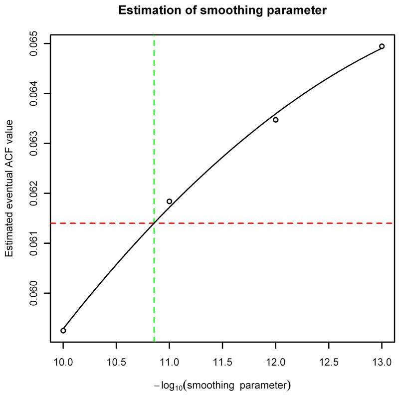
The optimal value of $A_1^{\ast }$ can then be estimated by calculating the baseline b using different choices for $A_1^{\ast }$ and seeing which one gives the best match to the ACF of the noise portion of the spectrum when substituted into Equation (3). (See Figure 3 in Section 3 for an example of this applied to a MALDI FT-ICR spectrum.)

Figure 3.

Value of Var(b)/Var(y) for baselines estimated from the noise spectrum in Figure 2 using various choices of smoothing parameter $A_1^{\ast }$. The solid line is the least-squares fit parabola for the data points, and the horizontal dashed line is the eventual value of the ACF of the spectrum.

In order to determine A_2,t, we set the t-th coordinate of ∇F equal to zero and assume that the baseline is flat, so that the middle term drops out. Let Y_t be the underlying random variable whose realization is given by y_t. We want to choose A_2,t so that the function is maximized at b_t = g(Y_t) for some function g. Thus, we want

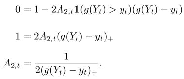(Of course, if g(Y_t) were known, there would be no need to run the algorithm.) One obvious choice for g(Y_t) is the expected value Y_t. For this choice of g(Y_t) in the case that the data are assumed to be iid normal with variance σ², then we might choose

$$A_{2,t}=\frac{1}{2\mathbb{E}\{{(\mathbb{E}{Y}_t-Y_t)}_{+}\}}=\frac{1}{2(\sigma /\sqrt{2\pi })}=\frac{\sqrt{\pi /2}}{\sigma },$$

which recovers the result in Xi and Rocke [1].

We observe that for an arbitrary random variable Y, we have {(Y − Y)₊} = |Y − Y|/2. Thus, if there is no information about the distribution of the random variables {Y_t}, then a reasonable choice might be A_2,t = (b̂_t > y_t)/(b̂_t − y_t), where b̂_t is the current estimate of the baseline (i.e., the current estimate of Y_t).

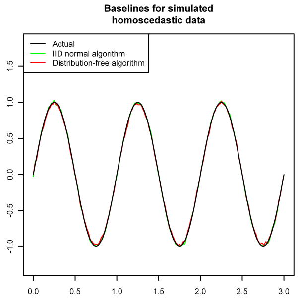
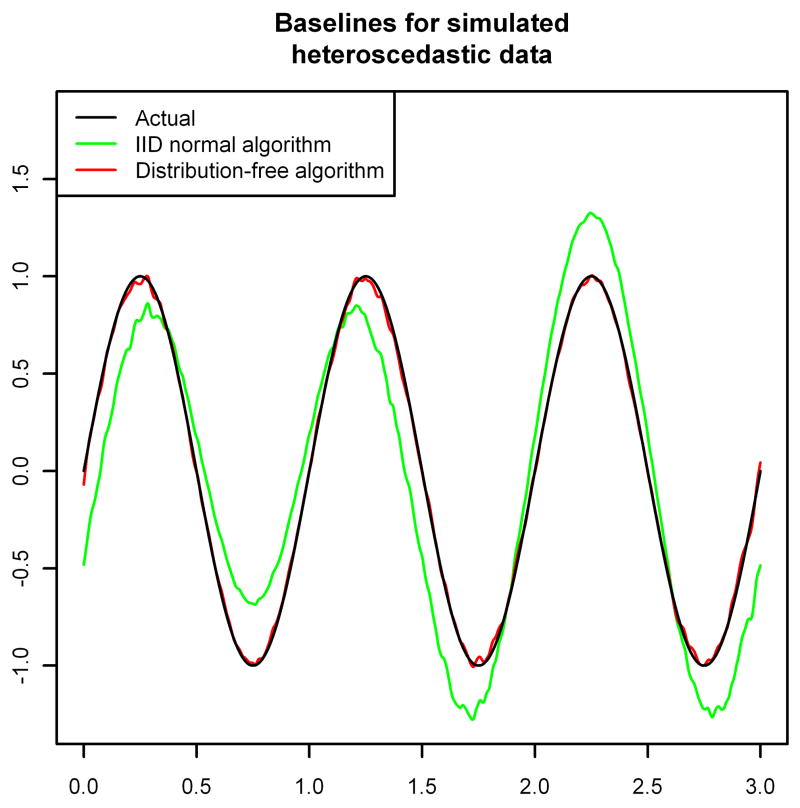
Figure 1 shows the effect of these choices on the estimated baseline. We ran two simulations of 973,720 observations (the number of observations in the “noise” spectrum analyzed in Section 3), each with x-coordinates equally spaced between zero and three and with baseline given by y = sin(2πx). In the first simulation we used iid (0, 1) noise added to the baseline, and in the second we used independent $\mathcal{N}(0,{\sigma }_x^2)$ noise, where σ_x = 1 + 0.5 cos(4πx/3). We used $A_1^{\ast }={10}^{-11}$ and a constant value for σ_t estimated by dividing the spectrum into 1024 (roughly) equal-sized sets of points, calculating the standard deviation of each set of points, then finding the average standard deviation using the estimate of center from Tukey’s biweight with K = 9. We ran the BXR algorithm twice on each set of simulated data, once with each choice of A_2,t above.

Figure 1.

Baseline estimation for simulated homoscedastic and heteroscedastic normal data using each of the two possible choices for A_2,t from Section 2.3.

For the data generated with homoscedastic noise, both versions of the BXR algorithm perform well, with only a small amount of bias near the extreme values of the baseline (Figure 1, top). The major advantage here is that the algorithm that assumes homoscedasticity runs much faster (using roughly 10–20% of the computing time, depending on the exact convergence criterion chosen). However, if the noise is actually heteroscedastic, then assuming homoscedasticity causes the BXR algorithm to badly mis-estimate the baseline—underestimating the baseline when the variance is above average and overestimating the baseline when the variance is below average (Figure 1, bottom). The distribution-free version of the BXR algorithm, however, still produces a result that is almost indistinguishable from the true baseline. Thus, if the noise can reasonably be assumed to be iid normal, then $A_{2,t}={\sigma }^{-1}\sqrt{\pi /2}$ is a good choice, but if the noise is heteroscedastic with unknown distribution, then A_2,t = (b̂_t > y_t)/(b̂_t − y_t)—where b̂_t is the current estimate of the baseline—should be preferred.

Of course, if information on the distribution of the noise for a particular technology is available, it would be advantageous to explore whether distribution-specific choices for A_1,t and A_2,t would work better than the distribution-free choices. In the next section, we will show how to do this for the particular case of MALDI FT-ICR MS data.

3 Application to MALDI FT-ICR MS data

Matrix-assisted laser desorption/ionization Fourier transform ion cyclotron resonance mass spectrometry (MALDI FT-ICR MS) is a technique for high mass-resolution analysis of substances that is rapidly gaining popularity as an analytic tool in proteomics. Typically in MALDI FT-ICR MS, a sample (the analyte) is mixed with a chemical that absorbs light at the wavelength of the laser (the matrix) in a solution of organic solvent and water. The resulting solution is then spotted on a MALDI plate and the solvent is allowed to evaporate, leaving behind the matrix and the analyte. A laser is fired at the MALDI plate and is absorbed by the matrix. The matrix breaks apart and transfers a charge to the analyte, creating the ions of interest (with fewer fragments than would be created by direct ablation of the analyte with a laser). The ions are guided with a quadrupole ion guide into the ICR cell where the ions cyclotron in a magnetic field. While in the cell, the ions are excited and ion cyclotron frequencies are measured. The angular velocity, and therefore the frequency, of a charged particle is determined solely by its mass-to-charge ratio. Using Fourier analysis, the frequencies can be resolved into a sum of pure sinusoidal curves with given frequencies and amplitudes. The frequencies correspond to the mass-to-charge ratios and the amplitudes correspond to the concentrations of the compounds in the analyte. FT-ICR MS is known for high mass resolution, with separation thresholds on the order of 10⁻³ Daltons (Da) or better [13, 14].

As an application of the methods developed in Section 2, we use them on two MALDI FT-ICR spectra, one of which is a “noise” spectrum—one created with no analyte or matrix, pictured in Figure 2—and the other of which was prepared for a cancer study [15] with human blood serum as the analyte. The spectra analyzed in this article were recorded in the Lebrilla lab in the Chemistry Department at the University of California at Davis on an external source MALDI FT-ICR instrument (HiResMALDI, IonSpec Corporation, Irvine, CA) equipped with a 7.0 T superconducting magnet and a pulsed Nd:YAG laser 355 nm. The serum sample was collected at the University of California at Davis Cancer Center; the patient gave written informed consent under an IRB-approved protocol.

Figure 2.

A typical noise spectrum. The spike extending off the top of the picture is actually two peaks at frequencies of 41.21 kHz and 42.21 kHz which extend upward to intensities of approximately 222.7 and 95.4, respectively.

The BXR algorithm is especially suited to analyzing MALDI FT-ICR spectra because of the following property, first observed in Barkauskas et al. [12]: the data obtained by dividing the noise portion of a MALDI FT-ICR spectrum by the expected value at each point can be closely modeled by a causal and invertible autoregressive, moving-average time series with generalized gamma innovations. Thus, identifying the mean level of the noise determines the entire distribution of the noise, which leads to a nice method for identifying peaks in a MALDI FT-ICR spectrum as either noise or signal.

It follows that if we consider the random variables $Y_t^{\prime }=Y_t/\mathbb{E}{Y}_t$, then { $Y_t^{\prime }$} should be identically distributed with mean 1. (Note that { $Y_t^{\prime }$} are not independent; the autocorrelation function is non-trivial.) Thus, we get

$$\mathbb{E}\{{(\mathbb{E}{Y}_t-Y_t)}_{+}\}=\mathbb{E}{Y}_t·\mathbb{E}\{{(1-Y_t^{\prime })}_{+}\}.$$

Using the spectrum in Figure 2 as {Y_t} (and running means to estimate {Y_t}) gives us $\mathbb{E}\{{(1-Y_t^{\prime })}_{+}\}=0.2100706$. For each iteration we can use the currently estimated value of the baseline b̂_t as an estimate for Y_t, so we see that for this spectrum we should use A_2,t = 1/0.4201412b̂_t. Similarly, to obtain an appropriate value of σ_t, we observe that since the standard deviation of $Y_t^{\prime }$ estimated from the spectrum is 0.522659, we can use σ_t = 0.522659b̂_t.

To choose an appropriate value of $A_1^{\ast }$, we tried values of 10^−j for j = 10, …, 13 and found that the value of Var(b)= Var(y) was closest to the eventual value of the ACF of the noise spectrum when $-{log}_{10}{A}_1^{\ast }\approx 10.855$ (see Figure 3).

For each of the two spectra, we calculated the baseline using four methods: a running Tukey’s biweight with K = 9 and bandwidth 8001; and the BXR algorithm with $A_1^{\ast }={10}^{-10.855}$ and A_2,t chosen to be one of the three choices ${\sigma }^{-1}\sqrt{\pi /2}$ (the “iid normal method”, which is just Xi and Rocke’s original algorithm), or (b̂_t > y_t)/(b̂_t − y_t) (the “distribution-free method”), or 1/0.4201412b̂_t (the “distribution-specific method”), where b̂_t is the current estimate of the baseline at point t. For the first two choices of A_2,t we used σ_t calculated in the same way as for the simulated data in Section 2.3; for the last choice of A_2,t, we used σ_t = 0.522659b̂_t. We then computed the ratio of each of the estimated baselines to a running means estimate.

For the noise spectrum, we used running means with bandwidth 8001. The noise spectrum has two spikes at frequencies of 41.21 kHz and 42.21 kHz which extend upward to intensities of approximately 222.7 and 95.4, respectively, and are apparently instrumental noise (they have no isotope peaks; if they were real compounds, the isotope peaks should be easily large enough to show above the noise). In the calculation of the running means, we set the values of the spectrum at frequencies corresponding to these two peaks to be missing.

For the serum spectrum, the presence of multiple large peaks would badly skew the running means. To get a reasonable estimate of the running means of the noise portion of the spectrum, we used a baseline calculated using the BXR algorithm with parameters A_1,t and A_2,t as for the noise spectrum and set the values of the spectrum at frequencies corresponding to any peak that reaches at least 3.7996 times higher than that to be missing. (From simulations of noise spectra, this is approximately equivalent to taking 4.5 standard deviations above the mean for iid normal data.) We then used running means with bandwidth 8001.

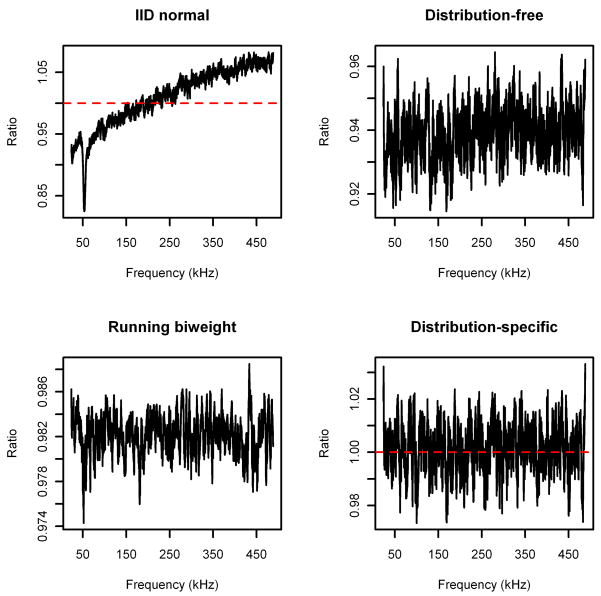
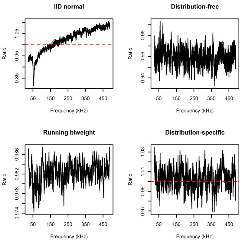
The results for the noise spectrum are displayed in Figure 4, and the results for the serum spectrum are displayed in Figure 5. Note that each algorithm performs similarly for both spectra. Specifically, the iid normal method underestimates the baseline for small frequencies (where the noise variance is large) and overestimates the baseline for large frequencies (where the noise variance is small), as expected. The distribution-free method does much better, but is still consistently underestimating the baseline. Furthermore, in the noise spectrum the bias increases in absolute value as the frequency decreases. The running Tukey’s biweight underestimates the running means by a fairly consistent amount (although by less than the distribution-free method), which is not surprising, since a simple calculation shows that the distribution of the noise is right-skewed. Finally, we see that the baseline estimated using the distribution-specific parameters is (on average) unbiased.

Figure 4.

Ratio of estimated baselines over running means (bandwidth 8001) for noise spectrum.

Figure 5.

Ratio of estimated baselines over running means (bandwidth 8001) for serum spectrum.

Thus, applying the distribution-specific BXR algorithm to a MALDI FT-ICR spectrum is roughly equivalent to simply calculating running means for the noise portion of that spectrum. However, the BXR algorithm has two main advantages over running means. The first is speed: the BXR algorithm uses roughly half the computing time of the running means. (Of course, optimizing each algorithm could change this. Also, as noted in Yang et al. [16], even aside from issues of algorithm optimization, running times are only really comparable for programs in the same language. Thus, comparing run times of various algorithms should only be considered as a rough guideline.) More importantly, the negativity penalty A_2,t in the BXR algorithm only comes into play when the baseline is above the data. If the data is above the baseline, it doesn’t matter by how much. Thus, the extremely large values in a spectrum which constitute the signal are automatically ignored by the BXR algorithm, while extra work is needed to ignore the signal when calculating the running means (as we had to do above in the estimation of the running means for the serum spectrum).

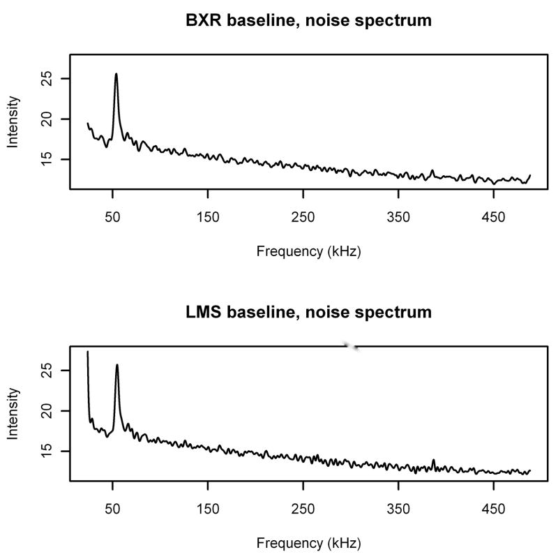
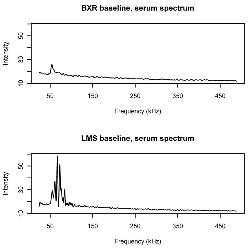
This is even more clearly illustrated by a comparison of baselines computed by the BXR algorithm and the LMS algorithm (Figures 6 and 7). Note that for the noise spectrum, the two baselines are extremely close to each other, except for an apparent edge effect at low frequencies for the LMS algorithm. In fact, except near the peak and at the low frequency edge, the estimates never differ by more than ±5%. However, in the areas of the serum spectrum that have signal, the estimate from the LMS algorithm is pulled up toward the signal drastically, reaching up to more than three times as high as the BXR estimate. In the areas with little or no signal (frequencies greater than 100 kHz), the LMS and BXR estimates are still within ±5% of each other. While there is a mild inflation of the baseline in the presence of signal in the BXR algorithm, it is only inflated up to 13% larger than the estimated baseline for the noise spectrum. Thus, it is clear that the BXR algorithm is far less sensitive to the presence of signal than the LMS algorithm.

Figure 6.

Estimated baselines for noise spectrum calculated using BXR (top) and LMS (bottom) algorithms.

Figure 7.

Estimated baselines for serum spectrum calculated using BXR (top) and LMS (bottom) algorithms.

4 Future Directions

One obvious question is how many of this results in this article are due to the particular experimental setup used to generate the spectra analyzed in this article and how much can be generalized. One encouraging sign is that the coefficients obtained in Section 3 are consistent in replicates; for a set of 56 noise spectra similar to the one displayed in Figure 2, the estimated values of $\mathbb{E}\{{(1-Y_t^{\prime })}_{+}\}$ had a mean of 0.210011 and a standard deviation of 2.46 × 10⁻⁴, while the estimated values for the standard deviation of $Y_t^{\prime }$ had a mean of 0.522584 and a standard deviation of 6.36 × 10⁻⁴. Thus, it would seem to be justified to use the mean values of the two parameters for analyses on any spectrum generated on the same MALDI FT-ICR machine rather than having to calculate them individually for each spectrum. Whether or not these same numbers would apply to other MALDI FT-ICR machines is unknown, but it seems likely that at the very worst, each experimenter could use the techniques described in this article to determine the appropriate numbers for his or her experimental setup and use those.

Additionally, we have concentrated on the case the the estimated quantity is Y_t because that is the key quantity in MALDI FT-ICR MS. However, any measure of center g(Y_t) which is homogeneous of degree 1 (i.e., g(cY_t) = c · g(Y_t)) can be used instead. For example, replacing g(Y_t) = Y_t with g(Y_t) = median(Y_t) in the calculations for the noise spectrum from Figure 2 gives us σ_t = 0.5570115b̂_t and A_2,t = 1/0.3796328b̂_t. Plotting the ratio of the result of running the BXR algorithm with these parameters to the running median with bandwidth 8001 gives a picture that is virtually identical to the distribution-specific panel of Figure 4.

Several variants of the BXR algorithm could be useful. One possibility is to try penalizing different order derivatives rather than the second. This would involve changing Δ₂ by changing M₂. For example, if we wanted to penalize large values of the fourth derivative, we could use ${\mathbf{\Delta }}_4={\mathit{M}}_4^{\prime }{\mathit{A}}_1{\mathit{M}}_4$, where

$${\mathit{M}}_4=\left[\begin{array}{ccccccccc}1& -4& 6& -4& 1& 0& 0& 0& \\ 0& 1& -4& 6& -4& 1& 0& 0& \cdots \\ 0& 0& 1& -4& 6& -4& 1& 0& \\ & & & ⋮& & & & & \ddots \end{array}\right]$$

is (n − 4) × n (and A₁ would then be (n − 4) × (n − 4)). As in Section 2.2, the resulting Hessian is almost certainly negative definite (unless the baseline is below all but at most three points of the spectrum). However, it appears to be difficult to adequately smooth the spectrum in this way, since using a large enough $A_1^{\ast }$ to get a reasonably smooth estimate causes the Hessian to be computationally singular.

Another variant would be to allow $A_1^{\ast }$ to depend on t. Especially with MALDI FT-ICR spectra—which each show a large spike in baseline and variance near 53.75 kHz—it might be useful to incorporate $A_{1,t}^{\ast }$ into the formula, with an appropriate adjustment to Δ₂.

A third possibility would be to allow the matrix N from Equation (2) to be non-diagonal. This is an especially attractive idea in light of the non-trivial autocorrelation of MALDI FT-ICR spectra.

A fourth possibility is to extend the score function to cases where the masses are not equally spaced. Although in MALDI FT-ICR MS we can use the frequencies as equally-spaced data, it is certainly possible that there are (or will be) technologies which will not generate equally-spaced data.

We also observe that in deriving the appropriate values for A_1,t and A_2,t to calculate a baseline, it was assumed that a baseline had already been estimated, which is obviously problematic in applications. This suggests an iterative process, where an initial baseline estimate is found (for example, by using the distribution-free BXR algorithm), then A_1,t and A_2,t are estimated using this baseline. The new values of A_1,t and A_2,t can then be used to re-estimate the baseline using the distribution-specific BXR algorithm, which will lead to new parameters, etc. In simulations, it appears this process does, in fact, converge to a stable result.

Finally, we note that although the BXR algorithm has been developed for one-dimensional data, the same principles should be applicable to higher-dimensional data, such as data generated by liquid chromatography mass spectrometry.

References

- 1.Xi Y, Rocke D. Baseline correction for NMR spectroscopic metabolomics data analysis. BMC Bioinformatics. 2008;9(1):324. doi: 10.1186/1471-2105-9-324. [DOI] [PMC free article] [PubMed] [Google Scholar]
- 2.Coombes KR, Tsavachidis S, Morris J, Baggerly K, Hung MC, Kuerer H. Improved peak detection and quantification of mass spectrometry data acquired from surface-enhanced laser desorption and ionization by denoising spectra with the undecimated discrete wavelet transform. Proteomics. 2005;5(16):4107–4117. doi: 10.1002/pmic.200401261. [DOI] [PubMed] [Google Scholar]
- 3.Du P, Sudha R, Prystowsky MB, Angeletti RH. Data reduction of isotope-resolved LC-MS spectra. Bioinformatics. 2007;23(11):1394–1400. doi: 10.1093/bioinformatics/btm083. [DOI] [PubMed] [Google Scholar]
- 4.Mantini D, Petrucci F, Pieragostino D, Del Boccio P, Di Nicola M, Di Ilio C, Federici G, Sacchetta P, Comani S, Urbani A. LIMPIC: a computational method for the separation of protein MALDI-TOF-MS signals from noise. BMC Bioinformatics. 2007;8(1):101. doi: 10.1186/1471-2105-8-101. [DOI] [PMC free article] [PubMed] [Google Scholar]
- 5.Karpievitch YV, Hill EG, Smolka AJ, Morris JS, Coombes KR, Baggerly KA, Almeida JS. PrepMS: TOF MS data graphical preprocessing tool. Bioinformatics. 2007;23(2):264–265. doi: 10.1093/bioinformatics/btl583. [DOI] [PMC free article] [PubMed] [Google Scholar]
- 6.Li X, Gentleman R, Lu X, Shi Q, Iglehart JD, Harris L, Miron A. Proteomics spectra. In: Gentleman R, Carey V, Huber W, Irizarry R, Dudoit S, editors. Bioinformatics and Computational Biology Solutions Using R and Bioconductor. Springer; 2005. pp. 91–109. [Google Scholar]
- 7.Bellew M, Coram M, Fitzgibbon M, Igra M, Randolph T, Wang P, May D, Eng J, Fang R, Lin C, Chen J, Goodlett D, Whiteaker J, Paulovich A, McIntosh M. A suite of algorithms for the comprehensive analysis of complex protein mixtures using high-resolution LC-MS. Bioinformatics. 2006;22(15):1902–1909. doi: 10.1093/bioinformatics/btl276. [DOI] [PubMed] [Google Scholar]
- 8.Yasui Y, Pepe M, Thompson ML, Adam B-L, Wright J, George L, Qu Y, Potter JD, Winget M, Thornquist M, Feng Z. A data-analytic strategy for protein biomarker discovery: profiling of high-dimensional proteomic data for cancer detection. Biostatastics. 2003;4(3):449–463. doi: 10.1093/biostatistics/4.3.449. [DOI] [PubMed] [Google Scholar]
- 9.Du P, Kibbe WA, Lin SM. Improved peak detection in mass spectrum by incorporating continuous wavelet transform-based pattern matching. Bioinformatics. 2006;22(17):2059–2065. doi: 10.1093/bioinformatics/btl355. [DOI] [PubMed] [Google Scholar]
- 10.Lange E, Gröpl C, Reinert K, Kohlbacher O, Hildebrandt A. High-accuracy peak picking of proteomics data using wavelet techniques. Pac Symp Biocomput. 2006;11:243–254. [PubMed] [Google Scholar]
- 11.Zhang LK, Rempel D, Pramanik BN, Gross ML. Accurate mass measurements by Fourier transform mass spectrometry. Mass Spectrom Rev. 2005;24(2):286–309. [Google Scholar]
- 12.Barkauskas DA, Kronewitter SR, Lebrilla CB, Rocke DM. Analysis of MALDI FT-ICR mass spectrometry data: A time series approach. Anal Chim Acta. 2009;648(2):207–214. doi: 10.1016/j.aca.2009.06.064. [DOI] [PMC free article] [PubMed] [Google Scholar]
- 13.Herbert CG, Johnstone RAW. Mass Spectrometry Basics. CRC Press; Boca Raton, FL: 2003. [Google Scholar]
- 14.Park Y, Lebrilla CB. Application of Fourier transform ion cyclotron resonance mass spectrometry to oligosaccharides. Mass Spectrom Rev. 2005;24(2):232–264. doi: 10.1002/mas.20010. [DOI] [PubMed] [Google Scholar]
- 15.Barkauskas DA, An HJ, Kronewitter SR, de Leoz ML, Chew HK, de Vere White RW, Leiserowitz GS, Miyamoto S, Lebrilla CB, Rocke DM. Detecting glycan cancer biomarkers in serum samples using MALDI FT-ICR mass spectrometry data. Bioinformatics. 2009;25(2):251–257. doi: 10.1093/bioinformatics/btn610. [DOI] [PMC free article] [PubMed] [Google Scholar]
- 16.Yang C, He Z, Yu W. Comparison of public peak detection algorithms for MALDI mass spectrometry data analysis. BMC Bioinformatics. 2009;10(1):4. doi: 10.1186/1471-2105-10-4. [DOI] [PMC free article] [PubMed] [Google Scholar]