Brain Anatomical Structure Segmentation by Hybrid Discriminative/Generative Models

Abstract

In this paper, a hybrid discriminative/generative model for brain anatomical structure segmentation is proposed. The learning aspect of the approach is emphasized. In the discriminative appearance models, various cues such as intensity and curvatures are combined to locally capture the complex appearances of different anatomical structures. A probabilistic boosting tree (PBT) framework is adopted to learn multi-class discriminative models that combine hundreds of features across different scales. On the generative model side, both global and local shape models are used to capture the shape information about each anatomical structure. The parameters to combine the discriminative appearance and generative shape models are also automatically learned. Thus low-level and high-level information is learned and integrated in a hybrid model. Segmentations are obtained by minimizing an energy function associated with the proposed hybrid model. Finally, a grid-face structure is designed to explicitly represent the 3D region topology. This representation handles an arbitrary number of regions and facilitates fast surface evolution. Our system was trained and tested on a set of 3D MRI volumes and the results obtained are encouraging.

I. Introduction

Segmenting sub-cortical structures from 3D brain images is of significant practical importance, for example in detecting abnormal brain patterns [1], studying various brain diseases [2] and studying brain growth [3]. Fig. (1) shows an example 3D MRI brain volume and sub-cortical structures delineated by a neuroanatomist. This sub-cortical structure segmentation task is very important but difficult to do even by hand. The various anatomical structures have similar intensity patterns, (see Fig. (2)), making these structures difficult to separate based solely on intensity. Furthermore, often there is no clear boundary between the regions. Neuroanatomists often develop and use complicated protocols [2] in guiding the manual delineation process and those protocols may vary from task to task. A considerable amount of work is required to fully delineate even a single 3D brain volume. Designing algorithms to automatically segment brain volumes is challenging in that it is difficult to transfer such protocols into sound mathematical models or frameworks.

Fig. 1.

Illustration of an example 3D MRI volume. (a) Example MRI volume with skull stripped. (b) Manually annotated sub-cortical structures. The goal of this work is to design a system that can automatically create such annotations.

Fig. 2.

Intensity histograms of the eight sub-cortical structures targeted in this paper and of the background regions. Note the high degree of overlap between their intensity distributions, which makes these structures difficult to separate based solely on intensity.

In this paper we use a mathematical model for sub-cortical segmentation that includes both the appearance (voxel intensities) and shape (geometry) of each sub-cortical region. We use a discriminative approach to model appearance and a generative model to describe shape, and learn and combine them in a principled manner.

We apply our system to the segmentation of eight subcortical structures, namely: the left hippocampus (LH), the right hippocampus (RH), the left caudate (LC), the right caudate (RC), the left putamen (LP), the right putamen (RP), the left ventricle (LV), and the right ventricle (RV). We obtain encouraging results. It is worth to mention that our system is very adaptive and can be directly used to segment other/more structures.

A. Related Work

There has been considerable recent work on 3D segmentation in medical imaging and some representatives include [4], [5], [6], [7], [15], [16]. Two systems particularly related to our approach are Fischl et al. [4] and Yang et al. [5], with which we will compare results. The 3D segmentation problem is usually tackled in a Maximize A Posterior (MAP) framework in which both appearance models and shape priors are defined. Often, either a generative or a discriminative model is used for the appearance model, while the shape models are mostly generative based on either local or global geometry. Once an overall target function is defined, different methods are then applied to find the optimal segmentation.

Related work can be classified into two broad categories: methods that rely primarily on strong shape models and methods that rely more on strong appearance models. Table (I) compares some representative algorithms (this is not a complete list and we may have missed some other related ones) for 3D segmentation based on their appearance models, shape models, inference methods, and specific applications (we give detailed descriptions below).

TABLE I.

Comparison of different 3D segmentation algorithms. Note that only our work combines a strong generative shape model with a discriminative appearance model. In the above, PCA refers to principle component analysis, SVM refers to support vector machine, and PBT refers to probabilistic boosting tree.

Algorithms	Appearance Model	Shape Model	Inference	Application
Our Work	discriminative: PBT	generative: PCA on shape	variational method	brain sub-cortical segmentation
Fischl et al. [4]	generative: i.i.d. Gaussians	generative: local constraints	expectation maximization	brain sub-cortical segmentation
Yang et al. [5]	generative: i.i.d. Gaussians	generative: PCA on shape	variational method	brain sub-cortical segmentation
Pohl et al. [6]	generative: i.i.d. Gaussians	generative: PCA on shape	expectation maximization	brain sub-cortical segmentation
Pizer et al. [7]	generative: i.i.d. Gaussians	generative: M-rep on shape	multi-scale gradient descent	medical image segmentation
Woolrich and Behrens [8]	generative: i.i.d. Gaussians	generative: local constraints	Markov Chain Monte Carlo	fMRI segmentation
Li et al. [9]	discriminative: rule-based	None	rule-based classification	brain tissue classification
Rohlfing et al. [10]	discriminative: atlas based	somewhat	voxel classification	bee brain segmentation
Descombes et al. [11]	discriminative: extracted features	generative: geometric properties	Markov Chain Monte Carlo	lesion detection
Lao et al. [12]	discriminative: SVM	None	voxel classification	brain tissue classification
Lee et al. [13]	discriminative: SVM	generative: local constraints	iterated conditional modes	brain tumor detection
Tu et al. [14]	discriminative: PBT	generative: local constraints	variational method	colon detagging

The first class of methods, including [4], [5], [7], [6], [8], rely on strong generative shape models to perform 3D segmentation. For the appearance models, each of these methods assumes that the voxels are drawn from independent and identically-distributed (i.i.d.) Gaussians distributions. Fischl et al. [4] proposed a system for whole brain segmentation using Markov Random Fields (MRFs) to impose spatial constraints for the voxels of different anatomical structures. In Yang et al. [5], joint shape priors are defined for different objects to prevent surfaces from intersecting each other, and a variational method is applied to a level set representation to obtain segmentations. Pohl et al. [6] used an Expectation Maximization (EM) type algorithm again with shape priors to perform segmentation. Pizer et al. [7] used a statistical shape representation, M-rep, in modeling 3D objects. Woolrich and Behrens [8] used a Markov chain Monte Carlo (MCMC) algorithm for fMRI segmentation. The primary drawback to all of these methods is that the assumption that voxel intensities can be modeled via i.i.d. models is not realistic (again see Fig. (2)).

The second class of methods for 3D segmentation, including [9], [10], [12], [13], [14], [17], [18], rely on strong discriminative appearance models. These methods either do not explicitly use shape model or only rely on very simple geometric constraints. For example, atlas-based approaches [10], [17] combined different atlases to perform voxel classification, requiring atlas based registration and subsequently making use of shape information implicitly. Li et al. [9] used a rule based algorithm to perform classification on each voxel. Lao et al. [12] adopted support vector machines (SVMs) to combine a small number of cues for performing brain tissue segmentation, but no shape model is used. The classification model used in Lee et al. [13] is based on the properties of extracted objects. All these approaches share two major problems: (1) as already stated, there is no global shape model to capture overall shape regularity; (2) the features used are limited (not as thousands in this paper) and often require specific design.

In other areas, conditional random fields (CRFs) models [19] use discriminative models to provide context information. However, inference is not easy in CRFs, and they also have difficulties capturing global shape. A hybrid model is used in Raina et al. [20], however it differs from the hybrid model proposed here in that discriminative models were used only to learn weights for the different generative models.

Finally, our approach bears some similarity with [14] where the goal is foreground/background segmentation for virtual colonoscopy. The major differences between the two methods are: (1) There is no explicit high-level generative model defined in [14], nor is there a concept of a hybrid model. (2) Here we deal with 8 sub-cortical structures, which results in a multi-class segmentation and classification problem.

B. Proposed Approach

In this paper, a hybrid discriminative/generative model for brain sub-cortical structure segmentation is presented. The novelty of this work lies in the principled combination of a strong discriminative appearance model and a generative shape model. Furthermore, the learning aspect of this research provides certain advantages for this problem.

Generative models capture the underlying image generation process and have certain desirable properties, such as requiring small amounts of training data; however, they can be difficult to design and learn, especially for complex objects with inhomogeneous textures. Discriminative models are easier to train and apply and can accurately capture local appearance variations; however, they are not easily adapted to capture global shape information. Thus a hybrid discriminative/generative approach for modeling appearance and shape is quite natural as the two approaches have complementary strengths, although properly combining them is not trivial.

For appearance modeling, we train a discriminative model and use it to compute the probability that a voxel belongs to a given sub-cortical region based on properties of its local neighborhood. A probabilistic boosting tree (PBT) framework [21] is adopted to learn a multi-class discriminative model that automatically combines many features such as intensities, gradients, curvatures, and locations across different scales. The advantage of low-level learning is twofold: (1) Training and testing the classifier are simple and fast and there are few parameters to tune, which also makes the system readily transferable to other domains. (2) The robustness of a learning approach is largely decided by the availability of a large amount of training data, however, even a single brain volume provides a vast amount of data since each cubic window centered on a voxel provides a training instance. We attempt to make the low-level learning as robust as possible, although ultimately some of the ambiguity caused by similar appearance of different sub-cortical regions cannot be resolved without engaging global shape information.

We explicitly engage global shape information to enforce the connectivity of each sub-cortical structure and its shape regularity through the use of a generative model. Specifically, we use Principal Component Analysis (PCA) [22], [23] in addition to local smoothness constraints. This model is well suited since it can be learned with only a small number of region shapes available during training and can be used to represent global shape. It is worth to mention that 3D shape modeling is still a very active area in medical imaging and computer vision. We use a simple PCA model in the hybrid model to illustrate the usefulness of engaging global shape information. One may adopt other approaches, e.g. m-rep [7].

Finally, the parameters to combine the discriminative appearance and generative shape models are also learned. Through the use of our hybrid model, low-level and high-level information is learned and integrated into a unified system.

After the system is trained, we can obtain segmentations by minimizing an energy function associated with the proposed hybrid model. A grid-face representation is designed to handle an arbitrary number of regions and explicitly represent the region topology in 3D. The representation allows efficient trace of the region surface points and patches, and facilitates fast surface evolution. Overall, our system takes about 8 minutes to segment a volume.

This paper is organized as follows. Section II gives the formulation of brain anatomical structure segmentation and shows the hybrid discriminative/generative models. Procedures to learn the discriminative and generative models are discussed in Section III-A and Section III-B respectively. We show the grid-face representation and a variational approach to performing segmentation in Section IV. Experiments are shown in Section V and we conclude in Section VI.

II. Problem Formulation

In this section, the problem formulation for 3D brain segmentation is presented. The discussion begins from an ideal model and shows that the hybrid discriminative/generative model is an approximation to it.

A. An Ideal Model

The goal of this work is to recover the anatomical structure of the brain from a registered 3D input volume V. Specifically, we aim to label each voxel in V as belonging to one of the eight subcortical regions targeted in this work or to a background region. A segmentation of the brain can be written as:

$$W=\{R_0,\dots ,R_8\},$$ (1)

where R₀ is the background region and R₁,…, R₈ are the eight anatomical regions of interest. We require that ${\cup }_{k=0}^8{R}_k$ includes every voxel position in the volume and that R_i ∩ R_j = Ø, ∀i ≠ j, i.e. that the regions are non-intersecting. Equivalently, regions can be represented by their surfaces since each representation can always be derived from the other. We write V(R_k) to denote the voxel values of region k.

The optimal W* can be inferred in the Bayesian framework:

$$\begin{array}{ll}{W}^{\ast }& =\arg {\max }_{W}p(W|\mathbf{V})\\ & =\arg {\max }_{W}p(W)p(\mathbf{V}|W).\end{array}$$ (2)

Solving for W* requires full knowledge about the complex appearance models p(V|W) of the foreground and background, and their shapes and configurations p(W). Even if we assume each region is independent and p(V(R_k)|R_k) can model the appearances of region R_k, $p(W)={\prod }_{k=0}^{8}p(R_k)$ still requires to be an accurate shape prior. To make the system tractable, we need to make additional assumptions about the form of p(V|W) and p(W).

B. Hybrid Discriminative/Generative Model

Intuitively, the decision of how to segment a brain volume should be made jointly according to the overall shapes and appearances of the anatomical structures. Here we introduce the hybrid discriminative/generative model, where the appearance of each region p(V(R_k)|R_k) is modeled using a discriminative approach and shape p(R_k) using a generative model. We can approximate the posterior as:

$$\begin{array}{ll}p(W|\mathbf{V})& \propto p(W)p(\mathbf{V}|W)\\ & \dot{\propto }\prod _{k=0}^{8}p(R_k)\prod _{a\in R_k}p(\mathbf{V}(a),y=k|\mathbf{V}(N(a)/a))\\ & \propto \prod _{k=0}^{8}p(R_k)\prod _{a\in R_k}p(y=k|\mathbf{V}(N(a)).\end{array}$$ (3)

Here, N(a) is the sub-volume (a cubic window) centered at voxel a, N(a)/a includes all the voxels in the sub-volume except a, and y ∈ {0,…, 8} is the class label for each voxel. The term p(V(a), y = k|V(N(a)/a)) is analogous to a pseudo-likelihood model [19].

We model the appearance using a discriminative model, p(y = k|V(N(a)), computed over the sub-volume V(N(a)) centered at voxel a. To model the shape p(R_k) of each region R_k, we use Principal Component Analysis (PCA) applied to global shapes in addition to local smoothness constraints. We can define an energy function based on the negative log-likelihood −log(p(W|V)) of the approximation of p(W|V):

$$E(W,\mathbf{V})=E_{\mathit{AP}}(W,\mathbf{V})+{\alpha }_1{E}_{\mathit{PCA}}(W)+{\alpha }_2{E}_{\mathit{SM}}(W).$$ (4)

The first term, E_AP(W, V), corresponds to the discriminative probability p(y|V(N(s)) of the joint appearances:

$$E_{\mathit{AP}}(W,\mathbf{V})=-\sum _{k=0}^8\sum _{a\in R_k}\log p(y=k|\mathbf{V}(N(a)).$$ (5)

E_PCA(W) and E_SM(W) represent the generative shape model and the smoothness constraint (details are given in Section (III-B)). After the model is learned, we can compute an optimal segmentation W* by finding the minimum of E(W, V) (details are in Section IV).

As can be seen from Eqn. 4, E(W,V) is composed of both discriminative and generative models, and it combines the low-level (local sub-volume) and high-level (global shape) information in an integrated hybrid model. The discriminative model captures complex appearances as well as the local geometry by looking at a sub-volume. Based on this model, we are no longer constrained by the homogeneous texture assumption – the model implicitly takes local geometric properties and context information into account. The generative models are used to explicitly enforce global and local shape regularity. α₁ and α₂ are weights that control our reliance on appearance, shape regularity, and local smoothness; they are also learned. Our approximate posterior is:

$$\widehat{p}(W|\mathbf{V})=\frac{1}{Z}\exp \{-E(W,\mathbf{V})\},$$ (6)

where Z = Σ_W exp − E(W, V) is the partition function. In the next section, we discuss in detail how to learn and compute E_AP, E_PCA, E_SM, and the weights to combine them.

III. Learning Discriminative Appearance and Generative Shape Models

This section gives details about how the discriminative appearance and generative shape models are learned and computed. The learning process is carried out in a pursuit way. We learn E_AP, E_PCA and E_SM separately, and then α₁, and α₂ to combine them.

A. Learning Discriminative Appearance Models

Our task is to learn and compute the discriminative appearance model p(y = k|V(N(a)), which will enable us to compute E_AP(W, V) according to Eqn. 5. Each input V(N(a)) is a sub-volume of size 11 × 11 × 11, and the output is the probability of the center voxel a belonging to each of the regions R₀,…, R₈. This is essentially a multi-class classification problem; however, it is not easy due to the complex appearance pattern of V(N(a)). As we noted previously, using only the intensity value V(a) would not give good classification results (see Fig. (2)).

Often, the choice of features and the method to combine/fuse these features are two key factors in deciding the robustness of a classifier. Traditional classification methods in 3D segmentation [9], [10], [12] require a great deal of human effort in feature design and use only a very limited number of features. Thus, these systems have difficulty classifying complex patters and are not easily adapted to solve problems in domains other than for which they were designed.

Recent progress in boosting [24], [25], [21] has greatly facilitated the process of feature selection and fusion. The AdaBoost algorithm [24] can select and fuse a set of informative features from a very large feature candidate pool (thousands or even millions). AdaBoost is meant for two-class classification; to deal with multiple anatomical structures we adopt the multi-class probabilistic boosting tree (PBT) framework [21], built on top of AdaBoost. PBT has two additional advantages over other boosting algorithms: (1) PBT deals with confusing samples by a divide-and-conquer strategy, and (2) the hierarchical structure of PBT improves the speed of the learning/computing process. Although the theory of AdaBoost and PBT are well established (see [24] and [21]), to make the paper self-contained we give additional details of AdaBoost and multi-class PBT in Sections III-A.1 and III-A.2, respectively.

In this paper, each training sample V(N(a)) is a 11 × 11 × 11 sized cube centered at voxel a. For each sample, around 5,000 candidate features are computed, such as intensity, gradients, curvatures, locations, and various 3D Haar filters [14]. Gradient and curvature features are the standard ones and we obtain a set of them at three different scales. Among all these 5,000 candidate features, most of them are Haar filters. A Haar filter is simply a linear filter that can be computed very rapidly using a numerical trick called integral volume. For each voxel in a 11 × 11 × subvolume, we can compute a feature for each type of 3D Haar filters (see [14] and we use nine types) at a certain scale. Suppose we use 3 scales in the x, y and z direction, a rough estimate for the possible number of Haar features is 11³ × 9 × 3³ = 323, 433 (some Haars might not be valid on the boundaries). Due to the computational limit in training, we choose to use a subset of them (around 4900). Therefore, these Haar filters of various types and sizes are computed at uniformly sampled locations in the sub-volume. Dollár et al. [26] recently proposed a mining strategy to explore a very large feature space, but this is out of the scope of this paper. From all the possible candidate features available during training, PBT selects and combines a relatively small subset to form an overall strong multi-class classifier.

Fig. (6) shows the classification result on a test volume after a PBT multi-class discriminative model is learned. As we can see, sub-cortical structures are already roughly segmented out based on the local discriminative appearance models, but we still need to engage high-level information to enforce their geometric regularities. In the trained classifier, the first 6 selected features are: (1) coordinate z of the center voxel a; (2) Haar filter of size 9 × 7 × 7; (3) gradient at a; (4) Haar filter of size 3 × 3 × 7; (5) coordinate x + z of center a; (6) coordinate y − z of center a.

Fig. 6.

Classification result on a test volume. The first row shows three slices of part of a volume with the left hippocampus highlighted. The first image in the second row shows a label map with each voxel assigned with the label maximizing p(y|V(N(s)). The other three figures in the second row display the soft map, p(y = 1|V(N(s)) (left hippocampus) at three typical slices. For visualization, the darker the pixel, the higher its probability. We make two observations: (1) Significant ambiguity has already been resolved in the discriminative model; and, (2) Explicit high-level knowledge is still required to enforce the topological regularity.

1) AdaBoost

To make the paper self-contained, we give a concise review of AdaBoost [24] below. For notational simplicity we use v = V(N(a)) to denote an input sub-volume, and denote the two-class target label using y = ±1: AdaBoost sequentially selects weak classifiers h_t(v) from a candidate pool and re-weights the training samples. The selected weak classifiers are combined into a strong classifier:

$$H(\mathbf{v})=\mathit{sign}(f(\mathbf{v})),\mathrm{where}f(\mathbf{v})=\sum _{t=1}^T{\alpha }_t{h}_t(\mathbf{v}).$$ (7)

It has been shown that AdaBoost and its variations are asymptotically approaching the posterior distribution [25]:

$$p(y|\mathbf{v})\leftarrow q(y|\mathbf{v})=\frac{\exp \{2yf(\mathbf{v})\}}{1+\exp \{2yf(\mathbf{v})\}}.$$ (8)

In this work, we use decision stumps as the weak classifiers. Each decision stump corresponds to a thresholded feature:

$$h(F_j(\mathbf{v}),\mathit{tr})=\{\begin{array}{l}+1\mathrm{if}{F}_j(\mathbf{v})\ge \mathit{tr}\\ -1\mathrm{otherwise}\end{array}$$ (9)

where F_j(v) is the j^th feature computed on v and tr is a threshold. Finding the optimal value of tr for a given feature is straightforward. First, the feature is discretized (say into 30 bins), then every value of tr is tested and the resulting decision stump with the smallest error is selected. Checking all the 30 possible values of tr can be done very efficiently using the cumulative function on the computed feature histogram. That way, we only need to scan the cumulative function once for the best threshold tr for every feature.

2) Multi-class PBT

For completeness we also give a concise review of multi-class PBT [21]. Training PBT is similar to training a decision tree, except at each node a boosted classifier, here AdaBoost, is used to split the data. At each node we turn the multi-class classification problem into a two-class problem by assigning a pseudo-label {−1, +1} to each sample and then train AdaBoost using the procedure defined above. The AdaBoost classifier is applied to split the data into two branches, and training proceeds recursively. If classification error is small or the maximum tree depth is exceeded, training stops. A schematic representation of a multi-class PBT is shown in Fig. 5, and details are given in Fig. (4).

Fig. 5.

Schematic diagram of a multi-class probabilistic boosting tree. During training, each class is assigned with a pseudo label {−1, +1} and AdaBoost is applied to split the data. Training proceeds recursively. PBT performs multi-class classification in a divide-and-conquer manner.

Fig. 4.

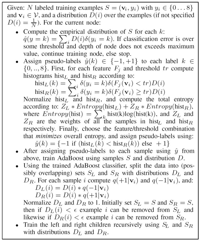
A brief description of the training procedure for PBT multiclass classifier [21].

After a PBT classifier is trained based on the procedures described in Fig. (4), the posterior p(y = k|v) can be computed recursively (this is an approximation). If the tree has no children, the posterior is simply the learned empirical distribution at the node p(y = k|v) = q̂(y = k). Otherwise the posterior is defined as:

$$p(y=k|\mathbf{v})=q(+1|\mathbf{v})p_R(y=k|\mathbf{v})+q(-1|\mathbf{v})p_L(y=k|\mathbf{v}).$$ (10)

Here q(y|v) is the posterior of the AdaBoost classifier, and p_L(y = k|v) and p_R(y = k|v) are the posteriors of the left and right trees, computed recursively. We can avoid traversing the entire tree by approximating p_L(y = k|v) with q̂_L(y = k) if q(−1|v) is small, and likewise for the right branch. Typically, using this approximation, only a few paths in the tree are traversed. Thus the amount of computation to calculate p(y|v) is roughly linear in the depth of the tree, and in practice can be computed very quickly.

B. Learning Generative Shape Models

Shape analysis has been one of the most studied topics in computer vision and medical imaging. Some typical approaches in this domain include Principal Component Analysis (PCA) shape models [22], [5], [23], the medial axis representation [7], and spherical wavelets analysis [27]. Despite the progress made [28], the problem remains unsolved. 3D shape analysis is very difficult for two reasons: (1) there is no natural order of the surface points in 3D, whereas one can use a parametrization to represent a closed contour in 2D, and (2) the dimension of a 3D shape is very high.

In this paper, a simple PCA shape model is adopted based on the signed distance function of the shape. A signed distance map is similar to the level sets representation [29] and some existing work has shown the usefulness of building PCA models on the level sets of objects [5]. In our hybrid models, much of the local shape information has already been implicitly fused in the discriminative appearance model, however, a global shape prior helps the segmentation by introducing explicit shape information. Experimental results with and without shape prior are shown in Table (III).

TABLE III.

Results on the test data using different combinations of the energy terms in Eqn. (4). Note that the results obtained using E_PCA are initialized from ground truth.

	LH	RH	LC	RC	LP	RP	LV	RV	Av
Recall	79%	69%	83%	77%	72%	72%	88%	85%	78%
Precis.	63%	51%	78%	77%	60%	68%	82%	82%	70%
(a) Results using EAP only
	LH	RH	LC	RC	LP	RP	LV	RV	Av
Recall	76%	67%	81%	77%	71%	70%	90%	89%	78%
Precis.	70%	57%	83%	84%	69%	74%	82%	81%	75%
(b) Results using EAP + ESM only
	LH	RH	LC	RC	LP	RP	LV	RV	Av
Recall	79%	79%	87%	86%	86%	87%	96%	97%	87%
Precis.	51%	50%	45%	46%	56%	62%	95%	95%	63%
(c) Results using EPCA only, with initialization from ground truth.

Our global shape model is simple and general. The same procedure is used to learn the shape models for 6 anatomical structures, namely, the left hippocampus (LH), right hippocampus (RH), left caudate (LC), right caudate (RC), left putamen (LP), and right putamen (RP). We do not apply the shape model to the background or the left ventricle (LV) or right ventricle (RV). The background is too irregular, while the ventricles often have elongated structures and their shapes are not described well by the PCA shape models. On the other hand, ventricles tend to be quite dark in many MRI volumes which makes the task of segmenting them relatively easier.

The volumes are registered and each anatomical structure is manually delineated by an expert in each of the MRI volumes, details are given in Section V. Basically, Brain volumes were roughly aligned and linearly scaled (Talairach and Tournoux 1988). Four control points were manually given to perform global registration followed by the algorithm [30] to perform 9 parameter registration. In this work n = 14 volumes were used for training. Let $R_k^1,\dots ,R_k^n$ denote the n delineated training samples for region R_k. First the center of each sample Rⁱ is computed (subscript dropped for convenience), and the centers for each i are aligned. Next, the signed distance map (SDM) Sⁱ is computed for each sample, where Sⁱ has the same dimensions as the original volume and the value of Sⁱ(a) is the signed distance of the voxel a to the surface of Rⁱ.

We apply PCA to S¹,…, Sⁿ. Let S̄ be the the mean SDM, and Q be a matrix with each column being a vectorized sample Sⁱ − S̄. We compute its singular value decomposition Q = UΣV^T. Now, the PCA coefficient of S (here we drop the superscript for convenience) are given by its projection β = U^T (S − S̄), and the corresponding probability of the shape according to the Gaussian model is:

$$p(S)\propto \mathit{exp}\left(-\frac{1}{2}{\beta }^T\sum \beta \right)$$ (11)

Note that n = 14 training shapes is very limited compared to the enormously large space in which all possible 3D shapes may appear. We keep the components of U whose corresponding eigenvalues are bigger than a certain threshold; in the experiments we found that setting the threshold such that 12 components are kept gives good results. Finally, note that a shape may be very different from the training samples but can still have a large probability since the probability is computed based on its projection onto the PCA space. Therefore, we add a reconstruction term to penalize unfamiliar shape: ∥(I − UU^T)(S − S̄)∥², where I is the identity matrix. The second energy term in Eqn. (4) becomes:

$$E_{\mathit{PCA}}=\sum _{k=1}^6\frac{1}{2}{\beta }_k^T{\sum }_k{\beta }_k+{\alpha }_3{\Vert (I-U_k{U}_k^T)(S_k-{\overline{S}}_k)\Vert }^2.$$ (12)

Fig. (7) shows a PCA shape model learned for the left hippocampus; it roughly captures the global shape regularity for the anatomical structures. Table (III) shows some experimental results with and without the PCA shape models, and we see improvements in the segmentations with the shape models. To further test the importance of the term E_PCA, we initialize our algorithm from the ground truth segmentation and then perform surface evolution based on shape only; we show results in Table (III) and Fig. (10). Due to the limited number of training samples and the properties of the PCA shape model itself, results are far from perfect. Learning a better shape model is one of our future research directions.

Fig. 7.

The PCA shape model learned for the left hippocampus. The shapes of the surface are shown at zero distance. The top-left figure shows the mean shape, the first three major components are shown in the top-right and bottom-right, and three random samples drawn from the PCA models (synthesized) are displayed in the bottom-left.

Fig. 10.

Results on a typical test volume. Three planes are shown overlayed with the boundaries of the segmented anatomical structures. The first row shows results manually labeled by an expert. The second row displays the result of using only the E_AP energy term. The third row shows the result of using E_AP and E_SM. The result in the fourth was obtained by initializing the algorithm from the ground truth and using E_PCA only. The result of our overall algorithm is displayed in the fifth row. The last row shows the result obtained using FreeSurfer [4].

The term E_PCA enforces the global shape regularity for each anatomical structure. Another energy term is added to encourage smooth surfaces:

$$E_{\mathit{SM}}=\sum _{k=0}^8{\mathit{\int }}_{\partial R_k}\mathit{dA},$$ (13)

Where ∫_∂Rk dA is the area of the surface of region R_k. When the total energy is being minimized in a variational approach [31], [32], this term corresponds to the force that encourages each boundary point to have small mean curvature, resulting in smooth surfaces (see appendix for the details).

C. Learning to Combine The Models

Once we have learned E_AP, E_PCA, and E_SM, we learn the optimal weights ${\alpha }_1^{\ast }$ and ${\alpha }_2^{\ast }$ to combine them. For any choice of α₁ and α₂, for each volume Vⁱ in the training set we can use the energy minimization approach from Section IV to compute the minimal solution Ŵⁱ(α₁,α₂) of E(W, V). Different choices of α₁ and α₂ will result in different segmentations, the idea is to pick the weights so that the segmentations of the training volumes are as good as possible.

Let ∥Wⁱ − Ŵⁱ(α₁, α₂)∥ measure the similarity between the segmentation result under the current (α₁, α₂) and the ground truth on volume Vⁱ. In this paper, we use precision-recall [33] to measure the similarity between two segmentations. One can adopt other approaches, e.g. Hausdorff distance [28], depending upon the emphasis on the errors. Our goal is to minimize:

$$({\alpha }_1^{\ast },{\alpha }_2^{\ast })=\arg \underset{({\alpha }_1,{\alpha }_2)}{\min }\sum _i\Vert W^i-{\widehat{W}}^i({\alpha }_1,{\alpha }_2)\Vert .$$ (14)

We solve for ${\alpha }_1^{\ast }$ and ${\alpha }_2^{\ast }$ using a steepest descent algorithm so that the segmentation results for all the training volumes are as close as possible to the ground truth.

IV. Segmentation Algorithm

In Section II we defined E(W, V) and in Section III we showed how to learn the shape and appearance models and how to combine them into our hybrid model. These were the modeling problems, we now turn to the computing issue, specifically, how to infer the optimal segmentation which minimizes the energy (4) given a novel volume V. We begin by introducing the motion equations used to perform surface evolution for segmenting sub-cortical structures. Next we discuss an explicit topology representation and then show how to use it to perform surface evolution. We end this Section with an outline of the overall algorithm.

A. Motion Equations

The goal in the inference/computing stage is to find the optimal segmentation which minimizes the energy in Eqn. (4). In our problem, the number of anatomical structures is known, as are their approximate positions. Therefore, we can apply a variational method to perform energy minimization. We adopt a surface evolution method [34] to perform surface evolution to minimize the energy E(W, V) in Eqn. (4). The original surface evolution method is in 2D, here we give the extended motion equations for E_AP, E_PCA, and E_SM in 3D. For more background information we refer readers to [34], [31]. Here we give the motion equations for the continuous case, derivations are given in the Appendix.

Let M be a surface point between region R_i and R_j. We can compute the effect of moving M on the overall energy by computing $\frac{d{E}_{\mathit{AP}}}{d\mathbf{M}}$, $\frac{d{E}_{\mathit{PCA}}}{d\mathbf{M}}$ and $\frac{d{E}_{\mathit{SM}}}{d\mathbf{M}}$. We begin with the appearance term:

$$\frac{d{E}_{\mathit{AP}}}{d\mathbf{M}}=-[\log \frac{p(y=i|\mathbf{V}(N(\mathbf{M}))}{p(y=j|\mathbf{V}(N(\mathbf{M}))}]\mathbf{N},$$ (15)

where N is the surface normal direction at M. Moving in the direction of the gradient $\frac{d{E}_{\mathit{AP}}}{d\mathbf{M}}$ allows each voxel to better fit the output of the discriminative model. Effect on the global shape model is:

$$\frac{d{E}_{\mathit{PCA}}}{d\mathbf{M}}=-{\alpha }_1\left[\left({\beta }_i^T{\sum }_i-2{\alpha }_3{(S_i-{\overline{S}}_i)}^T(I-U_i{U}_i^T)\right)J_i(\mathbf{M})-({\beta }_j^T{\sum }_j-2{\alpha }_3{(S_j-{\overline{S}}_j)}^T(I-U_j{U}_j^T))J_j(\mathbf{M})\right]\mathbf{N}.$$ (16)

J_i(M) and J_j(M) are the Jacobian matrices for the signed distance map for R_i and R_j respectively. Finally, the motion equation derived from the smoothness term is:

$$\frac{d{E}_{\mathit{SM}}}{d\mathbf{M}}=-{\alpha }_{2}H\mathbf{N},$$ (17)

where H is the curvature at M.

Eqn. (15) contributes to the force in moving the boundary to better fit the classification model, Eqn. (16) contributes to the force to fit the global shape model, and Eqn. (17) favors small curvature resulting in smoother surfaces. The final segmentation is a result of balancing each of the above forces: (1) each region should contain voxels that match its appearance model p(y|V(N(M)), (2) the overall shape of each anatomical structure should have high probability, and (3) the surfaces should be locally smooth. Results using different combinations of these terms are shown in Fig. (10) and Table (III).

B. Grid-Face Representation

In order to apply the motion equations to perform surface evolution, an explicit representation of the regions in necessary. 3D shape representation is a challenging problem. Some popular methods include parametric representations [35] and finite element representations [6]. The joint priors defined in [5] are used to prevent the surfaces of different objects from intersecting with each other in the level set representation. The level set method [29] implicitly handles region topology changes, and has been widely used in image segmentation. However, the sub-cortical structures in 3D brain images are often topologically connected, which introduces difficulty in the level set implementation.

In this paper, we propose a grid-face representation to explicitly code the region topology. We take advantage of the particular form of our problem: we are dealing with a fixed number of topologically connected regions that are non-overlapping and together include every voxel in the volume. Recall from Eqn. (1) that we can represent a segmentation as W = {R₀,…, R₈}, where each R_i stores which voxels belong to region i. If we think of each voxel as a cube, then the boundary between two adjacent voxels is a square, or face. The grid-face representation G of a segmentation W is the set of all faces whose adjacent voxels belong to different regions. It is worth to mention that although the shape prior is defined by a PCA model for each structure separately, the actual region topology is maintained by the grid-face representation, which is a full partition of the lattice. Therefor, regions will not overlap to each other.

The resulting representation is conceptually simple and facilitates fast surface evolution. It can represent an arbitrary number of regions and maintains a full partition of the input volume. By construction, regions may be adjacent but cannot overlap. Fig. (8) shows an example of the representation; it bears some similarity with [36]. It has some limitations, for example sub-voxel precision cannot be achieved. However, this does not seem to be of critical importance in 3D brain images, and the smoothness term in the total energy prevents the surface from being too jagged.

Fig. 8.

Illustration of the grid-face representation. Left: To code the region topology, a label map is stored in which each voxel is assigned with the label of the anatomical structure to which the voxel currently belongs. Middle: Surface evolution is applied to a single slice of the volume, either along an X-Y, Y-Z, or X-Z plane. Shown is the middle slice along the X-Y plane. Right: Forces are computed using the motion equations at face M, which lies between voxels a₁ and a₂. The sum of the forces causes M to move to M′, resulting in a change of ownership of a₁ from R₁ to R₀. Top/Bottom: G before and after application of forces to move M.

C. Surface Evolution

Applying the motion equations to the grid-face representation G is straightforward. The motion equations are defined for every point M on the boundary between two regions, and in our representation, each face in G is a boundary point. Let a₁ and a₂ be two adjacent voxels belonging to two different regions, and M the face between them. Each of the forces works along the surface normal N. If the magnitude of the total force is bigger than 1 then the face M may move 1 voxel to the other side of either a₁ or a₂, resulting in the change of the ownership of the corresponding voxel. The move is allowed so long as it does not result in a region becoming disconnected. Fig. (8) illustrates an example of a boundary point M moving 1 voxel.

To perform surface evolution, we visit each face M in turn, apply the motion equations and update G accordingly. Specifically, we take a 2D slice of the 3D volume along an X -Y, Y -Z, or X-Z plane, and then perform one move on each of the boundary points in the slice. Essentially, the problem of 3D surface evolution is reduced to boundary evolution in 2D, see Fig. (8). During a single iteration, each 2D slice of the volume is visited once; we perform a number of such iterations, either until G does not change or a maximum number of iterations is reached.

D. Outline of The Algorithm

Training

1. For a set of training volumes with the anatomical structures manually delineated, train multi-class PBT to learn the discriminative model p(y|V(N(a)) as described in Section III-A.

2. For each anatomical structure learn its PCA shape model as discussed in Section III-B

3. Learn α₁ and α₂ to combine the discriminative and generative models as described in Section III-C.

Segmentation

1. Given an input volume V, compute p(y|V(N(a)) for each voxel a.

2. Assign each voxel in V with the label that maximizes p(y|V(N(a)). Based on this classification map, we use a simple morphological operator to find all the connected regions. In each individual region, all the voxels are 6-neighborhood connected and they have the same label. Note that at this stage two disjoint regions may have the same label. For all the regions with the same label (except 0), we only keep the biggest one and assign the rest to the background. Therefore, we obtain an initial segmentation W in which all 8 anatomical structures are topologically connected.

3. Compute the initial grid-face representation G based on W as described in Section IV-B. Perform surface evolution as described in Section IV-C to minimize the total energy E(W, V) in Eqn. (4).

4. Report the final segmentation result W.

V. Experiments

High-resolution 3D SPGR T1-weighted MR images were acquired on a GE Signa 1.5T scanner as a series of 124 contiguous 1.5 mm coronal slices (256×256 matrix; 20cm FOV). Brain volumes were roughly aligned and linearly scaled (Talairach and Tournoux 1988). Four control points were manually given to perform global registration followed by the algorithm [30] to perform 9 parameter registration. This procedure is used to correct for differences in head position and orientation and places data in a common co-ordinate space that is specifically used for inter-individual and group comparisons. All the volumes shown in the paper are registered using the above procedure.

Our dataset includes 28 volumes annotated by neuroanatomists. The volumes were split in half randomly, 14 volumes were used for training and 14 for testing. The training and testing processes was repeated twice and we observed the same performances. The training volumes together with the annotations are used to train the discriminative model introduced in Section III-A and the generative shape model discussed in Section III-B. After, we apply the algorithm described in Section IV to segment the eight anatomical structures in each volume. Computing the discriminative appearance model is fast (a few minutes per volume) due to hierarchical structure of PBT and the use of integral volume. It takes an additional 5 minutes to perform surface evolution to obtain the segmentation, for a total of 8 minutes per volume.

Results on a test volume are shown in Fig. (10), along with the corresponding manual annotation. Qualitatively, the anatomical structures are segmented correctly in most places, although not all the surfaces are precisely located. The results obtained by our algorithm are more regular (less jagged) than human labels. The results on the training volumes (not shown) are slightly better than those on the test volumes, but the differences are not large.

To quantitatively measure the effectiveness of our algorithm, errors are measured using several popular criteria, including Precision-Recall [33], Mean distance [5], and Hausdorff distance [28]. Let R be the set of voxels annotated by an expert and R̂ be the voxels segmented by the algorithm. These three error criteria are defined, respectively, as:

$$\mathit{Precision}=\frac{R\cap \widehat{R}}{\widehat{R}};\mathit{Recall}=\frac{R\cap \widehat{R}}{R}$$ (18)

$$d_M(R,\widehat{R})=\frac{1}{\mid R\mid }\sum _{s\in R}{\mathit{min}}_{b\in \widehat{R}}\Vert s-b\Vert .$$ (19)

$$d_H(R,\widehat{R})=\mathit{in}f\{\in >0|R\subseteq {\widehat{R}}^{\mathit{\in }}\}$$ (20)

In the definition of d_H, R̂^∈ denotes the union of all disks with radius ∈ centered at a point in R̂. Finally, note that d_H is an asymmetric measure.

Table (II) shows the precision-recall measure [33] on the training and test volumes for each of the eight anatomical structures, as well as the overall average precision and recall. The test error is slightly worse than the training error, but again the differences are not large. To directly compare our algorithm to an existing state of the art method, we tested the MRI data using FreeSurfer [4], and our results are slightly better. We also show segmentation results by FreeSurfer in the last row of Fig. (10); since FreeSurfer uses Markov Random Fields (MRF) and lacks explicit shape information, the segmentation results were more jagged. Note that FreeSurfer segments more subcortical structures than our algorithm, and we only compare the results on those discussed in this paper.

TABLE II.

Precision and recall measures for the results on the training and test volumes. The test error is only slightly worse than the training error, which says that the algorithm generalizes well. We also test the same set of volumes using FreeSurfer [4], our results are slightly better.

	LH	RH	LC	RC	LP	RP	LV	RV	Av
Recall	69%	68%	86%	84%	79%	78%	91%	91%	81%
Precis.	78%	72%	85%	85%	70%	78%	82%	82%	79%
(a) Results on the training data
	LH	RH	LC	RC	LP	RP	LV	RV	Av
Recall	69%	62%	84%	81%	75%	75%	90%	90%	78%
Precis.	77%	64%	81%	83%	68%	72%	81%	81%	76%
(b) Results on test data
	LH	RH	LC	RC	LP	RP	LV	RV	Av
Recall	66%	84%	77%	77%	83%	83%	76%	76%	78%
Precis.	47%	54%	78%	78%	71%	77%	81%	72%	70%
(c) Results on the test data by FreeSurfer [4]

Table (IV) shows the Hausdorff and Mean distances between the segmented anatomical structures and the manual annotations on both the training and test sets; smaller distances are better. The various error measure are quite consistent – the hippocampus and putamen are among the hardest to accurately segment while the ventricles are fairly easy due to their distinct appearance. For the asymmetric Hausdorff distance we show both d_H(R̂, R) and d_H(R, R̂). For the Mean distance we give the standard deviation, which was also reported in [5]. On the same task, Yang et al. [5] reported a mean error of 1.8 and a variation of 1.2, however, the results are not directly comparable because the datasets are different and their error was computed using the the leave-one-out method with 12 volumes in total. Finally, we note that the running time of our algorithm, approximately 8 minutes, is around 20 to 30 times faster then theirs (which takes a couple of hours per volume). The speed advantage of our algorithm is due to: (1) efficient computation of the discriminative model using a tree structure, (2) fast feature computation based on integral volumes, and (3) variational approach of surface evolution on the grid-face representation.

TABLE IV.

(a,b) Hausdorff Distances for the results on the training and test volumes; the measure is in terms of voxels. (c,d) Mean distance measures for the results on the training and test volumes.

	LH	RH	LC	RC	LP	RP	LV	RV	Av
dH(R̂, R)	6.6	10.0	6.6	5.0	10.4	8.6	5.6	6.0	7.4
dH(R, R̂)	10.4	11.9	7.9	8.6	10.3	9.7	16.0	13.9	11.1
(a) Results on training data measured using Hausdorff distance
	LH	RH	LC	RC	LP	RP	LV	RV	Av
dH(R̂, R)	6.7	14.3	8.0	6.7	10.2	10.1	6.3	6.9	8.7
dH(R, R̂)	12.1	13.6	8.1	8.5	10.6	9.4	11.4	14.7	11.1
(b) Results on test data measured using Hausdorff distance
	LH	RH	LC	RC	LP	RP	LV	RV	Av
mean	1.8	2.2	1.3	1.3	2.5	2.0	1.1	1.0	1.7
σ	0.53	0.52	0.24	0.36	0.78	0.39	0.38	0.13	0.4
(c) Results on training data measured using Mean Distance
	LH	RH	LC	RC	LP	RP	LV	RV	Av
mean	2.0	2.8	1.5	1.4	2.6	2.4	1.1	1.1	1.9
σ	0.37	1.1	0.33	0.29	0.83	0.76	0.26	0.24	0.5
(d) Results on test data measured using Mean Distance

To demonstrate how each energy term in Eqn. (4) affects the quality of the final segmentation, we also test our algorithm using E_AP only, E_AP and E_SM, and E_PCA. To be able to test using shape only, we initialize the segmentation to the ground truth and then perform surface evolution based on the E_PCA term only. Although imperfect, this procedure allows us to see whether E_PCA on its own is doing something reasonable. Results can be seen in the second, third and forth row in Fig. (10) and we report precision and recall in Table (III). We make the following observations: (1) The sub-cortical structures can be segmented fairly accurately using E_AP only. This shows a sophisticated model of appearance can provide significant information for segmentation. (2) The surfaces are much smoother by adding the E_SM on the top of E_AP, and we also see improved results in terms of errors. (3) The PCA models are able to roughly capture the global shapes of the sub-cortical structures, but only improve the overall error slightly. (4) The best set of results are obtained by including all three energy terms.

We also asked an independent expert trained on annotating sub-cortical structures to rank these different approaches based on the segmentation results. The ranking from the best to the worst are respectively: Manual, E, E_AP + E_SM, E_AP, FreeSurfer, E_PCA. This echoes the error measures obtained in Table (II) and Table (III).

As stated in Section IV-D, we start the 3D surface evolution from an initial segmentation based on the discriminative appearance model. To test the robustness of our algorithm, we also started the method from the small seed regions shown in Fig. (9). Several steps in the surface evolution process are shown. The algorithm quickly converges to nearly the identical result as shown in Fig. (10), even though it was initialized very differently. This demonstrates that our approach is robust and the final result does not depend heavily on the initial segmentation. The algorithm does, however, converge faster if it starts from a good initial state.

Fig. 9.

Results on a test volume with the segmentation algorithm initialized with small seed regions. The algorithm quickly converges to the final result. The final segmentation are nearly the identical result as those shown in Fig. 10, where the initial segmentations were obtained based on the classification result of the discriminative model. This validates the hybrid discriminative/generative models and it also demonstrates the robustness of our algorithm.

VI. Conclusion & Future Work

In this paper, we proposed a system for brain anatomical structure segmentation using hybrid discriminative/generative models. The algorithm is very general, and easy to train and test. It has very few parameters that need manual specification (only a couple of generic ones in training PBT, e.g. the depth of the tree), and it is quite fast – taking on the order of minutes to process an input 3D volume.

We evaluate our algorithm both quantitatively and qualitatively, and the results are encouraging. A comparison between our algorithm using different combinations of the energy terms and FreeSurfer is given. Compared to FreeSurfer, our system is much faster and the results obtained are slightly better. However, FreeSurfer is able to segment more sub-cortical structures. A full scale comparison with other existing state of art algorithms needs to be done in the future.

We emphasize the learning aspect of our approach for integrating the discriminative appearance and generative shape models closely. The system makes use of training data annotated by experts and learns the rules implicitly from examples. A PBT framework is adopted to learn a multi-class discriminative appearance model. It is up to the learning algorithm to automatically select and combine hundreds of cues such as intensity, gradients, curvatures, and locations to model ambiguous appearance patterns of the different anatomical structures. We show that pushing the low-level (bottom-up) learning helps resolve a large amount of ambiguity, and engaging the generative shape models further improves the results slightly. Discriminative and generative models are naturally combined in our learning framework. We observe that: (1) the discriminative model plays the major role in obtaining good segmentations; (2) the smoothness term further improves the segmentation; and (3) the global shape model further constrains the shapes but improves results only slightly.

We hope to improve our system further. We anticipate that the results can be improved by: (1) using more effective shape priors, (2) learning discriminative models from a bigger and more informative feature pool, and (3) introducing an explicit energy term for the boundary fields.

Fig. 3.

A brief description of the AdaBoost training procedure [24].

Appendix: Derivation of Motion Equations

Here we give detailed proofs for the motion equations (Eqn. (15) and Eqn. (17)). For notational clarity, we write the equations in the continuous domain, and their numerical implementations are just approximations in a discretized space. Let M = (x(u, v), y(u, v), z(u, v)) be a 3D boundary point, and let R be a region and ∂R = S its corresponding surface.

Motion equation for E_AP

The discriminative model for each region R_k is

$$-{\mathit{\int }}_{R_k}\mathit{log}(p(y=k|\mathbf{V}(N(\mathbf{M}))\mathit{da},$$ (21)

as given in Eqn. (5). A derivation of the motion equation in the 2D case, based on Green’s theorem and Euler-Lagrange equation, can be found in [34]. Now we show a similar result for the 3D case. The Curl theorem [37] says

$${\mathit{\int }}_R(\nabla ·\mathbf{F})\mathit{da}={\mathit{\int }}_{\partial R}\mathbf{F}\mathit{dA}$$

where F : ℜ³ → ℜ³ and ∇ · F is the divergence of F, which is a scalar function on ℜ³. Therefore, the motion equation for the above function on a surface point M ∈ ∂R can be readily obtained by the Euler-Lagrange equation as

$$-(\nabla ·\mathbf{F})\mathbf{N},$$

where N is the normal direction of M on ∂R. In our case, every point M on the surface ∂R_i is also on the surface ∂R_j of its neighboring region R_j. Thus, the overall motion equation for the discriminative model is

$$\frac{d{E}_{\mathit{AP}}}{d\mathbf{M}}=-[\log \frac{p(y=i|\mathbf{V}(N(\mathbf{M}))}{p(y=j|\mathbf{V}(N(\mathbf{M}))}]\mathbf{N}.$$

Motion equation for E_SM

The motion equation for a term similar to E_SM was shown in [32] and more clearly illustrated in [31]. To make this paper self-contained, we give the derivation here also. For region R,

$$E_{\mathit{SM}}={\mathit{\int }}_{\partial R}\mathit{dA}=\mathit{\iint }\sqrt{\mathit{EG}-F^2}\mathit{dudv}$$

where

$$E={(\frac{\partial x}{\partial u})}^2+{(\frac{\partial y}{\partial u})}^2+{(\frac{\partial z}{\partial u})}^2,$$

$$F=(\frac{\partial x}{\partial u})(\frac{\partial x}{\partial v})+(\frac{\partial y}{\partial u})(\frac{\partial y}{\partial v})+(\frac{\partial z}{\partial u})(\frac{\partial z}{\partial v}),$$

and

$$G={(\frac{\partial x}{\partial v})}^2+{(\frac{\partial y}{\partial v})}^2+{(\frac{\partial z}{\partial v})}^2.$$

$$\begin{array}{ll}\frac{\partial }{\partial t}{\mathit{\int }}_{\partial R}\mathit{dA}& =\mathit{\iint }\sqrt{\mathit{EG}-F_t^2}\mathit{dudv}\\ & =\mathit{\iint }\frac{E_{t}G+G_{t}E-2F{F}_t}{2\sqrt{\mathit{EG}-F^2}}\mathit{dudv}\\ & =\mathit{\iint }\frac{2G\langle {\mathbf{M}}_{\mathit{ut}},{\mathbf{M}}_u\rangle +2E\langle {\mathbf{M}}_{\mathit{vt}},{\mathbf{M}}_v\rangle -2F\left(\langle {\mathbf{M}}_{\mathit{vt}},{\mathbf{M}}_u\rangle +\langle {\mathbf{M}}_{\mathit{ut}},{\mathbf{M}}_v\rangle \right)}{2\sqrt{\mathit{EG}-F^2}}\mathit{dudv}\\ & =\mathit{\iint }-\frac{\langle G{\mathbf{M}}_{\mathit{uu}},{\mathbf{M}}_t\rangle +E\langle {\mathbf{M}}_{\mathit{vv}},{\mathbf{M}}_t\rangle -2F\langle {\mathbf{M}}_{\mathit{uv}},{\mathbf{M}}_t\rangle }{\sqrt{\mathit{EG}-F^2}}\mathit{dudv}\\ & =\mathit{\iint }-\frac{\langle G\langle {\mathbf{M}}_{\mathit{uu}},\mathbf{N}\rangle \mathbf{N}+E\langle {\mathbf{M}}_{\mathit{vv}},\mathbf{N}\rangle \mathbf{N}-2F\langle {\mathbf{M}}_{\mathit{uv}},\mathbf{N}\rangle \mathbf{N},{\mathbf{M}}_t\rangle }{\sqrt{\mathit{EG}-F^2}}\mathit{dudv}\\ & =\mathit{\iint }\langle -2H\mathbf{N},{\mathbf{M}}_t\rangle \sqrt{\mathit{EG}-F^2}\mathit{dudv}\\ & =\mathit{\iint }\langle -2H\mathbf{N},{\mathbf{M}}_t\rangle \mathit{dA}\end{array}$$

Letting M_t = HN leads to the decrease in the energy. Thus, the motion equation for E_SM is:

$$\frac{d{E}_{\mathit{SM}}}{d\mathbf{M}}=-{\mathbf{M}}_t=-H\mathbf{N},$$

where H is the mean curvature and N denotes the normal direction at M.

References

- 1.Pohl KM, Fisher J, Kikinis R, Grimson WEL, Wells WM. A bayesian model for joint segmentation and registration. Medical Image Analysis. 2004;8:275–283. [Google Scholar]
- 2.Narr KL, Thompson PM, Sharma T, Moussai J, Blanton R, Anvar B, Edris A, Krupp R, Rayman J, Khaledy M, Toga AW. Three-dimensional mapping of temporo-limbic regions and the lateral ventricles in schizophrenia: gender effects. Biol Psychiatry. 2001;50(2):84–97. doi: 10.1016/s0006-3223(00)01120-3. [DOI] [PubMed] [Google Scholar]
- 3.Sowell ER, Trauner DA, Gamst A, Jernigan TL. Development of cortical and subcortical brain structures in childhood and adolescence: a structural mri study. Developmental Medicine Child Neurology. 2002 Jan;44(1):4–16. doi: 10.1017/s0012162201001591. [DOI] [PubMed] [Google Scholar]
- 4.Fischl B, Salat DH, Busa E, Albert M, Dieterich M, Haselgrove C, van der Kouwe A, Killiany R, Klaveness S, Kennedy D, Montillo A, Makris N, Rosen B, Dale AM. Whole brain segmentation: automated labeling of neuroanatomical structures in the human brain. Neuron. 2002;33:341–355. doi: 10.1016/s0896-6273(02)00569-x. [DOI] [PubMed] [Google Scholar]
- 5.Yang J, Staib LH, Duncan JS. Neighbor-constrained segmentation with level set based 3d deformable models. IEEE Trans on Medical Imaging. 2004 Aug;23(8):940–948. doi: 10.1109/TMI.2004.830802. [DOI] [PMC free article] [PubMed] [Google Scholar]
- 6.Pohl KM, Fisher J, Kikinis R, Grimson WEL, Wells WM. A bayesian model for joint segmentation and registration. NeuroImage. 2006;31(1):228–239. doi: 10.1016/j.neuroimage.2005.11.044. [DOI] [PubMed] [Google Scholar]
- 7.Pizer SM, Fletcher T, Fridman Y, Fritsch DS, Gash AG, Glotzer JM, Joshi S, Thall A, Tracton G, Yushkevich P, Chaney EL. Deformable m-reps for 3d medical image segmentation. Int’l J of Comp Vis. 2003;55(2):85–106. doi: 10.1023/a:1026313132218. [DOI] [PMC free article] [PubMed] [Google Scholar]
- 8.Woolrich MW, Behrens TE. Variational bayes inference of spatial mixture models for segmentation. IEEE Trans on Medical Imaging. 2006 Oct;2(10):1380–1391. doi: 10.1109/tmi.2006.880682. [DOI] [PubMed] [Google Scholar]
- 9.Li C, Goldgof DB, Hall LO. Knowledge-based classification and tissue labeling of mr images of human brain. IEEE Trans on Medical Imaging. 1993 Dec;12(4):740–750. doi: 10.1109/42.251125. [DOI] [PubMed] [Google Scholar]
- 10.Rohlfing T, Russakoff DB, Maurer CR., Jr Performance-based classifier combination in atlas-based image segmentation using expectation-maximization parameter estimation. IEEE Trans on Medical Imaging. 2004 August;23(8):983–994. doi: 10.1109/TMI.2004.830803. [DOI] [PubMed] [Google Scholar]
- 11.Descombes X, Kruggel F, Wollny G, Gertz HJ. An object-based approach for detecting small brain lesions: application to virchow-robin spaces. IEEE Tran on Medical Img. 2004 Feb;23(2):246–255. doi: 10.1109/TMI.2003.823061. [DOI] [PubMed] [Google Scholar]
- 12.Lao Z, Shen D, Jawad A, Karacali B, Liu D, Melhem E, Bryan N, Davatzikos C. Proc of 3rd IEEE In’l Symp on Biomedical Imaging (ISBI) Arlington: Apr, 2006. Automated segmentation of white matter lesions in 3d brain mr images, using multivariate pattern classification; pp. 307–310. [Google Scholar]
- 13.Lee CH, Schmidt M, Murtha A, Bistritz A, Sander J, Greiner R. Proc of Workshop of Comp Vis for Biomedical Image App : Current Techniques and Future Trends. Beijing: Oct, 2005. Segmenting brain tumor with conditional random fields and support vector machines; pp. 469–478. [Google Scholar]
- 14.Tu Z, Zhou XS, Comaniciu D, Bogoni L. A learning based approach for 3d segmentation and colon detagging. Proc of Europ Conf on Comp Vis (ECCV) 2006 May;:436–448. [Google Scholar]
- 15.Cocosco C, Zijdenbos A, Evans A. A fully automatic and robust brain mri tissue classification method. Medical Image Analysis. 2003 Dec;7(4):513–527. doi: 10.1016/s1361-8415(03)00037-9. [DOI] [PubMed] [Google Scholar]
- 16.Wyatt PP, Noble JA. Map mrf joint segmentation and registration. Proc of 10th Int’l Conf on Medical Image Computing and Computer Assisted Intervention (MICCAI) 2002 Oct;:580–587. [Google Scholar]
- 17.Heckemann RA, Hajnal JV, Aljabar P, Rueckert D, Hammers A. Automatic anatomical brain mri segmentation combining label propagation and decision fusion. Neuroimage. 2006 Oct;33(1):115–126. doi: 10.1016/j.neuroimage.2006.05.061. [DOI] [PubMed] [Google Scholar]
- 18.Liu Y, Teverovskiy L, Carmichael O, Kikinis R, Shenton M, Carter CS, Stenger VA, Davis S, Aizenstein H, Becker J, Lopez O, Meltzer C. Discriminative mr image feature analysis for automatic schizophrenia and alzheimer’s disease classification. Proc of Int’l Conf on Medical Image Computing and Computer Assisted Intervention (MICCAI) 2004 Oct;:393–401. [Google Scholar]
- 19.Lafferty J, McCallum A, Pereira F. Proc of 10th Int’l Conf on Machine Learning. San Francisco: 2001. Conditional random fileds: probabilistic models for segmenting and labeling sequence data; pp. 282–289. [Google Scholar]
- 20.Raina R, Shen Y, Ng AY, McCallum A. Classification with hybrid generative/discriminative models. Proc of Neuro Information Processing Systems (NIPS) 2003 [Google Scholar]
- 21.Tu Z. Proc of Int’l Conf on Comp Vis (ICCV) Beijing: Oct, 2005. Probabilistic boosting tree: Learning discriminative models for classification, recognition, and clustering; pp. 1589–1596. [Google Scholar]
- 22.Cootes TF, Edwards GJ, Taylor CJ. Computerized brain tissue classification of magnetic resonance images: A new approach to the problem of partial volume artifact. IEEE Tran on Patt Anal and Mach Intel. 2001 June;23(6):681–685. [Google Scholar]
- 23.Leventon ME, Grimson WEL, Faugeras O. Statistical shape influence in geodesic active contours. Proc of Comp Vis and Patt Recog. 2000 June;:316–323. [Google Scholar]
- 24.Freund Y, Schapire RE. A decision-theoretic generalization of on-line learning and an application to boosting. J of Comp and Sys Sci. 1997;55(1):119–139. [Google Scholar]
- 25.Friedman J, Hastie T, Tibshirani R. Additive logistic regression: a statistical view of boosting. Dept of Statistics, Stanford Univ Technical Report. 1998 [Google Scholar]
- 26.Dollár P, Tu Z, Tao H, Belongie S. IEEE Conf on Comp Vis and Patt Recog CVPR’2007. Minneapolis: Jun, 2006. Feature mining for image classification. [Google Scholar]
- 27.Nain D, Haker S, Bobick A, Tannenbaum A. Proc of Int’l Conf on Medical Image Computing and Computer Assisted Intervention (MICCAI) Copenhagen: Oct, 2006. Shape-driven 3d segmentation using spherical wavelets; pp. 66–74. [DOI] [PMC free article] [PubMed] [Google Scholar]
- 28.Loncaric S. A survey of shape analysis techniques. Pattern Recognition. 1998;31(8):983–1001. [Google Scholar]
- 29.Osher S, Sethian JA. Front propagating with curvature dependent speed: algorithms based on hamilton-jacobi formulation. J of Computational Physics. 1988;79(1):12–49. [Google Scholar]
- 30.Woods RP, Mazziotta JC, Cherry SR. Mri-pet registration with automated algorithm. Journal of Computer Assisted Tomography. 1993;17:536–546. doi: 10.1097/00004728-199307000-00004. [DOI] [PubMed] [Google Scholar]
- 31.Jin H. Ph.D. thesis. Dept of Elec Eng, Washington Univ; 2003. Variational method for shape reconstruction in computer vision. [Google Scholar]
- 32.Faugeras O, Keriven R. Variational principles, surface evolution pdes, level set methods and the stereo problem. IEEE Trans on Image Proc. 1998 March;7(3):336–344. doi: 10.1109/83.661183. [DOI] [PubMed] [Google Scholar]
- 33.Martin D, Fowlkes C, Malik J. Learning to detect natural image boundaries using local brightness, color and texture cues. IEEE Trans on Pattern Analysis and Machine Learning. 2004 May;26(5):530–549. doi: 10.1109/TPAMI.2004.1273918. [DOI] [PubMed] [Google Scholar]
- 34.Zhu SC, Yuille AL. Region competition: Unifying snake/balloon, region growing and bayes/mdl/energy for multi-band image segmentation. IEEE Trans on Pattern Analysis and Machine Learning. 1996 Sept;18(9):884–900. [Google Scholar]
- 35.Frangi AF, Rueckert D, Schnabel JA, Niessen WJ. Automatic construction of multiple-object three-dimensional statistical shape models: application to cardiac modeling. IEEE Tran on Medical Img. 2002 Sept;21(9):1151–1166. doi: 10.1109/TMI.2002.804426. [DOI] [PubMed] [Google Scholar]
- 36.Malandain G, Bertrand G, Ayache N. Topological segmentation of discrete surfaces. Int’l J of Comp Vis. 1993;10(2):183–197. [Google Scholar]
- 37.Arfken G. Mathematical Methods for Physicists. FL: Academic Press; 1985. [Google Scholar]