Analytical Method for the Fast Time-Domain Reconstruction of Fluorescent Inclusions In Vitro and In Vivo

Abstract

A novel time-domain optical method to reconstruct the relative concentration, lifetime, and depth of a fluorescent inclusion is described. We establish an analytical method for the estimations of these parameters for a localized fluorescent object directly from the simple evaluations of continuous wave intensity, exponential decay, and temporal position of the maximum of the fluorescence temporal point-spread function. Since the more complex full inversion process is not involved, this method permits a robust and fast processing in exploring the properties of a fluorescent inclusion. This method is confirmed by in vitro and in vivo experiments.

Introduction

Optical fluorescence imaging has the potential to provide clinical information in bioengineering applications such as tissue oxygenation, glucose levels, and small molecule protein-protein interactions (1) as well as the early detection of tumor cells. There are three major approaches to optical fluorescence imaging of a tissuelike turbid medium: continuous-wave (CW) intensity measurement using steady-state light source; frequency-domain (FD) technique using modulated light source; and time-domain (TD) technique using pulsed light source. The CW technique has been widely used, due to its simple and inexpensive implementation. CW techniques generally provide two-dimensional images of fluorescence intensity, whereas FD and TD techniques provide the fluorophore lifetime as well (2). Measuring a fluorescence temporal point-spread function (TPSF) (3) also enables an estimate of the fluorophore depth. Full tomographic methods have been developed in CW, FD, and TD where multiple source-detector pair measurements are required at many angles with complicated and highly intensive inversion processes (4). In addition to a single-point scanning scheme using a photomultiplier tube and time-correlated single-photon counting system (5), fluorescence lifetime imaging has been achieved with whole-field imaging using a time-gated charge-coupled device camera for faster measurement in tissue sections (6,7) and in a mouse in vivo (8).

Recently, Kumar et al. (9,10) presented a fluorescence tomography algorithm based on an asymptotic lifetime analysis of TD fluorescence signals. Laidevant et al. (11) presented a method for localizing a single fluorescence inclusion embedded in a homogeneous turbid medium. Hall et al. (3) presented a simple TD optical approach to estimating the depth and concentration of a fluorescent inclusion. In our recent publication (12), we suggested the simple TD optical method to estimate the lifetime and depth of a fluorescent inclusion in a turbid medium. For whole-body imaging, both fast acquisition and fast processing are needed for preclinical and clinical applications. Here, we will present a novel, to our knowledge, analytical method to reconstruct the relative concentration, lifetime, and depth of a fluorescent inclusion by the simple analysis of the fluorescence TPSF. To validate the method described in this work, we performed in vitro phantom studies and in vivo mouse experiments.

Methods

Optical probe

Cy7 (GE Healthcare, Piscataway, NJ) is a near-infrared fluorophore with peak excitation at 743 nm and a peak emission at 767 nm. The molecular structure of Cy7 and absorption/emission spectra are seen elsewhere (13). To expedite the repeated measurements, solid fluorescent pellets were manufactured according to a method described elsewhere (14).

Optical properties

In this work, we used Cy7 as a fluorophore and Intralipid-1% as a turbid medium at λ = 760 nm. The lifetime τ of solid Cy7 is 1 ns. According to van Staveren et al. (15), μ_a = 2.0 × 10⁻³ mm⁻¹, μ_s = (2.54 × 10⁸) · (λ [nm])^−2.4 mm⁻¹, and anisotropy factor g = 1.1 – (0.58 × 10⁻³) · (λ [nm]) for Intralipid-10%. Thus, for the Intralipid-1% that we used in this work, the optical properties of the medium is μ_s = 3.1 mm⁻¹ and g = 0.659, thus, μ′_s = μ_s(1 – g) = 1.05 mm⁻¹. The impulse response function (IRF) was independently measured and assumed to take the form of Gaussian, with t_IRF = 1.27 ns and σ_IRF = 0.24 ns.

In vivo fluorescence lifetime imaging

Time-resolved imaging was carried out using eXplore Optix-MX2 (ART Advanced Research Technologies, Montreal, Canada). The system uses a single source-detector configuration in the reflection mode. Detailed system information is described elsewhere (12). Schematic measurement geometry is depicted in Fig. 1. Scan step was 2 mm and scan time was 1 s for a collection at each point in the region of interest. Optix-MX2 uses the IRF measurement as a temporal reference to define the excitation time of the medium (t = 0).

Figure 1.

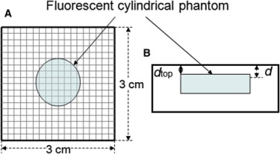
(A) Scanning geometry is composed of a source and a detector with 3-mm fixed separation and scans every 2 mm. The diameter and the thickness of this cylindrical phantom were 15 mm and 8 mm, respectively. The imaged area is 3 × 3 cm². (B) Side view of Fig. 1 A.

Histology

Nude mice were anesthetized (i.p. injection of 50 mg/Kg Ketamine and 1 mg/Kg Acepromazine) and tail vein intravenously injected (0.5 mL insulin syringe-28.5 gauge fixed needle) with a 0.1 mL dose of Cy7 at 10 μM concentration.

Theory

Light propagation model

Near-infrared light, incident on a highly scattering turbid medium, is governed by the diffusion equation for the diffuse photon fluence rate ϕ(r, t) (12,16):

$$-\nabla ·\left(D\left(\mathbf{r}\right)\nabla \mathit{\varphi }\left(\mathbf{r},t\right)\right)+\frac{1}{v}\frac{\partial \mathit{\varphi }\left(\mathbf{r},t\right)}{\partial t}+{\mathit{\mu }}_{\text{a}}\left(\mathbf{r}\right)\mathit{\varphi }\left(\mathbf{r},t\right)=S\left({\mathbf{r}}_{\text{s}},t\right)\text{.}$$ (1)

The diffusion equation has been employed by several researchers to address the fluorescence problem (9–11,17–19). The δ-response for light propagation in a turbid infinite medium is described by the Green's function (12,16,20),

$$G\left(\mathbf{r},t\right)=\frac{1}{{\left(4\pi Dvt\right)}^{3/2}}\exp \left(-\frac{r^2}{4Dvt}-{\mathit{\mu }}_{\text{a}}vt\right),$$ (2)

which is a solution to the diffusion equation under the assumption of the homogeneity of the absorption coefficient μ_a and the reduced coefficient μ′_s. Under these conditions and under Born approximation (17,18), the detected photon density ϕ_fl(r_s, r_d, t) at position r_d, from a point fluorophore, at position r, excited by a source, at position r_s, is written as the convolution of the four functions,

$${\varphi }_{\text{fl}}\left({\mathbf{r}}_{\text{s}},{\mathbf{r}}_{\text{d}},t\right)=N\times G\left(|\mathbf{r}-{\mathbf{r}}_{\text{s}}|,t\right)\times \left[\frac{n\left(\mathbf{r}\right)e^{-t/\tau }}{\tau }\right]\times G\left(|{\mathbf{r}}_{\text{d}}-\mathbf{r}|,t\right)\times {\mathit{\varphi }}_{\text{IRF}}\left(t\right),$$ (3)

which is an extension to the model by Hall et al. (3) with the inclusion of the impulse response function (IRF). Here N is a constant including source and detector efficiencies and a filter loss, ϕ_IRF(t) is the system IRF (21), and n(r) represents the product of fluorophore concentration and its quantum yield. Note that the theoretical model is strictly valid only for a point fluorescent inclusion; however, this model has been shown to hold for small finite inclusions (17,18). Although this approximation is invalid for a widely distributed fluorophore, it is still arguably valid for localized fluorophore applications such as in vivo fluorescence imaging of primary tumors and sentinel lymph nodes. Fitting this light propagation model to a measured fluorescence TPSF gives us important knowledge of the fluorophore concentration n(r), lifetime τ, and location r, i.e., depth d (21). In practice, background signal from autofluorescence and filter bleedthrough will affect the results, although this has not been assessed here. Fortunately, the use of near-infrared fluorophores (e.g., Cy7, in which autofluorescence is minimized) and efficient excitation blocking filters will reduce these affects. Moreover, unlike the CW method, the TD method offers the opportunity to differentiate true fluorescence signal from autofluorescence, based on lifetime contrast and to remove direct back-reflected light by time-gating. In our previous work, we simulated a realistic tumor-background fluorophore uptake ratio of 10:1 and found that there were negligible changes in the values of τ and d (12). In the model described in this work, we also used the fact that we can fit a point model to a finite inclusion and, when we do so, we recover a depth close to the top surface of the inclusion (12). A schematic diagram for photon migration procedure from source to detector is shown in Fig. 2 (as is also described in Eq. 3).

Figure 2.

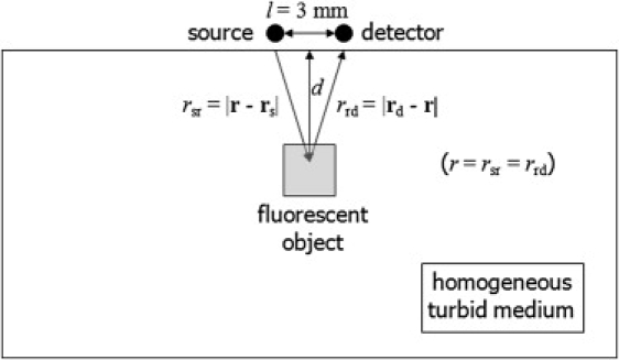
Schematic diagram of the experimental setup for the description of the photon migration.

Effect of parameters on the fluorescence TPSF

Fig. 3 A depicts the simulated fluorescence TPSFs when τ = 1 ns as a function of depth (d = 2, 4, 6, 8, 10 mm) to investigate the effect of depth on the fluorescence TPSF. The exponential time decay of the fluorescence TPSF, the so-called effective lifetime τ_eff (12,21), is evaluated by fitting it with a mono-exponential function from 80% peak intensity to 20% peak intensity, which ensures fitting to data with a good signal/noise ratio. The temporal position of the fluorescence TPSF maximum t_max increases with depth d, as clearly shown in Fig. 3 A. Fig. 3 B depicts the simulated fluorescence TPSFs when d = 2 mm as a function of lifetime (τ = 1, 2, 3, 4, 5 ns) to investigate the effect of lifetime τ on the fluorescence TPSF. As τ increases, the maximum value of the fluorescence TPSF decreases but it also broadens, so that each fluorescence TPSF results in the same CW intensity when it is integrated over t = 0 to infinity. The values τ_eff and t_max increase with τ, as clearly shown in Fig. 3 B.

Figure 3.

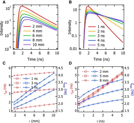
Fluorescence TPSFs as a function of (A) depth d and (B) lifetime τ of a fluorescence inclusion. The values τ_eff and t_max are plotted as a function of (C) r and (D) τ.

The values τ_eff and t_max can be expressed as functions of τ and d, and their relationship is shown in Fig. 3, C and D. We use (r_sr + r_rd) instead of d to get a clearer idea of the relationship between the pathlength of photon migration and (τ_eff, t_max). In addition, (r_sr + r_rd) can be expressed as 2r using the symmetry of the usual experimental device setup (as shown in Fig. 2), and thus, the depth d is easily calculated from r using $d=\sqrt{r^2-{\left(l/2\right)}^2}\text{.}$ In Fig. 3 C, τ_eff (red dashed lines with markers) and t_max (blue solid lines with markers) are plotted as a function of r at τ = 1, 3, 5 ns. As seen in Fig. 3 C, τ_eff and t_max have linear relationships with r for each lifetime value. From Fig. 3 C, r dependence of τ_eff and t_max leads us to confirm that t_max is a more sensitive parameter than τ_eff in estimating the depth of a fluorescence inclusion. In Fig. 3 D, τ_eff and t_max are plotted as a function of τ at d = 2, 5, and 8 mm. Unlike both the linear dependence of τ_eff and t_max on r, τ_eff is linear with τ, whereas t_max has a square-root relationship with $\tau \left(t_{\text{max}}\sim \sqrt{\tau }\right)$ at each depth (as shown in Fig. 3 D).

Approach to the relationship between intrinsic fluorophore properties and fluorescence TPSF measurements

CW fluorescence intensity, I_CW, is a good measure of the concentration of a fluorescent inclusion, if its depth-dependence is considered. Qualitatively, τ_eff is representative of τ. The value τ_eff ≅ τ, when a fluorescent inclusion is inscribed shallowly in a turbid medium or when τ is much larger than diffusion time. However, for a deep inclusion with nanosecond lifetime in a turbid medium, the values of τ and τ_eff have a quantitative difference—because of the convolution of exponential decay with the Green's function, which has a dependence on the location of a fluorescent inclusion. The value t_max gives the statistical description of the most probable time-of-flight of photons and this provides the information on the pathlength, i.e., depth. In this sense, I_CW, τ_eff, and t_max are said to be functions of n, τ, and d and vice versa; i.e., if (I_CW, τ_eff, t_max) = h(n, τ, d) is established, (n, τ, d) = h⁻¹(I_CW, τ_eff, t_max) can be determined. In terms of geometry, three surfaces determine one point which is the only real solution (n, τ, d) to the algebraic equation, given the easily measurable quantity (I_CW, τ_eff, t_max) in the three-dimensional parameter space.

CW intensity I_CW versus relative concentration n_rel

Intensity I(r) resulting from a fluorescence inclusion at position r can be obtained by integrating Green's function over t from 0 to ∞ (22),

$$I\left(r\right)=\left(\frac{1}{4\pi Dv}\right)\frac{e^{-{\mathit{\mu }}_{\text{eff}}r}}{r},{\mathit{\mu }}_{\text{eff}}=\sqrt{\frac{{\mathit{\mu }}_{\text{a}}}{D}}=\sqrt{3{\mathit{\mu }}_{\text{a}}\left({\mathit{\mu }}_{\text{a}}+{{\mathit{\mu }}^{\prime }}_{\text{s}}\right)},$$ (4)

where v is the speed of light in the medium, $D=1/3{\mu }_{\text{a}}+{{\mu }^{\prime }}_{\text{s}}$ is the diffusion constant related to the optical absorption, and ${\mathit{\mu }}_{\text{eff}}=\sqrt{\frac{{\mathit{\mu }}_{\text{a}}}{D}}=\sqrt{3{\mathit{\mu }}_{\text{a}}\left({\mathit{\mu }}_{\text{a}}+{{\mathit{\mu }}^{\prime }}_{\text{s}}\right)}$ is the effective attenuation coefficient. Here, $r=\sqrt{d^2+{\left(l/\text{2}\right)}^2},$ and l is the separation between source and detector, as shown in Fig. 2. Thus, the relationship between CW intensity, I_CW, and relative concentration, n_rel, is obtained as

$$I_{\text{CW}}\left(\mathbf{r}\right)=N\times \left(\frac{e^{-{\mathit{\mu }}_{\text{eff}}r}}{4\pi Dvr}\right)\times n\left(\mathbf{r}\right)\times \left(\frac{e^{-{\mathit{\mu }}_{\text{eff}}r}}{4\pi Dvr}\right)=n_{\text{rel}}\left(\mathbf{r}\right)\frac{e^{-2{\mathit{\mu }}_{\text{eff}}r}}{r^2}\text{.}$$ (5)

Because we do not recover the absolute fluorophore concentration, we use the term of relative concentration in arbitrary units to describe the fluorophore concentration. This is still useful when comparing the relative concentration of fluorophores for imaging studies. Fitting the simulated I_CW to Eq. 5 gives us μ_eff = 0.074 ± 0.0228 mm⁻¹, as shown in Fig. 4 A. Error bars of all the parameters were negligibly small, and R² = 0.998. Fitted μ_eff value is in quantitative agreement with the calculated value of μ_eff = 0.079 mm⁻¹ for μ_a = 2.0 × 10⁻³ mm⁻¹ and μ′_s = 1.05 mm⁻¹.

Figure 4.

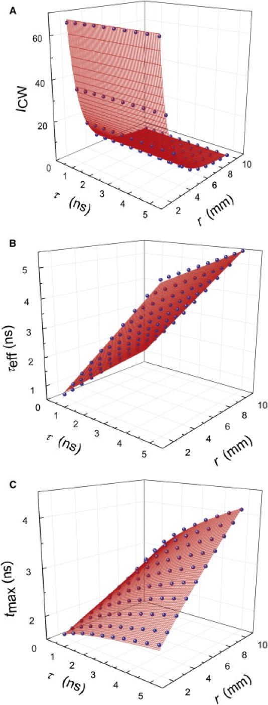
Three-dimensional scatter plots (blue circles) of (A) I_CW, (B) τ_eff, and (C) t_max of a fluorescence inclusion as a function of τ and r. Each surface plot (red lines) represents the third-dimensional fitting result.

Effective lifetime τ_eff versus lifetime τ

The value τ_eff is expected to increase with the pathlength 2r, as τ_eff is defined in terms of average decay time of the fluorescence TPSF. The differential pathlength factor (DPF) is defined in Hiraoka et al. (23), and here describes the photon propagation distance between the source or detector and the fluorophore, i.e., the differential pathlength (DP) defined in Wang and Wu (24), divided by the geometrical distance r, between the source or detector and the fluorophore. Therefore, τ_eff can be approximated as

$${\tau }_{\text{eff}}=a_1\left(\lambda \right)+\tau +\left(\frac{2\times \text{DPF}\left(\lambda \right)}{v}\right)r,$$ (6)

where a₁(λ) is a constant related with a system setup and the third term on the right-hand side represents the elongated lifetime (2r/v × DPF(λ)), due to the scattering through the path, and thus, it depends on the location of the fluorophore. Pathlength factor DPF(λ) for an infinite medium is given by (24)

$$\text{DPF}\left(\lambda \right)=\frac{1}{2}\frac{r\left(1+3{\mathit{\mu }}_{\text{a}}\left(\lambda \right)D\left(\lambda \right)\right)}{D\left(\lambda \right)+\sqrt{{\mathit{\mu }}_{\text{a}}\left(\lambda \right)D\left(\lambda \right)}\times r}\text{.}$$ (7)

For the values used here, the third term in Eq. 6 is not negligible and needs to be included. As τ_eff has a linear relationship with both τ and r, and there is no correlation between τ and r, the relationship can be explored by fitting the three-dimensional array of τ_eff to a linear function τ_eff = a₁ + b₁·τ + c₁·r. Three-dimensional surface scatter plot in Fig. 4 B shows that τ_eff can be expressed as a plane function of variables τ and r with a₁(λ) = 0.20 ± 0.016 ns, b₁(λ) = 1 (fixed), and c₁(λ) = 0.04 ± 0.003 ns/mm. The error bars of all the coefficients were negligibly small, and R² = 0.999. As DPF = 5.8 and $c_1\left(\lambda \right)\cong 2\times \text{DPF}\left(\lambda \right)/v=0.05\text{ns/nm}$ at λ = 760 nm (from Eq. 7) and v = 214.29 mm/ns (assuming the index of refraction to be 1.4), Eq. 6 is said to give a valid description of τ_eff. This approach is verified for a range of optical properties, μ_a = 1 × 10⁻⁴–1 × 10⁻² mm⁻¹ and μ′_s = 0.5–1.5 mm⁻¹.

Temporal position of the fluorescence TPSF maximum t_max versus depth d

The value t_max can be calculated by differentiating Eq. 3 with respect to t. For the simplicity of the analytic calculation, Eq. 3 can be rewritten as (3)

$$\begin{array}{c}{\varphi }_{\text{fl}}\left({\mathbf{r}}_s,{\mathbf{r}}_{\text{d}},t\right)=\mathit{\alpha }\underset{0}{\overset{t}{\int }}d{t}_{\text{E}}\frac{r_{\text{sr}}+r_{\text{rd}}}{r_{\text{sr}}{r}_{\text{rd}}}\frac{1}{{\left[4\pi Dv\left(t-t_{\text{E}}\right)\right]}^{3/2}}\\ \times \exp \left[-\frac{{\left(r_{\text{sr}}+r_{\text{rd}}\right)}^2}{4Dv\left(t-t_{\text{E}}\right)}\right]\exp \left[-{\mathit{\mu }}_{\text{a}}v\left(t-t_{\text{E}}\right)\right]\\ \times \frac{\exp \left(-t_{\text{E}}/\tau \right)}{\tau }.\end{array}$$ (8)

and t_max can be expressed as the following simple equation by calculating (dϕ_fl/dt) = 0 at t = t_max (25),

$$t_{\text{max}}=a_2\left(\lambda \right)+\frac{r\sqrt{\tau }}{\sqrt{Dv}},$$ (9)

where a₂(λ) is a constant related with a system setup. Equation 9 is in good agreement with the behavior of t_max curved plane as shown in Fig. 3, C and D. Thus, the relationship can be explored by fitting the three-dimensional array of t_max to a curved plane function $t_{\text{max}}=a_2+b_2·r\sqrt{\tau }$. The three-dimensional surface scatter plot in Fig. 4 C shows that t_max can be expressed as a curved plane function of variables τ and r with a₂(λ) = 1.578 ± 0.0125 ns, and b₂(λ) = 0.120 ± 0.0012 ns^1/2/mm. The error bars of all the coefficients were negligibly small, and R₂ = 0.990. Because $b_2\left(\lambda \right)\cong 1/\sqrt{Dv}=0.121$ ns^1/2/mm (D = 0.317 mm), Eq. 9 is said to give a valid description of t_max.

Novel algorithm

First, we can obtain a relationship between I_CW and n_rel via d using Eq. 5,

$$n_{\text{rel}}=I_{\text{CW}}\times r^2\times e^{2{\mathit{\mu }}_{\text{eff}}r}=I_{\text{CW}}\times \left[d^2+{\left(\frac{l}{2}\right)}^2\right]\times e^{2{\mathit{\mu }}_{\text{eff}}\sqrt{d^2+{\left(\frac{l}{2}\right)}^2}}\text{.}$$ (10)

Also, τ and r, i.e., $d=\sqrt{r^2-{\left(1/2\right)}^2},$ is expressed as analytical functions of measured τ_eff and t_max from the use of Eqs. 6 and 9, and a cubic equation (26),

$$\tau =4p\times {\cos }^2\left[\frac{1}{3}{\cos }^{-1}\left(-\sqrt{\frac{q^2}{p^3}}\right)\right],$$ (11)

$$r=\frac{\left(qv/\text{DPF}\right)}{2\sqrt{p}\times \cos \left[\frac{1}{3}{\cos }^{-1}\left(-\sqrt{\frac{q^2}{p^3}}\right)\right]},$$ (12)

where

$$p=\frac{{\tau }_{\text{eff}}-a_1}{3},q=\text{DPF}\sqrt{\frac{D}{v}}\left(t_{\text{max}}-a_2\right)\text{.}$$ (13)

That is, the relative concentration n_rel, lifetime τ, and the depth of a fluorescent inclusion d can be calculated analytically from the simple measurements of CW intensity I_CW, effective lifetime τ_eff, and the temporal position of the fluorescence TPSF maximum t_max using Eqs. 10–13. As discussed earlier, we assumed a priori background optical properties. However, errors in these a priori estimates in vivo would induce the errors in reconstructing n, τ, and d of the fluorophore as previously discussed in our recent work (21). To prove the robustness of the algorithm, we used a forward model to generate the fluorescence TPSFs for background optical properties with 10% changes in μ_a and μ′_s from the initial values of μ_a = 2 × 10⁻³ mm⁻¹ and μ′_s = 1.05 mm⁻¹ with τ = 1 ns and d = 5 mm. We found that Δμ_a = ±10% and Δμ′_s = ±10% induce such errors as Δn = ±18%, Δτ = ±9.2%, and Δd = 4.2% when μ_a and μ′_s are fixed to original values, which are reasonable errors given that the background optical properties can be estimated a priori within 10%. Admittedly, here we use the simple case of homogenous background optical properties as others have done (18), which in practice is an approximation to the inhomogeneous situation of a small animal and will introduce errors that are not assessed here. A priori knowledge of these background optical properties is assumed known from the published values (27), or from prior measurements of the small animal.

Cubic equation

Equations 6 and 9, when we set x ≅ τ and y ≅ r, and define the constant $A\equiv 2\times \text{DPF}\left(\lambda \right)/v,$ then become the problem of solving simultaneous equations,

$$x+Ay=3p,\sqrt{x}\times y=\frac{2q}{A},$$ (14)

which becomes the cubic equation for u,

$$u^3-3p\times u+2q=0,u\equiv \sqrt{x}>0.$$ (15)

As the discriminant of the cubic equation with this form D = (–p)³ + q² < 0 for given p and q in Eq. 13, the solution to Eq. 15 has three, distinct, real roots (26), which are given by

$$y_{\text{n}}=2\sqrt{p}\times \cos \left(\mathit{\varphi }+\frac{2\pi }{3}n\right)\left(n=0,1,2\right),$$ (16)

where ϕ is given by

$$\mathit{\varphi }=\frac{1}{3}{\cos }^{-1}\left(-\sqrt{\frac{q^2}{p^3}}\right)\text{.}$$ (17)

Of these three roots, the only physically reasonable solution to Eq. 14 is the largest value of these three roots (the other roots have x ≅ 0), and therefore, τ and $d=\sqrt{r^2-{\left(l/2\right)}^2}$ are given by Eqs. 11–13.

Results and Discussion

In vitro phantom study

Now we turn our attention to image reconstruction using the algorithm above. Fig. 1, A and B, shows scanning geometry. It is composed of a source and a detector, with 3-mm fixed separation, which are scanned in tandem in a 2-mm step. The diameter and the thickness of this cylindrical phantom were 15 mm and 8 mm, respectively. The imaged area is 3 × 3 cm². We analyze the 10 μM Cy7 phantom that was embedded in the Intralipid-1% medium with 99% water. The optical properties are μ_a = 2.0 × 10⁻³ mm⁻¹ and μ′_s = 1.05 mm⁻¹ at λ = 760 nm. Fig. 5, A, D, and G, shows the reconstruction maps of concentration n_num, lifetime τ_num, and depth d_num, respectively, for a pellet embedded at depth d_top = 5 mm (top surface of the medium to that of the fluorescent inclusion) using the deconvolution algorithm previously described in our previous work (21). Fig. 5, B, E, and H, shows the maps of CW Intensity I_CW, effective lifetime τ_eff, and the temporal position of the fluorescence TPSF maximum t_max, respectively, for the same pellet from the direct measurements of the fluorescence TPSF. Fig. 5, C, F, and I, shows the reconstruction maps of n_rel, τ_ana, and d_ana, respectively, using the new algorithm described in analytic Eqs. 10–13. Processing time in the evaluations of n_num, τ_num, and d_num maps for 16 × 16 pixels took ∼2.5 h using an inversion technique (21) in which we applied the Levenberg-Marquardt algorithm (28,29). However, it takes <15 s in reconstructing n_rel, τ_ana, and d_ana maps for the same pixel size using the algorithms introduced here, including the evaluations of I_CW, τ_eff, and t_max from the direct analysis of the fluorescence TPSF performed on an Intel Pentium 4, 3.06 GHz CPU. The Savitzky-Golay algorithm (30,31) has been used in smoothing the measured fluorescence TPSFs to remove high-frequency noise for the proper evaluations of I_CW, τ_eff, and t_max because the signal is relatively noisy deep inside the medium. Fig. 5, A–C, shows the reconstruction maps for n_num, I_CW, and n_rel. They provide nearly identical images in size and shape, and are very similar to the real size of the pellet (15-mm diameter) in Fig. 1, A and B. Fig. 5, D–F, shows the reconstruction maps for τ_num, τ_eff, and τ_ana. The τ_num and τ_ana maps also look identical in size and shape in Fig. 5, D and F, whose results from the different algorithms, nearly provide identical absolute values. This confirms the validity and superiority of the new algorithm in achieving equivalent results in significantly less time. From the conversion Eqs. 11–13, τ = 1 ns and d = 5 mm corresponds to τ_eff = 1.5 ns, which is clearly shown in Fig. 5 E and is also depicted as the simulated contour plot in our recent work (12). Fig. 5, G–I, shows the reconstruction maps for d_num, t_max, and d_ana. They also look identical in size and shape except for the differences in the values of d_num and t_max. The d_num and d_ana maps in Fig. 5, G and I, in particular, provide nearly identical values. From Eqs. 11–13, τ = 1 ns and d = 5 mm corresponds to t_max = 2.2 ns, which is clearly shown in Fig. 5 H and is also depicted as the simulated contour plot in our recent work (12).

Figure 5.

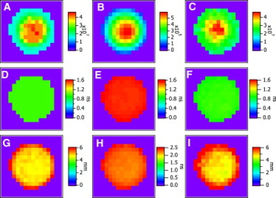
Image plots of a Cy7 inclusion for (A) n_num, (B) I_CW, (C) n_rel, (D) τ_num, (E) τ_eff, (F) τ_ana, (G) d_num, (H) t_max, and (I) d_ana.

In vivo mouse imaging

Now this algorithm is applied to in vivo mouse experiment. Cy7 10 μM was tail-vein injected in an anesthetized mouse. As expected, fluorescence signals are found in the bladder due to clearance and some accumulation in the liver (although this was not fully scanned). The optical properties of the mouse tissue were taken from the uniform mouse torso optical properties (μ_a = 0.002 mm⁻¹ and μ′_s = 1.26 mm⁻¹) (27). This corresponds to a DPF value of ∼5 from Eq. 7. Image reconstructions were conducted for these optical property values. Similar to the in vitro results, equivalent images were recovered from both the numerical and analytical methods for relative concentration, lifetime, and depth in vivo. As such, only the analytical images are presented for succinctness. Fig. 6 A depicts the mouse image with I_CW map at 12 min postinjection. Strong fluorescence signal (∼5 × 10⁵ counts) is found around the bladder, with less fluorescence signal (∼2 × 10⁵ counts) found around the liver. In the relative concentration map, Fig. 6 B, the ratio of signal in the center of the bladder to that at the edge of the liver, is larger than the I_CW map in Fig. 6 A and the signal from the liver is barely seen in Fig. 6 B. This is due to the shallower depth of the liver than the bladder, and compensation due to the rapid decay $\left(\sim e^{-2{\mu }_{\text{eff}}r}/r^2\right)$ of the CW intensity over depth, as described in Eq. 5. A reconstructed lifetime map is shown in Fig. 6 C in which only nonnegligible concentrations are shown. The value τ ≅ 0.4 ns is evaluated around the center of the bladder, and this is expected from direct measurement of the liquid Cy7. Fig. 6 D shows the depth map, in which only nonnegligible concentrations are shown, and is roughly d_bladder ≅ 4 mm—which is in good agreement with the estimated depth of bladder of the mouse (32,33). Fig. 6 E shows the fluorescence TPSF of bladder, edge of liver, and tissue, and the values for each of τ_eff and t_max. Maps of relative concentration, lifetime, and depth are calculated using the values of I_CW, τ_eff, and t_max at each pixel.

Figure 6.

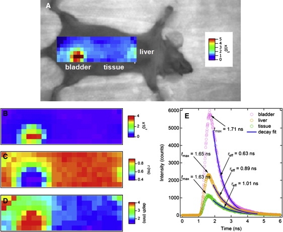
In vivo mouse imaging. (A) CW intensity (I_CW) map overlaid on a bright-field image. (B) Relative concentration (n_rel) map. (C) Lifetime (τ_ana) map. (D) Depth (d_ana) map. (E) At bladder, τ_eff = 0.63 ns and t_max = 1.71 ns correspond to τ = 0.40 ns and d = 4.0 mm using the new algorithm. At the edge of liver, τ_eff = 0.89 ns and t_max = 1.65 ns correspond to τ = 0.74 ns and d = 2.2 mm. At tissue, τ_eff = 1.01 ns and t_max = 1.63 ns correspond to τ = 0.88 ns and d = 1.7 mm.

Conclusions

We established an analytic method for the estimation of relative concentration, lifetime, and depth of a localized fluorescent object. They are derived from the simple measurements of I_CW, τ_eff, and t_max by analyzing the fluorescence TPSF. Due to the analytical nature of this algorithm, the time spent in the reconstruction of a few hundred pixels is reduced by three orders of magnitude. This algorithm is confirmed by phantom analysis. In addition, we showed that we can extend this method to in vivo study.

References

- 1.Bambot S.B., Lakowicz J.R., Rao G. Potential applications of lifetime-based, phase-modulation fluorimetry in bioprocess and clinical monitoring. Trends Biotechnol. 1995;13:106–115. doi: 10.1016/S0167-7799(00)88915-5. [DOI] [PMC free article] [PubMed] [Google Scholar]
- 2.Lakowicz J.R. 3rd Ed. Springer; New York: 2006. Principles of Fluorescence Spectroscopy. [Google Scholar]
- 3.Hall D.J., Ma G., Wang Y. Simple time-domain optical method for estimating the depth and concentration of a fluorescent inclusion in a turbid medium. Opt. Lett. 2004;29:2258–2260. doi: 10.1364/ol.29.002258. [DOI] [PubMed] [Google Scholar]
- 4.Graves E.E., Ripoll J., Ntziachristos V. A submillimeter resolution fluorescence molecular imaging system for small animal imaging. Med. Phys. 2003;30:7426–7431. doi: 10.1118/1.1568977. [DOI] [PubMed] [Google Scholar]
- 5.Hall D.J., Han S.-H. Preliminary results from a multi-wavelength time domain optical molecular imaging system. Proc. SPIE. 2007;6430:64300T. [Google Scholar]
- 6.Cole M.J., Siegel J., Wilson T. Whole-field optically sectioned fluorescence lifetime imaging. Opt. Lett. 2000;25:9885–9890. doi: 10.1364/ol.25.001361. [DOI] [PubMed] [Google Scholar]
- 7.Grant D.M., Elson D.S., Courtney P. Optically sectioned fluorescence lifetime imaging using a Nipkow disk microscope and a tunable ultrafast continuum excitation source. Opt. Lett. 2005;30:3353–3355. doi: 10.1364/ol.30.003353. [DOI] [PubMed] [Google Scholar]
- 8.Hall D.J., Sunar U., Han S.H. In vivo simultaneous monitoring of two fluorophores with lifetime contrast using a full-field time domain system. Appl. Opt. 2009;48:D74–D78. doi: 10.1364/ao.48.000d74. [DOI] [PubMed] [Google Scholar]
- 9.Kumar A.T.N., Skoch J., Dunn A.K. Fluorescence-lifetime-based tomography for turbid media. Opt. Lett. 2005;30:3347–3349. doi: 10.1364/ol.30.003347. [DOI] [PubMed] [Google Scholar]
- 10.Kumar A.T.N., Raymond S.B., Bacskai B.J. Time resolved fluorescence tomography of turbid media based on lifetime contrast. Opt. Express. 2006;14:12255–12270. doi: 10.1364/oe.14.012255. [DOI] [PMC free article] [PubMed] [Google Scholar]
- 11.Laidevant A., Da Silva A., Boccara A.C. Analytical method for localizing a fluorescent inclusion in a turbid medium. Appl. Opt. 2007;46:2131–2137. doi: 10.1364/ao.46.002131. [DOI] [PubMed] [Google Scholar]
- 12.Han S.-H., Hall D.J. Estimating the depth and lifetime of a fluorescent inclusion in a turbid medium using a simple time-domain optical method. Opt. Lett. 2008;33:1035–1037. doi: 10.1364/ol.33.001035. [DOI] [PubMed] [Google Scholar]
- 13.Hall D.J., Vera D.R., Mattrey R.F. Full-field time domain optical molecular imaging system. Proc. SPIE. 2005;5693:330–335. [Google Scholar]
- 14.Firbank M., Oda M., Delpy D.T. An improved design for a stable and reproducible phantom material for use in near-infrared spectroscopy and imaging. Phys. Med. Biol. 1995;40:955–961. doi: 10.1088/0031-9155/40/5/016. [DOI] [PubMed] [Google Scholar]
- 15.van Staveren H.J., Moes C.J.M., van Gemert M.J.C. Light scattering in Intralipid-10% in the wavelength range of 400–1100 nm. Appl. Opt. 1991;30:4507–4514. doi: 10.1364/AO.30.004507. [DOI] [PubMed] [Google Scholar]
- 16.Patterson M.S., Chance B., Wilson B.C. Time resolved reflectance and transmittance for the noninvasive measurement of tissue optical properties. Appl. Opt. 1989;28:2331–2336. doi: 10.1364/AO.28.002331. [DOI] [PubMed] [Google Scholar]
- 17.O'Leary M.A., Boas D.A., Yodh A.G. Fluorescence lifetime imaging in turbid media. Opt. Lett. 1996;21:158–160. doi: 10.1364/ol.21.000158. [DOI] [PubMed] [Google Scholar]
- 18.Ntziachristos V., Weissleder R. Experimental three-dimensional fluorescence reconstruction of diffuse media by use of a normalized Born approximation. Opt. Lett. 2001;26:893–895. doi: 10.1364/ol.26.000893. [DOI] [PubMed] [Google Scholar]
- 19.Li X.D., O'Leary M.A., Yodh A.G. Fluorescent diffuse photon density waves in homogeneous and heterogeneous turbid media: analytic solutions and applications. Appl. Opt. 1996;35:3746–3758. doi: 10.1364/AO.35.003746. [DOI] [PubMed] [Google Scholar]
- 20.Chandrasekhar S. Stochastic problems in physics and astronomy. Rev. Mod. Phys. 1943;15:1–89. [Google Scholar]
- 21.Han S.-H., Farshchi-Heydari S., Hall D.J. Analysis of the fluorescence temporal point-spread function in a turbid medium and its application to optical imaging. J. Biomed. Opt. 2008;13:064038. doi: 10.1117/1.3042271. [DOI] [PubMed] [Google Scholar]
- 22.Bassani M., Martelli F., Contini D. Independence of the diffusion coefficient from absorption: experimental and numerical evidence. Opt. Lett. 1997;22:853–855. doi: 10.1364/ol.22.000853. [DOI] [PubMed] [Google Scholar]
- 23.Hiraoka M., Firbank M., Delpy D.T. A Monte Carlo investigation of optical pathlength in inhomogeneous tissue and its application to near-infrared spectroscopy. Phys. Med. Biol. 1993;38:1859–1876. doi: 10.1088/0031-9155/38/12/011. [DOI] [PubMed] [Google Scholar]
- 24.Wang L.V., Wu H.-I. John Wiley; Hoboken, NJ: 2007. Biomedical Optics: Principles and Imaging. [Google Scholar]
- 25.Hall, D. J., G. Ma, …, P. Gallant. 2007. Time-domain method and apparatus for determining the depth and concentration of a fluorophore in a turbid medium. United States Patent Application Publication No. US2007/0158585 A1. (ART, Advanced Research Technologies Inc., Montreal, QC, Canada).
- 26.Nickalls R.W.D. A new approach to solving the cubic: Cardan's solution revealed. Math. Gaz. 1993;77:354–359. [Google Scholar]
- 27.Alexandrakis G., Rannou F.R., Chatziioannou A.F. Tomographic bioluminescence imaging by use of a combined optical-PET (OPET) system: a computer simulation feasibility study. Phys. Med. Biol. 2005;50:4225–4241. doi: 10.1088/0031-9155/50/17/021. [DOI] [PMC free article] [PubMed] [Google Scholar]
- 28.Levenberg K. A method for the solution of certain non-linear problems in least squares. Q. Appl. Math. 1944;2:164–168. [Google Scholar]
- 29.Marquardt D.W. An algorithm for least-squares estimation of nonlinear parameters. J. Soc. Ind. Appl. Math. 1963;11:431–441. [Google Scholar]
- 30.Savitzky A., Golay M.J.E. Smoothing and differentiation of data by simplified least squares procedures. Anal. Chem. 1964;36:1627–1639. [Google Scholar]
- 31.Steinier J., Termonia Y., Deltour J. Comments on smoothing and differentiation of data by simplified least square procedure. Anal. Chem. 1972;44:1906–1909. doi: 10.1021/ac60319a045. [DOI] [PubMed] [Google Scholar]
- 32.Chernomordik V., Hattery D., Gandjbakhche A.H. Inverse method of 3D reconstruction of localized in-vivo fluorescence. Application to Sjogren syndrome. IEEE J. Sel. Top. Quantum Electron. 1999;5:930–935. [Google Scholar]
- 33.D'Andrea C., Spinelli L., Cubeddu R. Localization and quantification of fluorescent inclusions embedded in a turbid medium. Phys. Med. Biol. 2005;50:2313–2327. doi: 10.1088/0031-9155/50/10/009. [DOI] [PubMed] [Google Scholar]