Detecting rare variants for complex traits using family and unrelated data

Abstract

Large genome-wide association studies have been performed to detect common genetic variants involved in common diseases, but most of the variants found this way account for only a small portion of the trait variance. Furthermore, candidate gene based resequencing suggests that many rare genetic variants contribute to the trait variance of common diseases. Here we propose two designs, sibpair and unrelated-case designs, to detect rare genetic variants in either a candidate gene based or genome-wide association analysis. First we show that we can detect and classify together rare risk haplotypes using a relatively small sample with either of these designs, and then have increased power to test association in a larger case-control sample. This method can also be applied to resequencing data. Next we apply the method to the Wellcome Trust Case Control Consortium (WTCCC) coronary artery disease and hypertension data, the latter being the only trait for which no genome-wide association evidence was reported in the original WTCCC study, and identify one interesting gene associated with hypertension and four associated with coronary artery disease at a genome-wide significance level of 5%. These results suggest that searching for rare genetic variants is feasible and can be fruitful in current genome-wide association studies, candidate gene studies or resequencing studies.

Introduction

When mapping genes contributing to common diseases, a popular hypothesis is the common disease common variants (CD-CV) assumption that the putative causal variants are common in the population at large and can express a sizable portion of the phenotypic variation.[Chakravarti 1999; Lander 1996; Reich and Lander 2001] An example that supports this assumption, the association of the APOE ε4 allele with Alzheimer disease and heart disease has long been known[Corder, et al. 1993]. The ε4 allele frequency ranges from 0.05 to 0.41 in different world populations[Fullerton, et al. 2000]. Under the CD-CV assumption, genetic variants underlying common diseases can be detected by testing a large number of tagging SNPs across the genome through linkage disequilibrium (LD) methods[Gabriel, et al. 2002; Risch and Merikangas 1996; Risch 2000]. Such theoretical and empirical evidence led to the launch of the International HapMap Project [2003; 2005; Frazer, et al. 2007], which focuses on understanding the pattern of common variants in the genome and their LD in four population samples. As an example, tagging SNPs can be selected for genotyping in order to improve efficiency and reduce cost. This also led to the technological advance of dense SNP genotyping, such as with Affymetrix and Illumina chips, with good coverage of the human genome attained by genotyping hundreds of thousands of SNPs at a time. As a result, we are able to study large and well-characterized clinical samples at affordable cost [2007]. This strategy recently led to the detection of many common susceptibility genetic variants responsible for complex diseases, such as rheumatoid arthritis[Plenge, et al. 2007; Thomson, et al. 2007], coronary artery disease (CAD)[McPherson, et al. 2007; Samani, et al. 2007] and type 2 diabetes[Saxena, et al. 2007; Zeggini, et al. 2007].

However, it has also been observed that the genetic variants identified through genome-wide association studies (GWAS) have accounted for only a small portion of the presumed genotypic variation, and hence many variants remain to be discovered [McCarthy, et al. 2008]. For example, human adult height has been a well-known heritable trait with heritability ranging around 0.81[Perola, et al. 2007]. Yet three recent GWAS of height [Gudbjartsson, et al. 2008; Lettre, et al. 2008; Weedon, et al. 2008], in a combined sample size of 63,000 individuals, identified a total of 54 independent variants influencing height, with each locus explaining ~0.3%-0.5% of the phenotypic variance[Visscher 2008]. Under the CD-CV assumption, the effect sizes of most of the common risk variants will be modest and require large sample sizes to detect them. Thus, we still face great challenges in order to uncover the rest of the genetic variants contributing to the variation of a complex trait. The CD-CV assumption has been heatedly debated, with the proposal of the alternative assumption of common disease-multiple rare variants (CD-MRV). Although family based linkage analysis has been considered less powerful than association analysis for identifying complex-disease genes [Risch 2000], lack of association evidence is found in the regions identified by linkage analysis. For example, linkage evidence has been consistently detected on chromosome 3q27 to obesity related traits in various populations [Kissebah, et al. 2000; Luke, et al. 2003; Zhu, et al. 2002] but no variant has been reported in GWAS in this region. It may be possible that multiple variants within a gene, either common or rare, contribute to the phenotypic variation, resulting in the lack of power in association studies.

Simulation studies have suggested that the frequency spectrum of causal variants is likely to be broad because of the collective effect of mutations, random genetic drift and selection, indicating that many disease susceptibility alleles could be relatively rare[Iyengar and Elston 2007; Pritchard 2001; Weiss and Terwilliger 2000]. For the past two decades the genetic basis of breast cancer has been intensively investigated and three classes of breast cancer susceptibility variants have been suggested: rare high-penetrance variants, rare moderate-penetrance variants and common low-penetrance variants[Stratton and Rahman 2008; Walsh and King 2007]. The genetic architecture of breast cancer may suggest that common diseases follow a similar pattern, with both rare and common variants contributing to the trait. In fact, studies of HDL cholesterol as a model trait have found that multiple rare genetic variants in the coding regions of regulatory genes, including ABCA1, APOA1, and LCAT, are significantly over-represented in the lower tail of the distribution[Cohen, et al. 2004; Frikke-Schmidt, et al. 2004]. Recently, population-based resequencing methods have uncovered rare genetic variants associated with metabolic phenotypes[Cohen, et al. 2005; Cohen, et al. 2006a; Cohen, et al. 2006b; Kotowski, et al. 2006; Romeo, et al. 2007] and plasma angiotensinogen level[Zhu, et al. 2005]. The current strategy used to search for rare variants is by sequencing candidate genes in the selected disease group. The frequencies of the identified rare variants are then compared to those in selected control groups. Variants are further assessed for their potential function in the relevant gene product, such as by their occurrence in conserved regions causing change in protein structure[Bodmer and Bonilla 2008; Cohen, et al. 2006a]. The challenges of such studies are the identification of candidate genes, the choice of appropriate cases, the need for deep DNA resequencing of many genes in a large number of individuals, and the assessment of the functional consequences of variants. This strategy has also led to the detection of mutations in three renal salt handling genes - SLC12A3, SLC12A1 and KCNJ1 - contributing to human blood pressure variation[Ji, et al. 2008].

When resequencing data are available and rare variants are reliably genotyped, the combined multivariate and collapsing (CMC) method can be a powerful method to detect rare variants that contribute to phenotypic variation provided the functional rare variants can be reasonably well classified [Li and Leal 2008]. Although resequencing technology is fast developing, it is still prohibitively expensive to conduct whole genome resequencing, or resequencing within genes for a large number of samples. When multiple rare loci contribute to a disease risk, current statistical methods, which consider each genetic marker or individual haplotype separately, lack statistical power and therefore require larger samples to detect the rare variants[Marchini, et al. 2004]. In addition, rare variants are not well tagged by the common SNPs available in the currently available chips [Bhangale, et al. 2008]. Thus, novel powerful statistical methods to detect rare variants under the current designs of GWAS are in great need for association studies.

Material and Methods

For the current GWAS in which the common SNPs are tagged, directly testing rare variants or collapsing rare variants is impossible because most of the rare variants are either not genotyped or not well called. It is then important to develop a method of testing rare variants without using the rare variants directly. Intuitively, we could use haplotypes consisting of a set of common SNPs to tag the rare variants we are interested in. Although the rare variants are usually not well tagged by common variants, it is reasonable to assume that one or more rare variants may fall on only one haplotype consisting of common SNPs. We can argue that a rare variant is introduced into a population later than common variants. When the frequency of a haplotype is small, we would expect a substantial fraction of the haplotypes to carry the rare variants (Figure 1). This is a reasonable assumption because most of the frequencies of haplotypes consisting of many SNPs will mostly be small, as demonstrated below in our application of the method to the WTCCC data in which 30 SNPs were analyzed at a time. Because the relative risks of rare variants are considered much larger than those of common risk variants, the average relative risk of a haplotype could still be relatively high, even if only a fraction of those with the haplotype carry the rare risk variants. Consider a particular haplotype H that consists of several genotyped SNPs. We denote by H_r and H_r̄ those individual haplotypes respectively carrying and not carrying the risk allele of an untyped rare variant. Then the probability of being diseased, given haplotype H, is $P(\mathit{disease}\mid H)=P(\mathit{disease}\mid H_{\overline{r}})(\frac{P(\mathit{disease}\mid H_r)P(H_r)}{P(\mathit{disease}\mid H_{\overline{r}})P(H)}+1\times \frac{P(H_{\overline{r}})}{P(H)})$. Thus, the relative risk of haplotype H is the average risk of haplotypes H carrying and not carrying the rare risk allele (this latter is 1) weighted by their frequencies. When the frequency of haplotype H is small in a population, we would expect a substantial fraction of the H haplotypes to carry the rare risk allele and, therefore, the relative risk of H may still be large. In the following discussion, we only consider a haplotype that may carry a rare risk allele. We call such a haplotype that carries at least one risk allele a risk haplotype. As we discussed above, we only need to adjust the relative risk of a haplotype if it carries untyped rare risk alleles only a fraction of the time. Rather than simply testing individual haplotypes or SNPs for association, our idea to detect rare variants includes two stages. We first identify a set of risk haplotypes using a small proportion of the sample and then test for association with that set of identified haplotypes in an association study. Because we test the set of rare risk haplotypes collectively, the cumulative frequency of such risk haplotypes can be large and hence the power can be substantially increased.

Figure 1.

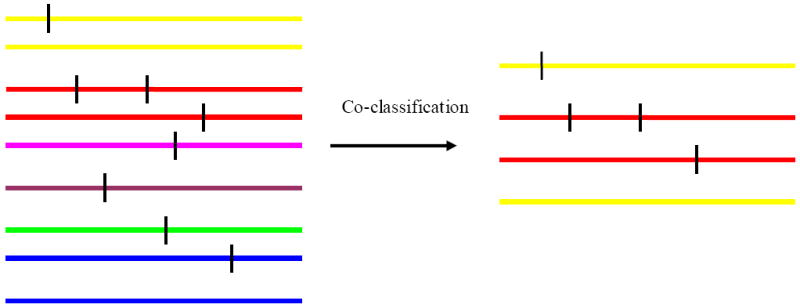
Hypothetical rare haplotypes and disease variants. Each colored line represents a haplotype created by genotyped markers. The vertical bars represent rare disease variants. The rare disease variants may not be genotyped. Lines with the same color represent the same haplotype as represented by genotyped markers. Co-classification can classify some haplotypes which carry rare disease variants into a group. But some haplotypes that do not carry any disease variants may also be mistakenly co-classified. However, most classified haplotypes carry disease variants.

Enrichment of rare risk haplotypes in cases

Assume we study haplotypes in a candidate gene or a small genomic region. We expect the risk haplotype frequencies to be enriched among cases. Let H = {H₁, H₂,. . H,_k} be a set of rare risk haplotypes with the corresponding haplotype frequencies h₁, h₂,…, h_k in affected cases and h₁⁰, h₂⁰,…, h_k⁰ in a general population, and let H_k+1 be the rest of the (non-risk) haplotypes with total frequency h_k+1 in cases and $h_{k+1}^0$ in controls, respectively. We also define the cumulative risk haplotype frequency $p=\sum _{i=1}^k{h}_i^0$. We can calculate the frequency of a rare risk haplotype H_i among cases as

$$\begin{array}{l}{h}_i=P(H_i\mid \mathit{affected})\\ =\frac{P(\mathit{affected}\mid H_i{H}_i)P(H_i{H}_i)+0.5\sum _{j\ne i}P(\mathit{affected}\mid H_i{H}_j)P(H_i{H}_j)+0.5P(\mathit{affected}\mid H_i{H}_{k+1})P(H_i{H}_{k+1})}{P(\mathit{affected})}.\end{array}$$

Thus, we can write h_i = ϕ(λ, p)h_i⁰, where $\phi (\lambda ,p)=\frac{\sqrt{\lambda }}{\sqrt{\lambda }p+1-p}$ for a multiplicative mode of inheritance; $\phi (\lambda ,p)=\frac{\lambda }{\lambda -{(1-p)}^2(\lambda -1)}$ for a dominant mode of inheritance; and $\phi (\lambda ,p)=\frac{p(\lambda -1)+1}{p^2(\lambda -1)+1}$ for a recessive mode of inheritance, respectively, where λ is the genotypic relative risk. (See Appendix A). The enrichment factor ϕ(λ, p) depends only on the genotypic relative risk λ and the cumulative risk haplotype frequency p. In figure 2, the top panel demonstrates the relationship between the enrichment factor ϕ(λ, p) and λ and p for the three modes of inheritance. It is apparent that ϕ(λ, p) is largest for a dominant mode, followed by a multiplicative mode. The enrichment factor for a recessive mode of inheritance is much smaller, and ϕ(λ, p) decreases as the cumulative risk haplotype p increases.

Figure 2.

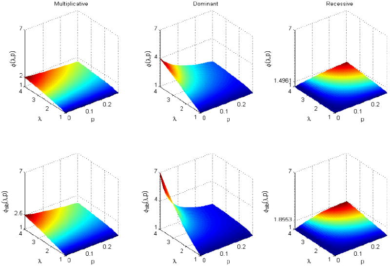
Plots of the enrichment factors ϕ(λ, p) and ϕ_sib(λ, p) against λ and p for multiplicative, dominant and recessive modes of inheritance. ϕ_sib(λ, p) is always larger than ϕ(λ, p). Both enrichment factors increase as λ increases, but decrease as p increases.

Enrichment of rare risk haplotypes in affected sibpairs

Since a risk variant segregates within families, rare risk haplotypes may be further enriched in affected sibpairs. We now demonstrate that rare risk haplotypes can be enriched in affected sibpairs. We use the same notation as above, except that we let h₁, h₂,…, h_k be the risk haplotype frequencies and h_k+1 be the rest of the (non-risk) haplotype frequency, respectively, in affected sibpairs. Let s₁ and s₂ be two sibs of a sibpair, where s_i = 1 if the i-th sib is affected and 0 if not affected. Then the frequency of a rare risk haplotype H_i in affected sibpairs can be written as (Appendix A) h_i = P(H_i ∣ s₁ = s₂ = 1) = ϕ_sib(λ, p)h_i⁰, where

1. Under a multiplicative model, f₂ = λf₀, $f_1=\sqrt{\lambda }{f}_0$,

   $${\phi }_{\mathit{sib}}(\lambda ,p)=\frac{\sqrt{\lambda }[{(\sqrt{\lambda }-1)}^3{p}^3+(2\sqrt{\lambda }+5){(\sqrt{\lambda }-1)}^2{p}^2+(\sqrt{\lambda }-1)(\lambda +3\sqrt{\lambda }+7)p+\sqrt{\lambda }+3]}{{[{(\sqrt{\lambda }p+1-p)}^2+\lambda p+1-p]}^2};$$
2. Under a dominant model, f₂ = f₁ = λ f₀,

   $${\phi }_{\mathit{sib}}(\lambda ,p)=\frac{\frac{1}{4}\lambda [3p(p-2)(1-\lambda )+3+\lambda ]}{\frac{1}{4}{[\lambda p(2-p)+{(1-p)}^2]}^2+\frac{1}{2}[{\lambda }^2{p}^2(3-2p)+\lambda (2+\lambda )p{(1-p)}^2+{(1-p)}^3]+\frac{1}{4}[{\lambda }^{2}p(2-p)+{(1-p)}^2]};$$
3. Under a recessive model, f₂ = λ f₀, f₁ = f₀,

   $${\phi }_{\mathit{sib}}(\lambda ,p)=\frac{1+\frac{1}{4}{(\lambda -1)}^2{p}^3+\frac{1}{4}(2\lambda +1)(\lambda -1)p^2+\frac{1}{4}(\lambda +4)(\lambda -1)p}{\frac{1}{4}{[\lambda p^2-p^2+1]}^2+\frac{1}{2}[1+{(\lambda -1)}^2{p}^3+2(\lambda -1)p^2)]+\frac{1}{4}[{\lambda }^2{p}^2-p^2+1]}.$$

Figure 2, bottom panel, demonstrates the relationship between the enrichment factor ϕ_sib(λ, p) and λ and p for different modes of inheritance. The enrichment factor ϕ_sib(λ, p) is larger than that in unrelated cases for each of the corresponding three modes of inheritance, although the general pattern is similar.

Stage 1. Co-classifying rare risk haplotypes using cases or affected sibpairs

We have seen that rare risk haplotypes can be enriched in cases or affected sibpairs. We first introduce a method to co-classify rare risk haplotype using unrelated cases, which we call an unrelated-case design, although controls are required. We co-classify the rare risk haplotypes by defining the rare risk haplotype set as $S=\left\{H_i\mid h_i-h_i^0>\mu \sqrt{\frac{h_i^0(1-h_i^0)}{2N}}\right\}$, where N is the number of cases used for co-classification and μ is a predefined constant. Since h_i⁰ is usually unknown in practice, we estimate it from the controls.

We can similarly define the rare risk haplotype set for affected sibpairs, which we call the affected sibpair design. In this case, we define the rare risk haplotype set by $S=\left\{H_i\mid h_i-h_i^0>\mu \sqrt{\frac{h_i^0(1-h_i^0)}{3N}}\right\}$, where N is the number of affected sibpairs, h_i is the frequency of rare risk haplotype H_i in affected sibpairs, and h_i⁰ and μ are defined as before. Here we used 3N because there are only 3N independent haplotypes in N sibpairs under the null hypothesis.

When the haplotype frequencies in a population are known, the theoretical power to co-classify a rare risk haplotype for the unrelated-case design is the probability of observing more than $\left[2N\left(h_i^0+\mu \sqrt{\frac{h_i^0(1-h_i^0)}{2N}}\right)\right]$ rare haplotype in 2N Bernoulli trials. Here [x] denotes the largest integer less than x. For N affected sibpairs, the theoretical power is the probability of observing more than $\left[3N\left(h_i^0+\mu \sqrt{\frac{h_i^0(1-h_i^0)}{3N}}\right)\right]$ rare haplotypes in 3N Bernoulli trials. Figure 3 shows the power to co-classify a rare risk haplotype with 300 affected sibpairs or 600 cases for genotypic relative risks in the range 1.2-3.0 for multiplicative, dominant and recessive modes of inheritance. We took the cumulative risk haplotype frequency be 10% and chose μ = 1.28. We examined the power to co-classify an individual with risk haplotype frequency 0.5% (Figure 3 left panel) and 1% (Figure 3 right panel), respectively. In general, we observed that the affected sibpair design has more power to co-classify rare risk haplotypes than the unrelated-case design when the number of individuals is the same. The power decreases as the individual risk haplotype frequency decreases. Power will also decrease when the cumulative risk haplotype frequency increases (data not shown).

Figure 3.

Theoretical power of co-classifying rare risk haplotypes for the sibpair and unrelated-case designs. Three modes of inheritance were considered: multiplicative f₂ = λ f₀, $f_1=\sqrt{\lambda }{f}_0$; dominant f₂ = f₁ =λ f₀ and recessive f₂ = λ f₀, f₁ = f₀. Haplotype frequencies in the population are known. 300 affected sibpairs and 600 unrelated cases were used. The cumulative risk haplotype frequency is 10%. Left panel: individual risk haplotype frequency is 0.5%. Right panel: individual risk haplotype frequency is 1.0%.

Stage 2. Association test

After we obtain the risk haplotype set S using an unrelated-case or affected sibpair design, we can detect association between the set S and a disease by comparing the frequency of haplotypes in S between cases and controls using Fisher’s exact test. When the haplotypes in S carry rare risk variants, we would expect a substantial difference in the cumulative haplotype frequencies between cases and controls, and would therefore expect good power. For comparison, we also performed single marker analysis by comparing the allele frequency between cases and controls. The minimum p-value for testing the set of markers was corrected by the estimated effective number of tests [Nyholt 2004].

Simulation results using ACE gene haplotype frequencies

We obtained the haplotype frequencies in the ACE gene from our previous hypertension study in African samples [Zhu, et al. 2001]. There were 13 polymorphisms genotyped in this gene, resulting in a total of 149 different haplotypes with frequencies≥0.01% (Supplementary Table 1). The allele frequency for each polymorphism and the LD pattern among the polymorphisms are presented in supplementary table 1. We set 8 rare haplotypes, with frequencies in the range 1.0%-1.5% and with a cumulative risk haplotype frequency of 10%, to be risk haplotypes. For illustration, we assumed their effect on the phenotype is the same, i.e. that penetrance is only dependent on how many risk haplotypes an individual carries. However, this is not a necessary assumption in our method. An individual’s genotype was simulated by randomly drawing two haplotypes according to the haplotype frequencies. Disease status was simulated based on the penetrance, given the haplotypes, according to the three modes of inheritance. To simulate affected sibpairs, we independently simulated two individuals as the parents and then randomly transmitted one of the two haplotypes for each parent to his/her offspring. We kept generating sib pairs from parent-pairs until we generated enough affected sibpairs.

We first simulated 1,900 cases and 3000 controls for the unrelated-case design so that the total sample size was approximately equivalent to that of the WTCCC study[2007]. To perform the two-stage analysis, we randomly selected 300 cases for the co-classification stage 1 and used the remaining 1600 cases for the stage 2 association test. Since the power of the association test is dependent on the risk haplotypes being identified at stage 1 and the sample size at stage 2, we also examined the power for 400, 600, 800 and 1000 cases respectively at stage 1 and the corresponding number of remaining cases at stage 2. We assumed that the haplotype frequencies in the population are unknown and 1,000 controls were used to estimate their frequencies. Thus, we always used 2,000 controls at the stage 2 association test. We made comparisons with the affected sibpair design by simulating 150, 200, 300, 400 and 500 affected sibpairs respectively at the co-classification stage 1, and the same sample sizes at the stage 2 association test as for the unrelated-case design. Thus, the total sample size at stages 1 and 2 together was equivalent for the unrelated case and affected sibpair designs. We used μ = 1.28 to co-classify rare risk haplotypes at stage 1.

Table 1 presents the type I error for the two-stage method for both the unrelated-case and affected sibpair designs. The type I error was calculated at stage 2 based on 1,000 replications when the genotypic relative risk was set to 1.0. We observed reasonable type I error rates for both designs.

Table 1.

Type I error for the unrelated-case (UC) and affected sibpair (AS) designs.

No of unrelated cases/No of sibpairs at stage 1	300/150		400/200		600/300		800/400		1000/500
Significance level	0.05	0.01	0.05	0.01	0.05	0.01	0.05	0.01	0.05	0.01
Phase known
UC	0.039	0.009	0.04	0.004	0.04	0.006	0.048	0.01	0.047	0.011
AS	0.047	0.02	0.046	0.012	0.044	0.01	0.055	0.009	0.048	0.009
Phase unknown
UC	0.053	0.009	0.053	0.014	0.052	0.008	0.049	0.007	0.046	0.012
AS	0.052	0.013	0.067	0.011	0.051	0.011	0.055	0.013	0.056	0.015

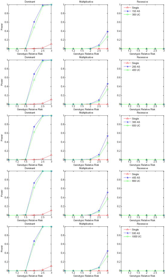
Figure 4 presents the power of the unrelated-case and affected sibpair designs for a variety of sample sizes at the co-classification stage 1 when haplotype phases are known, based on 1,000 replications. We estimated the power at the 10^-6 significance level, which can be considered as a genome-wide significance level of 0.05 after adjusting for 50,000 independent tests. When we perform one test in each gene, this number would be more than the maximum number of tests over the whole genome. We observed that the affected sibpair design is always more powerful than the unrelated-case design. When the haplotype phases are known, 800 cases or 400 affected sibpairs at stage 1 has the best power for the situations considered in our simulations, while 600 cases or 300 affected sibpairs result in similar power. For a dominant mode of inheritance there is apparently better power than for either multiplicative or recessive modes - in fact the recessive mode has virtually no power for either design. Both designs have over 80% power for a dominant mode for the various sample sizes at stage 1 when the genotypic relative risk is over 2.0. For comparison, we present the power of single SNP analysis, correcting for multiple tests using the method suggested by Nyholt[Nyholt 2004]. For the single SNP association test, we calculated power by comparing the allele frequencies between the 2,000 cases and 3,000 controls. There is almost no power for single SNP analysis after correcting for multiple comparisons. We further examined whether linkage analysis will have power to detect the linkage evidence when multiple rare risk haplotypes contribute to phenotypic variation by using the samples at stage 1 of the affected sibpair design. We present the linkage evidence by calculating the mean test Z score of alleles shared IBD for a variety of numbers of affected sibpairs. We observed that linkage analysis can have reasonable power when there are multiple rare risk haplotypes affecting the phenotype. This simulation also demonstrates that single SNP association analysis can easily miss underlying rare genetic variants - even when the linkage analysis suggests evidence of a susceptibility variant.

Figure 4.

Power comparison for the affected sibpair design, unrelated-case design and single marker analysis. Power was calculated at the 10^-6 significance level based on 1,000 replications. Haplotype phases are known. Haplotype frequencies were based on the ACE gene in an African population. There are 8 true risk haplotypes and the corresponding haplotype frequencies are between 1.0%-1.5% with cumulative risk haplotype frequency 10%. The lines represent the power of the three different modes of inheritance for different sample sizes used at stage 1, with the total sample size always kept the same. Single SNP association analysis was conducted on 2000 cases and 3000 controls but corrected for multiple comparisons[Nyholt 2004]. Linkage score was averaged from 1,000 replications using the mean test score of alleles shared identical by descent.

The above analysis is based on known haplotype phase, which will be unlikely in practice. We thus performed the analysis by pretending that haplotype phase was unknown and was inferred, using PHASE [Stephens, et al. 2001] for unrelated individuals and Merlin [Abecasis, et al. 2002] for sibpairs. Figure 5 presents the power of the same simulation data as in Figure 4 but with the haplotype phase inferred. As expected, the power of detecting association is less than when we know the haplotype phase. However, we still obtain reasonably good power for a dominant mode of inheritance when the genotypic relative risk is over 2.0. The power of the affected sibpair design is still much better than that of the unrelated-case design. For the unrelated-case design, 600 or 800 cases at stage 1 has the best power for the situations considered in our simulations, which is similar to that when haplotype phase is known. Similarly, 300 or 400 affected sibpairs has the best power among the variety of sample sizes at stage 1. We examined the percentage of the number of true risk haplotypes co-classified for the different sample sizes at stage 1 for both designs (Supplementary Table 2). We observed that the distribution of the number of true risk haplotypes co-classified approaches the true number of rare risk haplotypes as the sample size increases. However, this approach is not as fast as that found when the genotypic relative risk increases.

Figure 5.

Power comparison for the affected sibpair design, unrelated-case design and single marker analysis. Power was calculated at the 10^-6 significance level based on 1,000 replications. Haplotype phases are unknown and were inferred by PHASE. Haplotype frequencies were based on the ACE gene in an African population. There are 8 true risk haplotypes and the corresponding haplotype frequencies are between 1.0%-1.5% with cumulative risk haplotype frequency 10%. The lines represent the power of the three different modes of inheritance for different sample sizes used at stage 1, with the total sample size always kept the same. Single SNP association analysis was conducted on 2000 cases and 3000 controls but corrected for multiple comparisons[Nyholt 2004]. Linkage score was averaged from 1,000 replications using the mean test score of alleles shared identical by descent.

We next examined the power performance when less frequent risk haplotypes contribute to disease. To do this, we set 15 rare haplotypes, with frequencies in the range 0.56%-1.0% and with a cumulative risk haplotype frequency of 10%, to be risk haplotypes. We observed that the power was slightly less than that when the risk haplotype frequency is relatively high, although the power pattern is similar (Supplementary Figures 1 (phase known) and 2 (phase unknown)). Similarly, we observed 800 cases or 400 affected sibpairs at stage 1 has the best power for the situations considered in our simulations, while 600 cases or 300 affected sibpairs have similar power. We further reduced the cumulative risk haplotype frequency to 3.3% by setting only 4 of the 15 haplotypes as risk haplotypes. In this case we observed that 400 cases or 200 affected sibpairs at stage 1 has the best power (Supplementary Figure 3), suggesting it would be better to put more samples in the stage 2 association analysis when the cumulative risk haplotype frequency is low.

Application to the WTCCC hypertension and coronary artery disease data

The whole genome association study performed by the WTCCC studied seven major diseases in the British population. Many new genetic variants were detected to be associated with these diseases, but only one was detected for coronary artery disease (CAD) and none for hypertension (HT), which appears to offer a challenge. We reasoned that many rare genetic variants may contribute to the variation of these two diseases, and so applied our method to the WTCCC HT and CAD data. We downloaded the genotype data called by the algorithm CHIAMO for the HT and CAD samples and the shared controls (which consist of the 1958 Birth Cohort (58C) and UK Blood Service sample (NBS)) from the WTCCC website. The individuals dropped in the WTCCC study were also excluded in our analysis, resulting in 1952 HT cases, 1926 CAD cases and 2838 controls. We applied the same criteria as the WTCCC study for SNP exclusion, except that we kept all the SNPs with minor allele frequencies<1%. These criteria include: 1) missing genotype proportion >1%; 2) HWE exact test p-value < 5.7×10^-7 in controls; 3) allele frequency difference test based on 1df Trend Test p-value < 5.7×10^-7 or genotype frequency difference based on 2df General Test <5.7×10^-7 between 58C and NBS. After the QC analysis, 405,401 and 408,084 SNPs remained for the analysis for HT and CAD, respectively.

We first mapped a SNP to a particular gene if the SNP is within, or close to, the gene. If a SNP is located between two neighboring genes, we mapped it to the gene that has the closer physical distance to it. We used the map created by Wang et al. [Wang, et al. 2007] as a reference. Haplotypes were inferred using the software fastPHASE, [Scheet and Stephens 2006] which minimizes the switch error in every gene. When the number of SNPs within a gene was greater than 30, the analysis was performed on every sequence of 30 consecutive SNPs. Since we do not know the cumulative risk haplotype frequency for these two diseases, we randomly chose 300 cases and 1000 controls for co-classifying risk haplotypes. The co-classified risk haplotypes were then compared between the remaining 1652 cases and 1838 controls for HT using Fisher’s exact test. Similarly, we test the association between 1626 CAD cases and 1838 controls for CAD using Fisher’s exact test. The total number of tests for association was 24,738 for HT and the Bonferroni-corrected genome-wide significance level is thus 2.02×10^-6, and 23,828 for CAD and the corresponding Bonferroni-corrected genome-wide significance level is 2.09×10^-6.

Figure 6 presents the QQ plots of −log₁₀(p-value) for testing association between 58C and NBS against the uniform distribution, which is the expected distribution under the null hypothesis, and the genome-wide −log₁₀(P value) according to the chromosomal positions of genes in association tests, for HT and CAD. Overall we did not observe any substantial deviation from the null, suggesting that neither population stratification nor cryptic relatedness play a significant role in our analysis (Figure 6, A and B). Table 2 presents the genes that reached genome-wide significance level, after correcting for multiple tests, for HT and CAD. For HT, we observed two significant genes, TLR4 and ZFAT1; and for CAD, we observed 6 significant genes. MEF2B, EIF4H, CDKN2B, HFE2, ZBTB43 and CDR2L. Only CDKN2B has a high risk haplotype frequency (28% in cases vs 22% in controls), which was reported in the original WTCCC study[2007]. Since we directly used the genotype data provided by the WTCCC database and our QC procedures did not check whether all the SNPs are well called by CHIAMO, we then went back to the WTCCC database and checked if all the SNPs in the 8 identified genes were well called. We identified 4 SNPs in TLR4, MEF2B, CDKN2B and CDR2L that were not well called. After dropping these 4 badly called SNPs, we redid the analysis with the 4 genes and then only CDKN2B still reached genome-wide significance.

Figure 6.

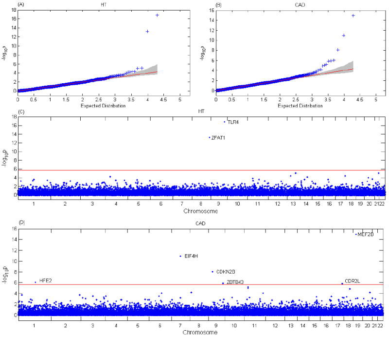
Association results of HT and CAD in the WTCCC data. (A) Q-Q plot of −log₁₀(P value) for the association test between HT and genes. The shaded region is the 95% confidence band. (B) Q-Q plot of −log₁₀(P value) for the association test between CAD and genes. (C) Genome-wide −log₁₀(P value) according to the chromosomal positions of genes in the association test for HT. The red horizontal line indicates a P value of 2.02×10^-6. Two genes with −log₁₀(P value) above the red line are identified. (D) Genome-wide −log₁₀(P value) according to the chromosomal positions of genes in the association test for CAD. The red horizontal line indicates a P value of 2.09×10^-6. Six genes with −log₁₀(P value) above the red line are identified.

Table 2.

Genes showing association evidence in the WTCCC HT and CAD samples in the stage 2 association test.

Genes	Chromosome	Cumulative risk haplotype frequency		Fisher exact test P-value	Are all SNPs good?
		Cases	Controls
Hypertension
TLR4	9q32-33	0.056	0.0188	1.76×10-16	No
ZFAT1	8q23-24	0.0384	0.0116	4.92×10-13	Yes
CAD
MEF2B	19p12	0.0372	0.0095	1.04×10-15	No
EIF4H	7q11.23	0.0120	0.0005	1.15×10-11	Yes
CDKN2B	9p21	0.2832	0.2247	8.75×10-9	No
HFE2	1q21	0.0065	0.0003	8.37×10-7	Yes
ZBTB43	9q33-34	0.0274	0.0119	1.29×10-6	Yes
CDR2L	17q25.1	0.0052	0.0	1.57×10-6	No

Because our two-stage analysis is dependent on how well the co-classification is performed at stage 1, which is dependent on the sample that is selected for stage 1, we then randomly selected 300 cases at stage 1 keeping the rest of the samples for the stage 2 analysis. We repeated this process 5,000 times and examined the percentages of each of the 5 genes (ZFAT1 for hypertension; EIF4H, CDKN2B, HFE2 and ZBTB43 for CAD) reaching genome-wide significance. We further compared with all the genes in the genome. Figure 7 presents the distribution of the number of times that a gene can reach the genome-wide significance level for all the genes among the 5,000 replications. The 5 genes ZFAT1, EIF4H, CDKN2B, HFE2 and ZBTB43, for which this occurred 58.9%, 88.2%, 38.9%, 21.9%, and 47.7% of the time, respectively, clearly stand out from the rest of the genes. In addition, we also observed the gene MACROD2 (17.8%) for HT and the gene LDHA (10.5%) for CAD that were missed before.

Figure 7.

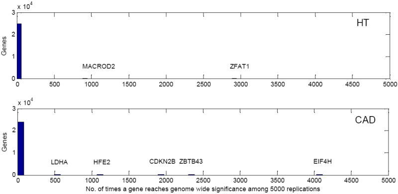
The distributions of the number of times a gene can reach the genome-wide significance level for all the genes across the genome among 1000 replications. Top: HT; bottom: CAD

Our simulation analysis also indicated that the power of our method is dependent on the cumulative risk haplotype frequency, which can affect the sample size to choose at stage 1. We used 300 cases at stage 1 on assuming the cumulative risk haplotype frequency is low. We then selected 500 cases at stage 1 and the rest of the samples for stage 2 and redid the analysis. We repeated this process 5,000 times and examined the percentage of times the 5 genes reached genome-wide significance. The results are consistent with those obtained when 300 cases were used at stage 1.

Finally, we examined the rare risk haplotypes for the 5 genes by comparing the rare risk haplotype frequencies between cases and controls using all the samples. Table 3 lists the risk haplotypes and their corresponding frequencies in all the cases and controls, as well as the Fisher exact p-values. The genes ZFAT1, CDKN2B and ZBTB43, but not EIF4H and HFE2, each includes more than three risk haplotypes.

Table 3.

Risk haplotypes and their corresponding frequencies in cases and controls for WTCCC HT and CAD data

Gene	Chr	Start SNP	End SNP	Haplotype	Freq in cases	Freq in controls	Fisher’s exact test p-value
HT
ZFAT1	8	rs6988616	rs11778878	001000101111100101111101100100	0.001281	0.000173	4.21×10-2
				001100100110110001000001101100	0.002049	0.000345	1.28×10-2
				001110101011100001010111111010	0.011527	0	1.40×10-18
				100100000101110011000001100100	0.004611	0.001553	4.94×10-3
				111010101011100001010111111010	0.012295	0	8.95×10-20
CAD
CDKN2B	9	rs3217986	rs10965245	000000010000000010101111100000	0.011942	0.005956	1.27×10-3
				100000010000000010101111100010	0.223780	0.189074	1.77×10-5
				100000010000000010101111100011	0.015576	0.007658	1.55×10-4
				101001101100111010101111100010	0.045691	0.037270	2.40×10-2
				101111010000000010101111100010	0.011423	0.007488	2.45×10-2
EIF4H	7	rs150880	rs17146094	0100	0.011942	0.000511	1.13×10-15
HFE2	1	rs12091564	rs10218795	00	0.006490	0.000511	6.54×10-8
ZBTB43	9	rs10987465	rs7038622	01001101100101	0.006750	0.000851	5.15×10-7
				01001111110001	0.003894	0.000511	1.86×10-4
				01101111110001	0.003894	0.000340	4.90×10-5

Discussion

We have proposed a two-stage method to detect association due to multiple rare variants in association studies. It should be noted that our method is based on detecting risk haplotypes rather than ungenotyped rare risk alleles, although we hypothesize the rare risk alleles fall on risk haplotypes. Using both simulations and real data, we demonstrated that the proposed two-stage method has reasonable power to reach a genome-wide significance level at a sample size comparable to that usually used for a whole genome association study design to detect common disease variants. However, the proposed method has no power in the case of a recessive mode of inheritance. For a recessive disease, it is much more difficult to observe any enrichment of risk alleles among cases compared to controls. To perform the two-stage analysis, the dataset is divided into two parts; one part is used for co-classifying rare risk haplotypes and the other is for association testing. We have also proposed two designs for the co-classifying stage: the unrelated-case and affected sibpair designs. We demonstrated that the affected sibpair design has better power to co-classify rare risk haplotypes than the unrelated-case design when the genotyping cost is the same. This is due to the risk haplotype frequencies being more enriched in affected sibpairs than in affected cases, as demonstrated in Figure 2. The power of co-classifying rare risk haplotypes decreases when the cumulative risk haplotype frequency increases. Our simulations showed that the power of the association test depends on both the relative sample sizes at stages 1 and 2 and the cumulative risk haplotype frequency. The higher the cumulative risk haplotype frequency, the larger the sample size we would use at stage 1. The reason for this is that we would then co-classify more risk haplotypes at stage 1; therefore, we will still have good power in the association test at stage 2 even though the sample size is relatively small because we have used more of the total sample at stage 1. We observed that 300-400 cases or 150-200 sibpairs, together with 1000 controls, at stage 1 can perform well when the cumulative risk haplotype frequency is relatively low. In practice, we can choose different sample sizes at stages 1 and 2 and compare whether the results at different sample sizes are similar. If in a particular gene the results are substantially different, we would examine whether the cumulative risk haplotype frequency is high or low.

For illustration, our simulation model assumed all rare risk haplotypes share a common relative risk, which is not the case in practice. However, our analysis does not need to make this assumption. It is possible that we can improve the proposed method by a weighted method in the stage 2 analysis, with the weights estimated from stage 1. For example, the weights can be the odds ratios of rare haplotypes estimated at stage 1. However, the performance of such a weighted method should be further studied in simulations.

Our simulations indicate that single SNP analysis does not have power when multiple rare risk variants contribute to a phenotype, even when a linkage signal can be detected. This may explain why many current GWAS have failed to detect variants in regions where linkage evidence had been reported in previous studies.

Our method is designed for application to data where mostly common SNPs are genotyped, such as in current GWAS, although the method can also be applied to resequencing data. Unlike the method of Li and Leal [Li and Leal 2008], who propose to collapse rare variants when all the rare variants in a dataset have been genotyped, our method co-classifies rare haplotypes by assuming that rare risk variants distribute on different haplotypes. Therefore in our method it is not necessary for the rare variants to have been genotyped. Since haplotype phase is usually unknown in practice, statistical methods[Browning and Browning 2007; Scheet and Stephens 2006; Stephens, et al. 2001] should be used to infer the phase. Our simulations indeed suggest power can suffer when haplotype phase is unknown, although the type I error remains reasonable. However, we observed that the loss of power is not substantial, even when we only used the most likely haplotypes inferred by PHASE. We also noticed that the loss of power is less for the affected sibpair design than for the unrelated-case design, suggesting that using family data to infer haplotype phase can be an advantage in detecting rare genetic variants, even though we used it only at the first stage.

Our proposed method is computationally much less intensive than the method recently proposed by Guo and Lin [Guo and Lin 2008], which applies a dimension-reduction method based on a generalized linear model with a regularization approach (rGLM) used in data mining and statistical learning. Since the asymptotic distribution of the method’s test statistic is unknown, a permutation procedure has to be applied. In GWAS, over a million permutations must be performed in order to accurately evaluate the p-value at the genome-wide significance level. Thus rGLM is infeasible in GWAS because of the tremendous computational burden. Rather than classifying risk haplotypes, rGLM weeds out the haplotypes that are not associated with the phenotype. Furthermore, when the number of risk haplotypes is large, the number of degree of freedom remains large, potentially reducing the power.

There was no gene reported to be associated with HT, and only one gene (CDKN2B) with CAD, in the original WTCCC report [2007]. We thus hypothesized that some genes might be associated with HT or CAD due to multiple rare variants and were therefore unlikely to be detected by single SNP association analysis. We applied our method to the WTCCC HT and CAD data and detected one and four novel genes significantly associated with HT and CAD, respectively. Although the association evidence between CDKN2B and CAD had been already established, because of being due to common variants, this gene was also identified in our analysis. However, we also noticed that genotyping errors due to bad SNP calling can result in false positive signals. For example, among the 8 genes detected in the initial analysis, 3 of them were due to the bad calling of individual SNPs. It is also possible for false positives to be introduced when the missing SNP genotyping rates are different between cases and controls. We compared the missing rates for the SNPs in these 5 genes and did not observe any significant difference, indicating that the significant findings are not due to different SNP missing rates between cases and controls.

Except for CDKN2B, which has been reported to be associated with CAD, the remaining 4 genes are novel. This is not surprising, given the rarity of the variants associated with these traits. However, we might expect some linkage evidence for these genes in family studies. In the linkage analysis of large pedigree data from South Italy, genome-wide significant linkage evidence to essential hypertension was reported on chromosome 8q22-23 [Ciullo, et al. 2006], where the ZFAT1 gene is located. We did not find any linkage evidence reported in previous studies for the 4 CAD genes, which may be attributed to the low power of linkage analysis.

However, we caution that the findings of the 5 genes for HT and CAD should be further replicated in independent studies. It could be a great challenge to replicate association evidence due to multiple rare variants, even within the same locus, particularly in different populations. The reason for this is that different populations very likely have different rare variants affecting the same phenotypic variation.

Although our two-stage method is computationally simple and has good power to detect rare genetic variants, it has several limitations. First, dividing samples into two parts is not optimal. Nevertheless, the cumulative risk haplotype frequency is increased, leading to more power in the association test for a set of risk haplotypes. Ideally, it would be most efficient if all the samples could be used for both co-classification and the association test. For example, we could calculate the p-values for every haplotype and then combine the evidence of a subset of haplotypes that reach nominal significance. However, the distribution of combined correlated p-values is unknown and the p-value might be best obtained by a permutation test. The reason for doing this is that the haplotypes are correlated (because of following a multinomial distribution) and many haplotypes are rare, and so a test based on an asymptotic distribution is not reliable. Furthermore, the distribution of the test statistic is different in different genes, making it difficult to compare the test statistic values across different genes. For genome-wide association studies, we need to conduct over a million permutations in order to obtain a reliable small p-value. Therefore, a one-stage method may not be computationally feasible. Our proposed method can thus be very useful in analyzing data from GWAS. Second, our proposed method is sensitive to genotype errors and requires extreme caution in its use. However, this is always a problem for methods to detect rare variants. If the genotype errors or genotyping missing is random, the type I error is not inflated for the proposed method. One of our future studies will assess how serious the effect of different nonrandom genotype error rates can be. Third, when analyzing the data from GWAS, the method requires breaking the genome into many chromosome segments. There are alternative ways for doing this, including haplotype block based methods. If a chromosome segment includes many rare variants, the power of the proposed method can be made better by analyzing the haplotypes in that segment, rather than in a haplotype block. In addition, haplotype blocks cannot capture well the variation due to rare variants. Thus, a gene-based analysis strategy can be better than haplotype block based methods, as we demonstrated in the application of our method to the WTCCC HT and CAD data. However, when multiple rare variants fall in a block with strong LD, a haplotype block based method can be better than a gene-based method.

In conclusion, we developed a two-stage method for detecting rare variants. This method can be straightforwardly extended to resequencing data when such data are available. Although our method is based on the assumption that multiple rare variants contribute to complex diseases, it can also detect genetic variants under the CD-CV assumption.

Appendix A

Rare risk haplotypes are enriched among cases

The frequency of a rare susceptible haplotype H_i among cases is

$$\begin{array}{l}P(H_i\mid \mathit{affected})=P(H_i{H}_i\mid \mathit{affected})+0.5\sum _{j\ne i}P(H_i{H}_j\mid \mathit{affected})\\ =\frac{P(\mathit{affected}\mid H_i{H}_i)P(H_i{H}_i)+0.5\sum _{j\ne i,j<=k}P(\mathit{affected}\mid H_i{H}_j)P(H_i{H}_j)+0.5P(\mathit{affected}\mid H_i{H}_{k+1})P(H_i{H}_{k+1})}{P(\mathit{affected})}\\ =\frac{f_2{h}_i+f_2\sum _{j\ne i,j<=k}{h}_j+h_{k+1}{f}_1}{P(\mathit{affected})}{h}_i\end{array}$$

1. Multiplicative: f₂ = λf₀, $f_1=\sqrt{\lambda }{f}_0$, we have

   $$\begin{array}{l}P(H_i\mid \mathit{affected})=\frac{\lambda p_i^2+\lambda p_i(p-p_i)+\sqrt{\lambda }{p}_i(1-p)}{p^2\lambda +2p(1-p)\sqrt{\lambda }+{(1-p)}^2}\\ =\frac{\sqrt{\lambda }}{\sqrt{\lambda }p+1-p}{p}_i.\end{array}$$
2. Dominant: f₂ = f₁ = λ f₀, we have

   $$P(H_i\mid \mathit{affected})=\frac{\lambda }{\lambda -{(1-p)}^2(\lambda -1)}{p}_i.$$
3. Recessive, f₂ = λ f₀, f₁ = f₀, we have

   $$P(H_i\mid \mathit{affected})=\frac{p(\lambda -1)+1}{p^2(\lambda -1)+1}{p}_i.$$

Rare risk haplotypes are enriched among affected sibpairs

Using the same notation as in the text and let s₁ and s₂ be two sibs of a sibpair, where s_i = 1 if the i-th sib is affected and 0 if not affected. Let I be the number of haplotypes shared identical by descent (IBD) by a sibpair. We have

$$P(H_i\mid s_1=s_2=1)=\frac{P(H_i,s_1=s_2=1)}{P(s_1=s_2=1)}.$$

Letting g₁, g₂ be the genotypes of two sibs and f_g the penetrance of genotype g, we have

$$P(s_1=s_2=1)=\sum _{I=0}^2\sum _{g_1,g_2}P(I,g_1,g_2,s_1=s_2=1)$$

$$\sum _{I=0}^2\sum _{g_1,g_2}P(s_1=s_2=1\mid g_1,g_2)P(g_1,g_2\mid I)P(I)=\sum _{I=0}^2\sum _{g_1,g_2}{f}_{g_1}{f}_{g_2}P(g_1,g_2\mid I)P(I).$$ (1)

Assume all the susceptible haplotypes have the same effect, that is, assume f_HiHj = f₂ if i <= k, j <= k, f_HiHj = f₁ if i ≤ k, j = k + 1, or i = k + 1, j ≤ k and H_HiHj = f₀ if i = j = k + 1, where k is the number of rare risk haplotypes. We then have Equation (1)

$$\begin{array}{l}=\sum _{I=0}^2\sum _{i=1}^{k+1}\sum _{j=1}^{k+1}\sum _{l=1}^{k+1}\sum _{m=1}^{k+1}{f}_{H_i{H}_j}{f}_{H_l{H}_m}P(H_i{H}_j,H_l{H}_m\mid I)P(I)\\ =\frac{1}{4}\sum _{i=1}^{k+1}\sum _{j=1}^{k+1}\sum _{l=1}^{k+1}\sum _{m=1}^{k+1}{f}_{H_i{H}_j}{f}_{H_l{H}_m}P(H_i)P(H_j)P(H_l)P(H_m)\\ +\frac{1}{2}\sum _{i=1}^{k+1}\sum _{j=1}^{k+1}\sum _{l=1}^{k+1}{f}_{H_i{H}_j}{f}_{H_j{H}_l}P(H_i)P(H_j)P(H_l)+\frac{1}{4}\sum _{i=1}^{k+1}\sum _{j=1}^{k+1}{f}_{H_i{H}_j}{f}_{H_i{H}_j}P(H_i)P(H_j)\\ =\frac{1}{4}{[f_2{p}^2+2f_{1}p(1-p)+f_0{(1-p)}^2]}^2\\ +\frac{1}{2}[f_2^2{p}^3+2f_1{f}_2{p}^2(1-p)+f_1^2{p}^2(1-p)+2f_0{f}_{1}p{(1-p)}^2+f_1^{2}p{(1-p)}^2+f_0^2{(1-p)}^3]\\ +\frac{1}{4}[f_2^2{p}^2+2f_1^{2}p(1-p)+f_0^2{(1-p)}^2].\end{array}$$

Similarly, when H_i is a risk allele, or i < k + 1, we have

$$\begin{array}{l}P(H_i,s_1=s_2=1)\\ =\sum _{I=0}^2\sum _{g_1,g_2}P(I,g_1,g_2,H_i,s_1=s_2=1),\\ =\sum _{I=0}^2\sum _{g_1,g_2}P(s_1=s_2=1\mid g_1,g_2)P(H_i\mid g_1,g_2)P(g_1,g_2\mid I)P(I)\\ =\sum _{I=0}^2\sum _{g_1,g_2}{f}_{g_1}{f}_{g_2}P(H_i\mid g_1,g_2)P(g_1,g_2\mid I)P(I)\\ =\frac{1}{4}\sum _{j,l,m=1}^{k+1}{f}_{H_i{H}_j}{f}_{H_l{H}_m}P(H_i)P(H_j)P(H_l)P(H_m)+\frac{1}{2}\sum _{j,l=1}^{k+1}{f}_{H_i{H}_j}{f}_{H_j{H}_l}P(H_i)P(H_j)P(H_l)+\frac{1}{4}\sum _{j=1}^{k+1}{f}_{H_i{H}_j}^{2}P(H_i)P(H_j)\\ =\frac{1}{4}{h}_i[f_2^2{p}^3+3f_1{f}_2{p}^2(1-p)+f_1{f}_0{(1-p)}^3+2f_1^{2}p{(1-p)}^2+f_2{f}_{0}p{(1-p)}^2]\\ +\frac{1}{2}{h}_i[f_2^2{p}^2+f_1{f}_{2}p(1-p)+f_1^{2}p(1-p)+f_0{f}_1{(1-p)}^2]+\frac{1}{4}{h}_i[f_2^{2}p+f_1^2(1-p)].\end{array}$$

1. Multiplicative: f₂ = λ f₀, $f_1=\sqrt{\lambda }{f}_0$, we have

   $$P(H_i\mid s_1=s_2=1)=\frac{\sqrt{\lambda }[{(\sqrt{\lambda }-1)}^3{p}^3+(2\sqrt{\lambda }+5){(\sqrt{\lambda }-1)}^2{p}^2+(\sqrt{\lambda }-1)(\lambda +3\sqrt{\lambda }+7)p+\sqrt{\lambda }+3]}{[{(\sqrt{\lambda }p+1-p)}^2+\lambda p+1-p^2]}{h}_i.$$

   The factor before h_i reflects the enrichment of the rare haplotype shared by affected sibpairs.

2. Dominant: f₂ = f₁ =λ f₀, we have

   $$P(H_i\mid s_1=s_2=1)=\frac{\frac{1}{4}\lambda [3p(p-2)(1-\lambda )+3+\lambda ]}{\frac{1}{4}{[\lambda p(2-p)+{(1-p)}^2]}^2+\frac{1}{2}[{\lambda }^2{p}^2(3-2p)+\lambda (2+\lambda )p{(1-p)}^2+{(1-p)}^3]+\frac{1}{4}[{\lambda }^{2}p(2-p)+{(1-p)}^2]}{h}_i.$$
3. Recessive, f₂ = λ f₀, f₁ = f₀, we have

   $$P(H_i\mid s_1=s_2=1)=\frac{1+\frac{1}{4}{(\lambda -1)}^2{p}^3+\frac{1}{4}(2\lambda +1)(\lambda -1)p^2+\frac{1}{4}(\lambda +4)(\lambda -1)p}{\frac{1}{4}{[\lambda p^2-p^2+1]}^2+\frac{1}{2}[1+{(\lambda -1)}^2{p}^3+2(\lambda -1)p^2)]+\frac{1}{4}[{\lambda }^2{p}^2-p^2+1]}{h}_i.$$

References

- The International HapMap Project. Nature. 2003;426(6968):789–96. doi: 10.1038/nature02168. [DOI] [PubMed] [Google Scholar]
- A haplotype map of the human genome. Nature. 2005;437(7063):1299–320. doi: 10.1038/nature04226. [DOI] [PMC free article] [PubMed] [Google Scholar]
- Genome-wide association study of 14,000 cases of seven common diseases and 3,000 shared controls. Nature. 2007;447(7145):661–78. doi: 10.1038/nature05911. [DOI] [PMC free article] [PubMed] [Google Scholar]
- Abecasis GR, Cherny SS, Cookson WO, Cardon LR. Merlin--rapid analysis of dense genetic maps using sparse gene flow trees. Nat Genet. 2002;30(1):97–101. doi: 10.1038/ng786. [DOI] [PubMed] [Google Scholar]
- Bhangale TR, Rieder MJ, Nickerson DA. Estimating coverage and power for genetic association studies using near-complete variation data. Nat Genet. 2008;40(7):841–3. doi: 10.1038/ng.180. [DOI] [PubMed] [Google Scholar]
- Bodmer W, Bonilla C. Common and rare variants in multifactorial susceptibility to common diseases. Nat Genet. 2008;40(6):695–701. doi: 10.1038/ng.f.136. [DOI] [PMC free article] [PubMed] [Google Scholar]
- Browning SR, Browning BL. Rapid and accurate haplotype phasing and missing-data inference for whole-genome association studies by use of localized haplotype clustering. Am J Hum Genet. 2007;81(5):1084–97. doi: 10.1086/521987. [DOI] [PMC free article] [PubMed] [Google Scholar]
- Chakravarti A. Population genetics--making sense out of sequence. Nat Genet. 1999;21(1 Suppl):56–60. doi: 10.1038/4482. [DOI] [PubMed] [Google Scholar]
- Ciullo M, Bellenguez C, Colonna V, Nutile T, Calabria A, Pacente R, Iovino G, Trimarco B, Bourgain C, Persico MG. New susceptibility locus for hypertension on chromosome 8q by efficient pedigree-breaking in an Italian isolate. Hum Mol Genet. 2006;15(10):1735–43. doi: 10.1093/hmg/ddl097. [DOI] [PubMed] [Google Scholar]
- Cohen J, Pertsemlidis A, Kotowski IK, Graham R, Garcia CK, Hobbs HH. Low LDL cholesterol in individuals of African descent resulting from frequent nonsense mutations in PCSK9. Nat Genet. 2005;37(2):161–5. doi: 10.1038/ng1509. [DOI] [PubMed] [Google Scholar]
- Cohen JC, Boerwinkle E, Mosley TH, Jr, Hobbs HH. Sequence variations in PCSK9, low LDL, and protection against coronary heart disease. N Engl J Med. 2006a;354(12):1264–72. doi: 10.1056/NEJMoa054013. [DOI] [PubMed] [Google Scholar]
- Cohen JC, Kiss RS, Pertsemlidis A, Marcel YL, McPherson R, Hobbs HH. Multiple rare alleles contribute to low plasma levels of HDL cholesterol. Science. 2004;305(5685):869–72. doi: 10.1126/science.1099870. [DOI] [PubMed] [Google Scholar]
- Cohen JC, Pertsemlidis A, Fahmi S, Esmail S, Vega GL, Grundy SM, Hobbs HH. Multiple rare variants in NPC1L1 associated with reduced sterol absorption and plasma low-density lipoprotein levels. Proc Natl Acad Sci U S A. 2006b;103(6):1810–5. doi: 10.1073/pnas.0508483103. [DOI] [PMC free article] [PubMed] [Google Scholar]
- Corder EH, Saunders AM, Strittmatter WJ, Schmechel DE, Gaskell PC, Small GW, Roses AD, Haines JL, Pericak-Vance MA. Gene dose of apolipoprotein E type 4 allele and the risk of Alzheimer’s disease in late onset families. Science. 1993;261(5123):921–3. doi: 10.1126/science.8346443. [DOI] [PubMed] [Google Scholar]
- Frazer KA, Ballinger DG, Cox DR, Hinds DA, Stuve LL, Gibbs RA, Belmont JW, Boudreau A, Hardenbol P, Leal SM, et al. A second generation human haplotype map of over 3.1 million SNPs. Nature. 2007;449(7164):851–61. doi: 10.1038/nature06258. [DOI] [PMC free article] [PubMed] [Google Scholar]
- Frikke-Schmidt R, Nordestgaard BG, Jensen GB, Tybjaerg-Hansen A. Genetic variation in ABC transporter A1 contributes to HDL cholesterol in the general population. J Clin Invest. 2004;114(9):1343–53. doi: 10.1172/JCI20361. [DOI] [PMC free article] [PubMed] [Google Scholar]
- Fullerton SM, Clark AG, Weiss KM, Nickerson DA, Taylor SL, Stengard JH, Salomaa V, Vartiainen E, Perola M, Boerwinkle E, et al. Apolipoprotein E variation at the sequence haplotype level: implications for the origin and maintenance of a major human polymorphism. Am J Hum Genet. 2000;67(4):881–900. doi: 10.1086/303070. [DOI] [PMC free article] [PubMed] [Google Scholar]
- Gabriel SB, Schaffner SF, Nguyen H, Moore JM, Roy J, Blumenstiel B, Higgins J, DeFelice M, Lochner A, Faggart M, et al. The structure of haplotype blocks in the human genome. Science. 2002;296(5576):2225–9. doi: 10.1126/science.1069424. [DOI] [PubMed] [Google Scholar]
- Gudbjartsson DF, Walters GB, Thorleifsson G, Stefansson H, Halldorsson BV, Zusmanovich P, Sulem P, Thorlacius S, Gylfason A, Steinberg S, et al. Many sequence variants affecting diversity of adult human height. Nat Genet. 2008;40(5):609–15. doi: 10.1038/ng.122. [DOI] [PubMed] [Google Scholar]
- Guo W, Lin S. Generalized linear modeling with regularization for detecting common disease rare haplotype association. Genet Epidemiol. 2008 doi: 10.1002/gepi.20382. [DOI] [PMC free article] [PubMed] [Google Scholar]
- Iyengar SK, Elston RC. The genetic basis of complex traits: rare variants or “common gene, common disease”? Methods Mol Biol. 2007;376:71–84. doi: 10.1007/978-1-59745-389-9_6. [DOI] [PubMed] [Google Scholar]
- Ji W, Foo JN, O’Roak BJ, Zhao H, Larson MG, Simon DB, Newton-Cheh C, State MW, Levy D, Lifton RP. Rare independent mutations in renal salt handling genes contribute to blood pressure variation. Nat Genet. 2008;40(5):592–9. doi: 10.1038/ng.118. [DOI] [PMC free article] [PubMed] [Google Scholar]
- Kissebah AH, Sonnenberg GE, Myklebust J, Goldstein M, Broman K, James RG, Marks JA, Krakower GR, Jacob HJ, Weber J, et al. Quantitative trait loci on chromosomes 3 and 17 influence phenotypes of the metabolic syndrome. Proc Natl Acad Sci U S A. 2000;97(26):14478–83. doi: 10.1073/pnas.97.26.14478. [DOI] [PMC free article] [PubMed] [Google Scholar]
- Kotowski IK, Pertsemlidis A, Luke A, Cooper RS, Vega GL, Cohen JC, Hobbs HH. A spectrum of PCSK9 alleles contributes to plasma levels of low-density lipoprotein cholesterol. Am J Hum Genet. 2006;78(3):410–22. doi: 10.1086/500615. [DOI] [PMC free article] [PubMed] [Google Scholar]
- Lander ES. The new genomics: global views of biology. Science. 1996;274(5287):536–9. doi: 10.1126/science.274.5287.536. [DOI] [PubMed] [Google Scholar]
- Lettre G, Jackson AU, Gieger C, Schumacher FR, Berndt SI, Sanna S, Eyheramendy S, Voight BF, Butler JL, Guiducci C, et al. Identification of ten loci associated with height highlights new biological pathways in human growth. Nat Genet. 2008;40(5):584–91. doi: 10.1038/ng.125. [DOI] [PMC free article] [PubMed] [Google Scholar]
- Li B, Leal SM. Methods for detecting associations with rare variants for common diseases: application to analysis of sequence data. Am J Hum Genet. 2008;83(3):311–21. doi: 10.1016/j.ajhg.2008.06.024. [DOI] [PMC free article] [PubMed] [Google Scholar]
- Luke A, Wu X, Zhu X, Kan D, Su Y, Cooper R. Linkage for BMI at 3q27 region confirmed in an African-American population. Diabetes. 2003;52(5):1284–7. doi: 10.2337/diabetes.52.5.1284. [DOI] [PubMed] [Google Scholar]
- Marchini J, Cardon LR, Phillips MS, Donnelly P. The effects of human population structure on large genetic association studies. Nat Genet. 2004;36(5):512–7. doi: 10.1038/ng1337. [DOI] [PubMed] [Google Scholar]
- McCarthy MI, Abecasis GR, Cardon LR, Goldstein DB, Little J, Ioannidis JP, Hirschhorn JN. Genome-wide association studies for complex traits: consensus, uncertainty and challenges. Nat Rev Genet. 2008;9(5):356–69. doi: 10.1038/nrg2344. [DOI] [PubMed] [Google Scholar]
- McPherson R, Pertsemlidis A, Kavaslar N, Stewart A, Roberts R, Cox DR, Hinds DA, Pennacchio LA, Tybjaerg-Hansen A, Folsom AR, et al. A common allele on chromosome 9 associated with coronary heart disease. Science. 2007;316(5830):1488–91. doi: 10.1126/science.1142447. [DOI] [PMC free article] [PubMed] [Google Scholar]
- Nyholt DR. A simple correction for multiple testing for single-nucleotide polymorphisms in linkage disequilibrium with each other. Am J Hum Genet. 2004;74(4):765–9. doi: 10.1086/383251. [DOI] [PMC free article] [PubMed] [Google Scholar]
- Perola M, Sammalisto S, Hiekkalinna T, Martin NG, Visscher PM, Montgomery GW, Benyamin B, Harris JR, Boomsma D, Willemsen G, et al. Combined genome scans for body stature in 6,602 European twins: evidence for common Caucasian loci. PLoS Genet. 2007;3(6):e97. doi: 10.1371/journal.pgen.0030097. [DOI] [PMC free article] [PubMed] [Google Scholar]
- Plenge RM, Cotsapas C, Davies L, Price AL, de Bakker PI, Maller J, Pe’er I, Burtt NP, Blumenstiel B, DeFelice M, et al. Two independent alleles at 6q23 associated with risk of rheumatoid arthritis. Nat Genet. 2007;39(12):1477–82. doi: 10.1038/ng.2007.27. [DOI] [PMC free article] [PubMed] [Google Scholar]
- Pritchard JK. Are rare variants responsible for susceptibility to complex diseases? Am J Hum Genet. 2001;69(1):124–37. doi: 10.1086/321272. [DOI] [PMC free article] [PubMed] [Google Scholar]
- Reich DE, Lander ES. On the allelic spectrum of human disease. Trends Genet. 2001;17(9):502–10. doi: 10.1016/s0168-9525(01)02410-6. [DOI] [PubMed] [Google Scholar]
- Risch N, Merikangas K. The future of genetic studies of complex human diseases. Science. 1996;273(5281):1516–7. doi: 10.1126/science.273.5281.1516. [DOI] [PubMed] [Google Scholar]
- Risch NJ. Searching for genetic determinants in the new millennium. Nature. 2000;405(6788):847–56. doi: 10.1038/35015718. [DOI] [PubMed] [Google Scholar]
- Romeo S, Pennacchio LA, Fu Y, Boerwinkle E, Tybjaerg-Hansen A, Hobbs HH, Cohen JC. Population-based resequencing of ANGPTL4 uncovers variations that reduce triglycerides and increase HDL. Nat Genet. 2007;39(4):513–6. doi: 10.1038/ng1984. [DOI] [PMC free article] [PubMed] [Google Scholar]
- Samani NJ, Erdmann J, Hall AS, Hengstenberg C, Mangino M, Mayer B, Dixon RJ, Meitinger T, Braund P, Wichmann HE, et al. Genomewide association analysis of coronary artery disease. N Engl J Med. 2007;357(5):443–53. doi: 10.1056/NEJMoa072366. [DOI] [PMC free article] [PubMed] [Google Scholar]
- Saxena R, Voight BF, Lyssenko V, Burtt NP, de Bakker PI, Chen H, Roix JJ, Kathiresan S, Hirschhorn JN, Daly MJ, et al. Genome-wide association analysis identifies loci for type 2 diabetes and triglyceride levels. Science. 2007;316(5829):1331–6. doi: 10.1126/science.1142358. [DOI] [PubMed] [Google Scholar]
- Scheet P, Stephens M. A fast and flexible statistical model for large-scale population genotype data: applications to inferring missing genotypes and haplotypic phase. Am J Hum Genet. 2006;78(4):629–44. doi: 10.1086/502802. [DOI] [PMC free article] [PubMed] [Google Scholar]
- Stephens M, Smith NJ, Donnelly P. A new statistical method for haplotype reconstruction from population data. Am J Hum Genet. 2001;68(4):978–89. doi: 10.1086/319501. [DOI] [PMC free article] [PubMed] [Google Scholar]
- Stratton MR, Rahman N. The emerging landscape of breast cancer susceptibility. Nat Genet. 2008;40(1):17–22. doi: 10.1038/ng.2007.53. [DOI] [PubMed] [Google Scholar]
- Thomson W, Barton A, Ke X, Eyre S, Hinks A, Bowes J, Donn R, Symmons D, Hider S, Bruce IN, et al. Rheumatoid arthritis association at 6q23. Nat Genet. 2007;39(12):1431–3. doi: 10.1038/ng.2007.32. [DOI] [PMC free article] [PubMed] [Google Scholar]
- Visscher PM. Sizing up human height variation. Nat Genet. 2008;40(5):489–90. doi: 10.1038/ng0508-489. [DOI] [PubMed] [Google Scholar]
- Walsh T, King MC. Ten genes for inherited breast cancer. Cancer Cell. 2007;11(2):103–5. doi: 10.1016/j.ccr.2007.01.010. [DOI] [PubMed] [Google Scholar]
- Wang K, Li M, Bucan M. Pathway-Based Approaches for Analysis of Genomewide Association Studies. Am J Hum Genet. 2007;81(6) doi: 10.1086/522374. [DOI] [PMC free article] [PubMed] [Google Scholar]
- Weedon MN, Lango H, Lindgren CM, Wallace C, Evans DM, Mangino M, Freathy RM, Perry JR, Stevens S, Hall AS, et al. Genome-wide association analysis identifies 20 loci that influence adult height. Nat Genet. 2008;40(5):575–83. doi: 10.1038/ng.121. [DOI] [PMC free article] [PubMed] [Google Scholar]
- Weiss KM, Terwilliger JD. How many diseases does it take to map a gene with SNPs? Nat Genet. 2000;26(2):151–7. doi: 10.1038/79866. [DOI] [PubMed] [Google Scholar]
- Zeggini E, Weedon MN, Lindgren CM, Frayling TM, Elliott KS, Lango H, Timpson NJ, Perry JR, Rayner NW, Freathy RM, et al. Replication of genome-wide association signals in UK samples reveals risk loci for type 2 diabetes. Science. 2007;316(5829):1336–41. doi: 10.1126/science.1142364. [DOI] [PMC free article] [PubMed] [Google Scholar]
- Zhu X, Bouzekri N, Southam L, Cooper RS, Adeyemo A, McKenzie CA, Luke A, Chen G, Elston RC, Ward R. Linkage and association analysis of angiotensin I-converting enzyme (ACE)-gene polymorphisms with ACE concentration and blood pressure. Am J Hum Genet. 2001;68(5):1139–48. doi: 10.1086/320104. [DOI] [PMC free article] [PubMed] [Google Scholar]
- Zhu X, Cooper RS, Luke A, Chen G, Wu X, Kan D, Chakravarti A, Weder A. A genome-wide scan for obesity in African-Americans. Diabetes. 2002;51(2):541–4. doi: 10.2337/diabetes.51.2.541. [DOI] [PubMed] [Google Scholar]
- Zhu X, Fejerman L, Luke A, Adeyemo A, Cooper RS. Haplotypes produced from rare variants in the promoter and coding regions of angiotensinogen contribute to variation in angiotensinogen levels. Hum Mol Genet. 2005;14(5):639–43. doi: 10.1093/hmg/ddi060. [DOI] [PubMed] [Google Scholar]
Associated Data
This section collects any data citations, data availability statements, or supplementary materials included in this article.